Comments on the nature of the bonding in oxygenated dinuclear copper enzyme models

Abstract

The nature of the bonding in model complexes of di-copper metalloenzymes has been analyzed by means of the electronic localization function (ELF) and by the quantum theory of atoms in molecules (QTAIM). The constrained space orbital variations (CSOV) approach has also been used. Density functional theory (DFT) and CASSCF calculations have been carried out on several models of tyrosinase such as the sole ${\text{Cu}}_2{\text{O}}_2^{2+}$ central core, the ${\text{Cu}}_2{\text{O}}_{\text{2}}{({\text{NH}}_{\text{3}})}_6^{2+}$ complex and the ${\text{Cu}}_2{\text{O}}_{\text{2}}{(\text{Imidazol})}_6^{2+}$ complex. The influence on the central Cu₂O₂ moiety of both levels of calculation and ligand environment have been discussed. The distinct bonding modes have been characterized for the two major known structures: [Cu₂(μ–η²: η²–O₂)]²⁺ and [Cu₂(μ–O₂)]²⁺. Particular attention has been given to the analysis of the O–O and Cu–O bonds and the nature of the bonding modes has also been analyzed in terms of mesomeric structures. The ELF topological approach shows a significant conservation of the topology between the DFT and CASSCF approaches. Particularly, three-center Cu–O–Cu bonds are observed when the ligands are attached to the central core. At the DFT level, the importance of self interaction effects are emphasized. Although, the DFT approach does not appear to be suitable for the computation of the electronic structure of the isolated Cu₂O₂ central core, competitive self interaction mechanisms lead to an imperfect but acceptable model when using imidazol ligands. Our results confirm to a certain extent the observations of [M.F. Rode, H.J. Werner, Theoretical Chemistry Accounts 4–5 (2005) 247.] who found a qualitative agreement between B3LYP and localized MRCI calculations when dealing with the Cu₂O₂ central core with six ammonia ligands.

1. Introduction

Dinuclear copper complexes are widely spread structures which have been conserved through evolution, being present in microorganisms as well as in plants and mammals. Due to their capabilities, like molecular oxygen transport (hemocyanin) or oxidation (tyrosinase), they have been subject to many theoretical [1–8] and experimental [9–10] investigations. Theoretically, their complicated electronic structures are particularly interesting due to the possibility of an antiferromagnetic coupling related to the open-shell singlet nature of the central metallic core. In fact, two principal arrangements (Fig. 1) are observed for Cu₂O₂ depending on the existence of an O–O bond. The first structure is [Cu₂ (μ–η²: η²–O₂)]²⁺ (structure A) which is associated with an O–O bond. The second [Cu₂(μ–O₂)]²⁺ (structure B), is characterized by an absence of O–O bond and by a significantly shorter Cu–Cu distance. It is generally acknowledged that structure A is associated to a peroxide dianion (O₂)²⁻ fragment bonded to two Cu(II) cations. On the contrary, the formal oxidation states of structure B atoms are Cu(III) and (O²⁻)₂. Previous theoretical studies [3–7,11] have shown the importance of the electronic correlation effects in the treatment of such molecules. Particularly, the necessity of taking account of both dynamic and non-dynamic parts of the correlation has been emphasized by Flock and Pierloot [3b], the CASPT2 approach appearing as the only method robust enough to capture successfully the correct spin states in the presence of these unusual compensations of correlation effects. Unfortunately, this limits considerably the study of such systems because of the computational time requirement of the CASPT2 approach. So, in order to build realistic model of such enzymes and to study their chemistry, it is necessary to introduce more approximations. For that reason, the broken symmetry density functional theory (DFT) approach appears to be a natural choice of methodology enabling the use of pseudo-spectral and density fitting approaches. Nevertheless, the applicability of DFT for such system has been extensively discussed [4b] since popular functionals encounter severe problems to describe correctly the electronic structure. These difficulties appear not only linked to the monodeterminental nature of the DFT which can be artificially extended by using an unrestricted broken symmetry approach in order to mimic the right electronic structure. In fact, the uncontrolled self interaction error arising in usual GGA functionals has been shown to be a key phenomenon when dealing with transition metals, acting directly on spin density values and enhancing charge transfer interactions.

Fig. 1.

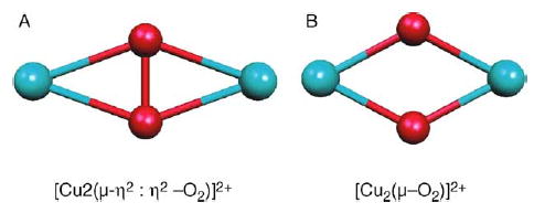
The two principal arrangements of the [Cu₂O₂]²⁺complex.

On the other hand, a recent study by Rode and Werner [11a] suggests that the CASPT2 approach strongly over-corrects the correlation effects, an MRCI approach using localized orbitals predicting results in qualitative agreement with B3LYP for such systems. These results have been since partially confirmed by Cramer et al. [11b] who also emphasized the CASPT2 deficiencies as well as the inaccuracy of the Couple Cluster approach for such open-shell low spin state systems.

In light of this new information, the goal of this paper is to come back to Density Functional Theory in order to estimate if its use could be acceptable for these systems, keeping in mind that accurate self interaction free density functionals are still under development. To do so, several tools for the bonding analysis have been used: the original electronic localization function (ELF) [12,13], the quantum theory of atoms in molecules [14] (QTAIM) and the constrained space orbital variations (CSOV) intermolecular energy decomposition scheme [15a–c].

Our approach is the following: since there is a competition between two electronic correlation effects (and since no CASPT2 or MRCI relaxed electronic densities are available), we will study them separately, the analysed densities being obtained using two approaches: DFT, including some dynamic correlations effects and multireferential CASSCF.

For that purpose, we chose to follow step by step the construction of a model of oxygenated di-copper enzyme. Electronic structures and geometries of three models of the enzymes will be considered and discussed, starting with the minimal [Cu₂O₂)]²⁺central moiety. In order to estimate ligand effects on [Cu₂O₂)]²⁺, two kind of complexes have been optimized. The first is the model chosen for previous [3b], CASPT2 [3b] and MRCI [11b] studies and involves simple NH₃ ligands to represent the nitrogen ligand environment of di-copper enzyme active sites. The second involves more realistic imidazol (Imh) ligands [8,11b], imidazol being closer to the side chain of the histidine residue occurring in hemocyanin and tyrosinase.

We will particularly discuss the influence of the self interaction on the bonding nature of the Cu–O and O–O bonds as well as some correlations between geometric parameters and bonding properties in the presence (or in the absence) of ligands.

2. Computational methods

All density calculations requested for the ELF and QTAIM analysis have been performed using GAUSSIAN 2003 [16] software and the DZVP2 basis set [17] (with diffuse functions on oxygens).

Broken symmetry geometry optimizations have been realized at the unrestricted B3LYP [18,19] and PBE0 [20] functionals levels whereas the closed-shell structures have been optimized at the restricted level. Geometry optimizations have also been performed at the CASSCF level. Our choice of a limited active space follows Eisenstein et al. [6] and is dictated by the need of optimized geometries in order to perform direct comparisons with the DFT results. The active space is made of 6 molecular orbital including dioxygen’s σ(10_ag), σ*(11_ag), the two π*(8b_1u, 2b_1g) orbitals plus the odd (5b_2u) and even (4b_3g) combinations of the copper d_xyz (and d_xz in the case of the parallel arrangement). These latter orbitals are particularly interesting since they have been shown to be at the origin of a Cu→O charge transfer [6]. The wave functions have been analyzed using the TopMod [21] package, and the graphical interpretation has been realized with Molekel [22]. For the CASSCF calculations the QTAIM charges have been obtained from the natural orbitals. The CSOV calculations have been performed using a modified version of HONDO 95.3 software [15b,23].

2.1. Topological analysis

In a topological analysis, a partitioning of the molecular space is achieved by the theory of dynamical systems. This partitioning gives a set of basins localized around the attractors (maxima) of the vector field of a scalar function. In the QTAIM [14] theory this scalar function is the electron density and the basins (Ω) are associated with each of the atoms in the molecule. Atomic properties such as the atomic population ( $\overline{N}$[Ω]) can then be calculated by integration over the basin defining an atom.

The topological analysis of the ELF function [24] has been extensively used for bonding analysis [25–33]. Indeed, ELF is interpretable in term of an excess of kinetic energy due to the Pauli repulsion [34]. Moreover, the relationship of the ELF function to the pair functions has been demonstrated [35]. In addition, the function is easily calculable and is bounded in the [0–1] interval. Such basins are classified as: core basins surrounding nuclei (if Z>2) and valence basins. The basins are characterized by their synaptic order. The core basin is denoted C(X), where X stands for a nucleus and is usually representative of electrons not involved in the chemical bonding, namely non-valence and internal-shell electrons known as such by chemists. The valence basins are distinguished according to the number of core basins with which they share a common boundary (synaptic order). A valence basin V(X) is monosynaptic and corresponds to lone-pair or non-bonding regions. A V(X, Y) basin is disynaptic: it bounds the core of two nuclei X and Y and, thus, corresponds to a bonding region between X and Y. It was shown that the basin distributions closely match to the VSEPR model [36,37]. The basin populations $\overline{N}$ are calculated by integrating the electron density in the basin volume. It is convenient to define the net charge transfer [25] (δq) from an atom A towards a fragment as $\delta q=Z(A)-\overline{N}[\text{C}(A)]-\overline{N}[\text{V}(A)].$ The integrated spin density 〈Sz〉 [38] can be also calculated for the open-shell singlet systems. The closure relation of the basin population operators enables a statistical analysis of the population to be made through the definitions of the variance [38] and the covariance matrix elements [39]. The variance of the basin population is interpreted as the population uncertainty, i.e. a measurement of the fluctuation for a given basin with all the other basins, while the values of the covariance matrix elements are a measure of the correlation between the populations of two given basins. This approach allows to describe the electronic structure of each system (A or B) in terms of superposition of the mesomeric structures [39]. For example, the electronic structure of the structure A can be described by a balance between three mesomeric structures:

$$\begin{array}{l}{\omega }_1:{[{\text{Cu}}_{\text{2}}^{\text{I}}(\mu -{\eta }^2:{\eta }^2-{\text{O}}_{\text{2}})]}^{2+};\\ {\omega }_2:{[{\text{Cu}}^{\text{I}}{\text{Cu}}^{\text{II}}{(\mu -{\eta }^2:{\eta }^2-{\text{O}}_{\text{2}})}^{-}]}^{2+};\\ {\omega }_3:{[{\text{Cu}}_{\text{2}}^{\text{II}}{(\mu -{\eta }^2:{\eta }^2-{\text{O}}_{\text{2}})}^{2-}]}^{2+}\end{array}$$

The first structure ω₁ corresponds to an interaction between two Cu^I atoms and the O₂ closed-shell singlet molecule $({}^{\text{1}}\sum {}_{\text{g}}^{+}).$ ω₁ is associated to a formal charge transfer δq = 1. The second structure, ω₂, involves a Cu^I interacting with a Cu^II and a doublet super oxide (O₂)⁻(²π_gi). ω₂ corresponds to δq = 1.50. The last structure ω₃ corresponds to an interaction between two Cu^II cations and a peroxide closed-shell singlet dianion (O₂)²⁻ $({}^{\text{1}}\sum {}_{\text{g}}^{+}).$ The ω₃ structure is consistent with δq = 2. The ω₁, ω₂ and ω₃ structures involve, respectively, three distinct oxides O₂ $({}^{\text{1}}\sum {}_{\text{g}}^{+}),{\text{O}}_2^{-}{(}^2{\mathrm{\Pi }}_{\text{gi}})$ and ${\text{O}}_2^{2-}({}^{\text{1}}\sum {}_{\text{g}}^{+}).$ At the B3LYP/DZVP2 level, the population analysis gives the following distribution:

$$\begin{array}{ccccc}& {\text{O}}_{\text{2}}& {\text{O}}_2^{-}& {\text{O}}_{\text{2}}^{\text{2}-}& \\ \overline{N}[\text{V}(\text{O})]& 2.56& 2.92& 3.29& \text{Oxygen lone pair}\text{.}\\ \overline{N}[\text{V}({\text{O}}_1,{\text{O}}_2)]& 1.64& 1.16& 0.68& {\text{O}}_{\text{1}}-{\text{O}}_{\text{2}}\text{ bond}\text{.}\end{array}$$

Consequently, the valence populations of each oxide provide the number of electrons assigned to the valence basins for each structure A. This assignment allows to build the following system:

$$\{\begin{array}{c}{\omega }_1+{\omega }_2+{\omega }_3=1\\ 2.56{\omega }_1+2.92{\omega }_2+3.29{\omega }_3=\overline{N}[\text{V(Cu},\hspace{0.17em}\text{O)}]\\ 1.64{\omega }_1+1.16{\omega }_2+0.68{\omega }_3=\overline{N}[{\text{V}(\text{O}}_{\text{1}},\hspace{0.17em}{\text{O}}_{\text{2}})]\end{array}$$ (1),(2)

The weights are determined in order to yield populations in good agreement with the reference calculations and reasonable values for the covariance matrix elements. For example, this approach provides the respective weights ω₁ = 0.55, ω₂ = 0.31 and ω₃ = 0.14 for the open-shell singlet structure obtained with the PBE0 functional (A-PBE0_OSSC). Thus, the covariance matrix of this model can be built as follow:

$$\begin{array}{c}\overline{N}[\text{V(Cu},\text{\hspace{0.17em}O)}]=\text{2}\text{.77}\\ \overline{N}[{\text{V(O}}_{\text{1}},{\text{O}}_{\text{2}}\text{)}]=\text{1}\text{.36}\end{array}\hspace{0.17em}\to \text{Cov}=\left(\begin{array}{cc}0.10& -0.09\\ -0.09& 0.11\end{array}\right)$$

where for example, Cov(1,2) = Cov(2,1) = 2.56 × 1.64× ω₁ + 2.92 × 1.16 × ω₂ + 3.29 × 0.68 × ω₃ − $\overline{N}[\text{V(Cu},\text{\hspace{0.17em}O)}]\times \hspace{0.17em}\overline{N}[{\text{V(O}}_{\text{1}},{\text{O}}_{\text{2}}\text{)}]$ ≈ −0.09. Thus, the model appears in reasonable agreement with the reference calculations:

$$\begin{array}{c}\overline{N}[\text{V(Cu},\text{\hspace{0.17em}O)}]=\text{2}\text{.77}\\ \overline{N}[{\text{V(O}}_{\text{1}},{\text{O}}_{\text{2}}\text{)}]=\text{1}\text{.32}\end{array}\hspace{0.17em}\to \text{Cov}=\left(\begin{array}{cc}0.42& -0.14\\ -0.14& 0.35\end{array}\right)$$

Moreover, the additional spin contraint 〈Sz〉 = 0 for the closed-shell systems allows to simplify the calculations since the weight of ω₂ must be zero. In this case, only the balance ω₁↔ω₃ will be considered.

2.2. The constrained space orbital approach (CSOV)

At available theory levels (HF, MCSCF and DFT), CSOV decomposes the total intermolecular interaction energy as:

$$\begin{array}{l}{E}_{\text{tot}}=E_{\text{FC}}+E_{\text{pol}}+E_{\text{ct}}\\ =E_{\text{coulomb}}+E_{\text{exc}-\text{rep}}+E_{\text{polA}}+E_{\text{polB}}+E_{\text{ctA}\to \text{B}}+E_{\text{ctB}\to \text{A}}\end{array}$$

The ‘frozen core’ energy (E_FC), which is the sum of the electrostatic (E_coulomb) and exchange/Pauli repulsion (E_exc/rep). The CSOV values for E_coulomb and E_exc/rep are identical to Morokuma’s Es and Eexch/rep if computed at the same level of theory. The electrostatic energy corresponds to the classic Coulomb interaction of the electron distributions of the isolated monomers, kept ‘frozen’, that is, not perturbed, into the A–B complex arrangement [5b]. E_coulomb includes a short range term related to the penetration of the charge distributions, and a long-range multipolar component which is usually approximated by a multipolar expansion. The exchange-repulsion term, which results from the Pauli Exclusion Principle, is calculated as the difference between E_FC and E_coulomb. The other, ‘non-frozen’ terms, are the polarization (E_pol) and charge transfer (E_ct) contributions, which depend on the variation of the molecular orbital and their eigenvalues due to the intermolecular interaction. Here, it is important to point out that both polarization and charge-transfer contributions are computed using antisymmetrized wave functions to avoid problems in complexes involving strong polarizing fields.

3. Results and discussions

All geometries of complexes have been fully optimized at both DFT and CASSCF levels.

Since previous studies [3b] (and references herein) have shown that the singlet state is more stable, no triplet calculations have been carried out. For these particular complexes, Pierloot and Flock [3b] have shown that the geometry B was favored by a large active space CASPT2 calculations in which both dynamic and non-dynamic correlation are taken into account.

Our calculations do not reflect both competitive effects because of the nature of the used methodologies but give separate informations on the different competitive effects: dynamic correlation for DFT and non-dynamic correlation for CASSCF.

For that reason, we observe a contradiction between the results obtained at both level of theory. All the optimized structures at the DFT level indicate to a global minimum corresponding to the structure A and the CASSCF predicts a B-type binding mode.

It is possible to obtain a B-type structure (OSSC) using a DFT broken symmetry approach. No restricted local minimum has been found but a single point restricted calculation at the OSSC geometry equilibrium was performed (see Table 1).

Table 1.

Energies of the ${\text{Cu}}_{\text{2}}{\text{O}}_{\text{2}}^{\text{2}+}$ structures (A and B) at B3LYP/DZVP2, PBE0/DZVP2 or CASSCF/DZVP2 levels

A-structures	Energy (u.a)	B-structures	Energy (u.a)
(PBE0)OSSCa	−3429.2949
(B3LYP)csb	−3429.9952	(B3LYP)csb,c	−3429.9121
(B3LYP)OSSCa	−3430.0444	(B3LYP)OSSCa	−3429.9542
(CASSCF)	−3426.0124	(CASSCF)	−3426.0547
NH3-(B3LYP)c csb	−3769.9942	NH3 (B3LYP)csb	−3769.9671
NH3-(B3LYP)OSSCa	−3770.0062
NH3-(CASS)	−3763.7245	NH3(CASSCF)	−3763.7828
Imh-(B3LYP) csb	−4788.2497
Imh-(B3LYP) OSSCa	−4788.2673
Imh-(CASSCF)	−4775.7140

^aOpen-shell singlet structure.

^bClosed-shell singlet structure.

^cSingle point at open-shell minimum.

For the A-type binding mode, the open-shell singlet structure obtained with the B3LYP functional (B3LYP_OSCC) is more stable by 31 kcal/mol than the restricted solution. We can notice that the OSSC character is associated with a slightly larger O–O bond (1.287 vs. 1.430 Å). The open-shell singlet structure obtained with the PBE0 functional (PBE0_OSCC) has also been found, but we were unable to find a PBE0 restricted solution since the calculation systematically leads to a dissociated complex. Moreover, in all cases, shorter O–O distances are observed in DFT compared to CASSCF.

Comparative atomic QTAIM charges for both A-type and B-type structures are listed in Table 2. For each structure, the copper charge is larger than 1.10. The A-type is quite consistent with a low copper charge whereas the B-type shows a high copper charge. In all cases, the OSCC structures show a larger copper charge than the closed-shell structures. Moreover, the CASSCF calculations are always in favor of a greater cationic character of the copper atoms (Table 3).

Table 2.

Atomic charges (AIM) for the structures A and B arrangements

	dO–O (Å)	q(Cu)	q(O)
A-(B3LYP)cs	1.274	1.10	−0.10
A-(PBE0)OSSC	1.287	1.14	−0.14
A-(B3LYP)OSSC	1.308	1.16	−0.16
A-(CASSCF)	1.477	1.69	−0.69
A-NH3 (B3LYP)OSSC	1.430	1.07	−0.60
A-NH3 (CASSCF)	1.491	1.38	−0.77
A-Imh (B3LYP)OSSC	1.403	0.98	−0.42
A-Imh (CASSCF)	1.471	0.89	−0.38
B-(B3LYP)OSCC	2.478	1.30	−0.28
B-(CASSCF)	2.596	1.61	−0.60
B-NH3 (B3LYP)CS	2.227	1.08	−0.68
B-NH3 (CASSCF)	2.630	1.33	−0.73

q(Cu) = Z(Cu)− $\overline{N}$ [Ω(Cu)] and q(O) = Z(O)− $\overline{N}$[Ω(O)]. $\overline{N}$[Ω(Cu)] and $\overline{N}$[Ω(O)] are the atomic populations.

Table 3.

CSOV analysis for the imidazol and ammonia copper (I) complexes

Energy (kcal/mol)	Cu(I)–ImH	Cu(I)–NH3
EFrozen Core	−28.1	−28.9
Epol (ligand)	−28.0	−13.5
Epol (Cu)	−11.4	−9.8
ECharge tranfer (metal→ligand)	−7.0	−4.4
ECharge tranfer (ligand→metal)	−7.2	−8.2
Total interaction energy	−81.7	−64.8

Figs. 2 and 3 display the localization domains of the ELF function for A-type and B-type bonding modes, respectively. The structure A exhibits four bonding basins V(Cu, O) and one bonding basin V(O₁, O₂) whereas the structure B does not show any V(O₁, O₂) basin. However, the structure B displays two monosynaptic V(O) basins which are interpreted as oxygen lone pairs. For the structure A, the V(O₁, O₂) basin is quite consistent with the covalent character of the O–O bond (in agreement with the small O–O distance).

Fig. 2.

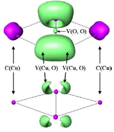
Localization domains of Cu₂(μ–η²: η² –O₂)²⁺ (A). Closed-shell singlet structure. Optimized B3LYP/DZVP2. The isosurfaces are ELF = 0.75 (top) and ELF = 0.88 (bottom).

Fig. 3.

Localization domains of the $\text{C}{\text{u}}_{\text{2}}\text{(}\mu -{\text{O}}_2^{2+})$ open-shell singlet structure (B). Optimized B3LYP/DZVP2. The isosurfaces are ELF = 0.75 (left) and ELF = 0.86 (right).

Table 4 gives the ELF population analysis for the two structures obtained with the B3LYP and PBE0 functionals. In order to specify the nature of the Cu–O interaction, we introduce the net electronic charge transfer quantity δq from the copper as Z(Cu)– $\overline{N}$[C(Cu)]. δq is a measurement of the electronic exchange from one Cu atom towards the remaining valence basins. Therefore, δq is related to the copper charge and its value is always positive from 1.16 to 1.61. However, the QTAIM analysis reveals that the substantial part of the population of the V(Cu, O) basin comes from the electron density localized on the oxygen atoms. Therefore, the Cu–O interaction can be described as a balance between the density donation from the oxygen and a small net electronic contribution Cu→O as indicated by δq.

Table 4.

ELF population analysis of structures A and B

Structures A
	[C(Cu)]		[V(Cu, O)]		[V(O1, O2)]	δq
	$\overline{N}$	〈Sz〉	$\overline{N}$	〈Sz〉	$\overline{N}$
(B3LYP)csa	27.84	–	2.77	–	1.36	1.16
(B3LYP)OSSCb	27.74	0.10	2.81	−0.05	1.27	1.26
(PBE0)OSSCb	27.77	0.08	2.77	−0.04	1.32	1.23
			$\overline{N}$[V(Cu1; O; Cu2)]
NH3(B3LYP)csa	27.53	–	3.06	–	0.66	1.47
NH3(B3LYP)OSSCb	27.26	0.09	3.22	−0.04	0.59	1.74
Imh(B3LYP)csa	27.54	–	3.07	–	0.56	1.46
Imh(B3LYP)OSSCb	27.52	0.02	3.04	−0.01	0.52	1.48

Structures B
	[C(Cu)]		[V(Cu, O)]		[V(O)]
	$\overline{N}$	〈Sz〉	$\overline{N}$	〈Sz〉	$\overline{N}$	〈Sz〉	δq
(B3LYP)OSSCb	27.39	0.24	1.79	−0.06	2.97	−0.12	1.61
NH3 (B3LYP)OSSC	27.52	0.01	3.04	−0.01	0.52	0.00	1.48

Population $\overline{N}$, integrated spin densities 〈S_z〉 and δq=Z(Cu)– $\overline{N}$[C(Cu)].

^aClosed-shell singlet structure.

^bOpen-shell singlet structure at DFT/DZVP2 level. The A-type structure displays two core basins C(Cu), four bonding basins V(Cu, O) and only one bonding basin V(O₁, O₂). The B-type structure displays two core basins C(Cu), four bonding basins V(Cu, O) and two V(O) corresponding to the lone pairs.

3.1. Structure Cu₂(μ–η²: η²–O₂)²⁺ (A-type)

Table 4 gives the ELF population analysis of A structures obtained with the B3LYP and PBE0 functionals. For the A-type structure, the population of V(O₁, O₂) is close to 1.3 electrons and the spin integrated density 〈Sz〉 is almost fully localized in both C(Cu) and V(Cu, O) basins. This is an indicator of the good electronic pairing of the O–O bond since the spin integrated density of the V(O₁, O₂) appears negligible.

As shown in Fig. 4, a linear correlation can be found between the O–O distances and the δq values (r² = 0.99), the O–O interaction being directly linked to the density delocalization from Cu towards the dioxygen fragment. This point is particularly interesting because the O–O distance can be directly used to estimate the importance of the density delocalization. For example, Fig. 4 allows to simulate δq for the CASSCF case knowing the O–O distance value (1.477 Å). This approximation leads to δq = 1.80 which appears quite consistent with the QTAIM population $\overline{N}$[Ω(Cu)] = 1.69. Therefore, by extrapolation, it becomes possible to estimate the other populations of the simulated valence basins for the CASSCF case since the population of the V(O₁,O₂) basin can be also correlated to the O–O distance. This way, we obtain the following simulated populations:

Fig. 4.

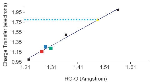
Charge transfer quantity (δq) as the O–O distance for the structures A obtained with the DFT calculations. Code color: red=B3LYP_closed-shell, blue=B3LYP_OSCC and green=PBE0_OSCC. The formal structures ω₁(δq=1.0), ω₂(δq=1.5) and ω₃(δq=2.0) are also displayed (black squares). The yellow dot is the simulated value for the CASSCF case. The line corresponds to the linear regression (r²=0.99). (For interpretation of the reference to colour in this legend, the reader is referred to the web version of this article.)

$$\begin{array}{l}\overline{N}[\text{C(Cu)}]=Z(\text{Cu})-\delta q=27.2;\\ \overline{N}[{\text{V(O}}_{\text{1}},{\text{O}}_{\text{2}})]=0.82\mathrm{\hspace{0.17em} }\text{and }\overline{N}[\text{V}(\text{Cu},\text{O})]=3.20\end{array}$$

We enclose to our study the three formal arrangements ω₁, ω₂, ω₃ which have an integer copper oxidation degree. ω₁ is associated to the Cu^I/Cu^I configuration, ω₂ to Cu^I/Cu^II mixing and ω₃ corresponds to the Cu^II/Cu^II configuration. In order to describe the binding mode, we propose to use a mesomeric occupation scheme (as previously explained in Section 2). Our purpose is not to discuss the value of the real charges in the ${\text{Cu}}_{\text{2}}{\text{O}}_{\text{2}}^{\text{2}+}$ systems but rather to show that the DFT or the CASSCF description may be related to the mesomeric scheme involving these three formal structures. As the DFT values can be directly computed, the application of the method to the CASSCF case is more sensitive. Indeed, we have only the simulated populations and several possible weight sets (ω₁, ω₂, ω₃) can be obtained. However, the QTAIM analysis predicts charges closer to +2 (see Table 2) compared to the one obtained at the DFT level. That way it is possible to remove the uncertainty as only one set shows a significant ω₃ weight. For both levels of theory, the typical distributions are:

$$\begin{array}{cccc}\text{B3LYP\hspace{0.17em}Closed\hspace{0.17em}}-\text{Shell Singlet}& {\omega }_{\text{1}}(72\%)& {\omega }_2(0\%)& {\omega }_3(28\%)\\ \text{PBE0\hspace{0.17em}Open\hspace{0.17em}}-\text{Shell Singlet}& {\omega }_1(55\%)& {\omega }_2(31\%)& {\omega }_3(14\%)\\ \text{B3LYP\hspace{0.17em}Open\hspace{0.17em}}-\text{Shell Singlet}& {\omega }_{\text{1}}(43\%)& {\omega }_2(39\%)& {\omega }_3(18\%)\\ \text{CASSCF}& {\omega }_{\text{1}}(6\%)& {\omega }_2(7\%)& {\omega }_3(87\%)\end{array}$$

The DFT open-shell electronic structures appear to be the consequence of a fine balance between the ω₁ and ω₂ configurations, the copper atoms being intermediate between a Cu^I and Cu^II. On the contrary, the CASSCF structure is essentially described by the ω₃ configuration leading to a better description of the antiferromagnetic coupling.

It is important to point out that in the case of an ELF topological analysis performed on CASSCF natural orbitals, the relations between the resulting CASSCF topological ‘domains’ and usual ELF ‘chemical’ basins remain unclear (due to the monodeterminantal nature of ELF). For that reason, the QTAIM analysis appears more suitable for a direct comparison of DFT and CASSCF atomic population. Nevertheless, it remains possible to perform a qualitative view at the CASSF level to compare the number and the nature (synaptic order) of the electronic domains to those obtained at the DFT level of theory. In the present case, the topological analysis found the same number of domains for both approaches.

3.2. Structure $C{u}_{\text{2}}\text{(}\mu -O_2^{2+})$(B-type)

Table 4 gives the ELF population analysis for the B-type B3LYP_OSCC structures. In contrast to structure A, structure B is characterized by a large δq close to 1.60. The absence of O–O coupling is due to the oxygen lone pairs described by two V(O) basins. On the other hand, the population of V(Cu, O) is smaller than in A because of a concentration of the δq delocalization into the V(Cu, O) and V(O) basins. The integrated spin density is mainly localized in the three basins C(Cu), V(Cu, O) and V(O). Structure B shows a partial antiferromagnetic coupling between the Cu centers with 〈S_z〉= 0.24 (in comparison to a perfect antiferromagnetic structure where 〈S_z〉=0.50). This result is in good agreement with the conclusions of the previous studies [3,5,6].

The geometrical parameters show the relevance of CASSCF calculations in describing an antiferromagnetic coupling where the non-dynamical correlation is very large. Consequently, according to the previous logical way, the large copper charge calculated for the CASSCF case (q(Cu)=1.61) is rather consistent with a large open-shell character. We can also describe B in the DFT case by a mixing of the two following structures according to the ELF population analysis: ω₄: [Cu^ICu^II ${(\mu -\text{O)}}_2^{-}$]²⁺ and ω₅:[ ${\text{Cu}}_2^{\text{II}}$(μ − O⁻)₂]²⁺. The ω₄ configuration describes a partial copper–oxygen coupling in correlation with δq=1.5. The ω₅ structure corresponds to a perfect antiferromagnetic configuration. The calculated weights in the DFT case provide a distribution of 78% for ω₄ and 22% for ω₅. This result is in agreement with the idea of a partial coupling. While, CASSCF should prefer the ω₅ configuration in agreement with the QTAIM charges (see Table 2), weight values cannot be calculated for the CASSCF case. Nevertheless, it is still possible to use a simple inspection of the wavefunction to corroborate this hypothesis, the diagonal elements of the final one electron density matrix reflecting an occupation close to 1 for the molecular orbitals localized on both copper and oxygen atoms.

3.3. Lone pairs and self interaction

Our results show that the interconversion between the two binding modes is driven by the redistribution of the electrons describing the lone pairs of the dioxygen. Obviously, this redistribution cannot be well represented at the DFT level since the initial electronic structures are plagued with a spin delocalization on the oxygen atoms. The mechanism in place, which is mainly due to a self interaction problem, can be analysed. First, it is important to note that B3LYP generally overestimates the value of the molecular polarizability 〈α〉 (〈α〉=1/3(α_xx+α_yy+α_zz)). Here, our results show a significant increase (17%) of the molecular polarizability of a singlet ((¹Σ)) dioxygen molecule in DFT (〈α〉_B3LYP=6.9933 au³) compared to post Hartree–Fock methodology (〈α〉_MP2= 5.8163 au³). In the presence of a strong electric field generated by the copper cation, the O₂ molecule is overpolarized, especially in the lone pair area which is bearing most of the total molecular polarizability of the molecule. Indeed, the direct consequence of this self interaction effect in DFT was not only an enhancement of the intermolecular polarization energy but also of the charge transfer interaction energy [15c]. This leads to the incorrect spin delocalization. In fact, the unrestricted wave functions needed to mimic the multi-reference Cu₂O₂ problem are not eigenfunctions of the total spin operator S² (they are only eigenfunctions of S_z). That way, in the case of an open-shell electronic structure (we have here an antiferromagnetic coupling) we have 〈S²〉^UKS>S(S+1) leading to an inevitable and uncontrolled spin delocalization [33]. The Cu₂O₂ appears like a worst case scenario for self interactions effects. Indeed, Zhang et al. pointed out [40] that larger self interaction effects could be observed in the case of fractional populations. Here, the intrinsic defects of the broken symmetry approach are multiplied by the interaction of very polarizable oxygen with the strong electric field generated by the metal cation.

It is also interesting to point out that a direct modification of the percentage of exact exchange [4b,c] in the functional is probably not a key for the treatment of such systems. Indeed, the results obtained with the PBE0 functional which embodies a different percentage of exact exchange than B3LYP are not really better than this latter, proposing only a slightly different electronic structure. Adding more exact exchange would certainly lead to a better control of the self interaction error but would also have a cost by limiting the treatment of dynamic correlation (the risk is to come back to a Hartree–Fock like behavior of the functional).

3.4. Ligands influence on [Cu₂O₂)]²⁺ central core

Table 2 gives the QTAIM charges while Table 4 gives the population analysis of [(Cu(L)₃)₂(μ–η²: η²–O₂)]²⁺ (denoted A–L) and [(Cu(L)₃)₂ (μ–O)₂]²⁺ (denoted B–L) complexes. The effects of the NH₃ molecule and the Imidazol (Imh) ligand on [Cu₂O₂)]²⁺ moiety have been analyzed in this section. The localization domains of A-NH₃ molecule are displayed on Fig. 5.

Fig. 5.

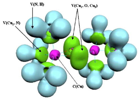
Localization domains (ELF=0.72) of the molecule A-NH₃. Optimized B3LYP/DZVP2 closed-shell singlet structure. Color code: magenta=core, green=valence polysynaptic, light blue=protonated valence disynaptic. (For interpretation of the reference to colour in this legend, the reader is referred to the web version of this article.)

The principal modification in A–L complexes is the presence of trisynaptic basins V(Cu₁, O, Cu₂) which are intrinsically associated with a weakening of the Cu–O bonding strength. Trisynaptic basins can be found above and below the Cu–O–Cu–O molecular plane whereas the V(Cu, O) basin of A-type lies in the molecular plane between Cu and O atoms.

3.4.1. Difference between NH₃ and imidazol ligands

The V(Cu₁, O, Cu₂) basin exists for both A-NH₃ and A-Imh structures obtained with the B3LYP functional. Nevertheless, the Imh influence on the central core Cu₂O₂ leads to a breaking of the C_2h symmetry, an O–O fragment lying above the molecular plane (butterfly effect). In addition, the copper charge increases as well as the δq quantity, which was about 1.26 for A-(B3LYP)_OSCC compared to 1.74 in the A-(B3LYP)NH_3OSCC. Therefore, the ligand effects on the di-copper central structure may be separated in two distinct influences. First, the Cu–N bond involves a density contribution of the copper. Second, the ligand induces a reorganization of the density in the central structure. In presence of ligands, the O–O interaction appears also weakened, being associated to a decrease of the V(O₁, O₂) basin population (compared to the sole central Cu₂O₂ moiety of A-type) and to a longer O–O distance (varying within the range 1.403 and 1.491 Å depending on the method -CASSCF giving always a longer bonding distance). On the contrary, the population of the V(Cu₁, O, Cu₂) basin is always higher than three electrons.

If in both cases (NH₃ and Imh), the disynaptic basins V(Cu, N) are consistent with a covalent character of the Cu–N bonds. It appears that the ligand effect can be illustrated by the population analysis on binary system Cu(L)⁺. Indeed, it is important to point out that the general picture of ‘N donor ligand’ has to be carefully examined when dealing with DFT calculation on metal cation complexes. The QTAIM analysis which uses an atomic basins partition captures this global effect and shows for both binary systems Cu–L (L=NH₃ or ImH) a population of the copper atomic basins of 28.27e in accordance with a net N donor effect. In fact, NH₃ ligands are generally seen as unable to receive a strong charge transfer from Cu( $\overline{N}$C(Cu)=28 electrons) because of their saturated valence shell leading to a limited back-donation.

Table 3 shows a CSOV analysis at the B3LYP level for the imidazol and ammonia copper (I) complexes. In fact, despite the observation of a relatively strong net donor effect (copper contributions to the Cu–N bonds), the metal→ligand charge transfer appears non-negligible at the B3LYP level, its value being close to half of the charge transfer (ligand→metal) contribution value. For the imidazol ligand which is expected to be a better electronic acceptor than NH_3, the CSOV calculation shows some significant differences.

First, the donation appears smaller than for NH₃ and is almost of the same magnitude as the backdonation leading to a weak donor effect only. Second, in the presence of an Imh ligand, the CSOV analysis shows a smaller participation of E_FC in the total stabilization than for NH₃. As the ratio E_FC/E_tot is a good indicator of the nature of the interaction [41], the Cu–N bond exhibits a significantly stronger covalent character in presence of an Imh ligand (polarization and charge transfer energies being dominant).

A partial intra-ligand delocalization appears linked to a more strongly polarized Imh ligand (E_pol (Imh) is about −28.0 kcal/mol) compared to NH₃ (E_pol (NH₃)=−13.5 kcal). This phenomenon can be also observed using the ELF approach, the position of the attractor related to the V(Cu–N) disynaptic basin being different for the two ligands. For the Imh ligand, the position of the V(Cu–N) basin attractor appears to be closer to the nitrogen (1.116 Å) than for NH₃. Here also, the strong polarization/charge transfer mechanism is another consequence of the self interaction effects and was observed previously on very similar Zn(II)-imidazol complex (Cu(I) and Zn(II) being isoelectronic) studied by CSOV [15c]. These artifacts have the same important consequences than the ones observed in presence of Zn(II): the interaction energies appear significantly larger in B3LYP than in MP₂.

3.5. Consequences of the ligand choice on the models

Ligand effects on the central Cu₂O₂ core can be observed when computing QTAIM charges (Table 2). Indeed, the values of the copper charges for A-NH₃ are consistent with the results obtained for the Cu₂O₂ isolated core A structure, showing significant differences between the DFT and CASSCF levels. In other words, the more electrostatic interaction of the ammonia ligands has fewer effects on the electronic configuration of Cu₂O₂ whereas the more covalent interactions of the Imh ligands are able to partially reorganize the electronic structure of the central core. That way a qualitative agreement is found between CASSCF and B3LYP QTAIM charges when Imh are present. The self interaction artifact generates a competitive electronic delocalization mechanism between O₂ and ImH (where traces of spin are found) which is not present in the NH3 case. Another possible explanation could be that the better agreement between DFT and CASSCF level indicates a possible decrease of the influence of non-dynamic correlation effects. Only more sophisticated CASSCF/CASPT2 or MRCI calculations would provide the final solution and the use of a greater active space (for a detailed analysis see the recent work of Cramer et al. [11b]) will be necessary to properly test this hypothesis. Here also, the study indicates that the complexes show an electronic structure compatible with a Cu^I/Cu^II model, the ELF copper population being close to 27.54 electrons and the participation of the copper in the bonding being limited (weak net CSOV charge transfer and very polarized ligand). Once again, a remarkable conservation of the topological qualitative view is observed between the DFT and CASSCF levels.

In contrast to the A-NH₃, the topological structure of B-NH₃ is very close to the one of the B-type. Indeed, two valence V(O) basins and disynaptic V(Cu,O) basins are observed. As for the A-NH₃ structure, the charge transfer δq increases.

4. Conclusion

Our results show that the two structures Cu₂(μ–η²: η²–O₂)²⁺ and ${\text{Cu}}_{\text{2}}{\text{(}\mu -\text{O)}}_{\text{2}}^{\text{2}+}$ are clearly distinguished by the ELF topological analysis. The A complex is characterized by a strong covalent character O–O and a small charge transfer Cu→O. In contrast, the B structure is described by two V(O) basins and a stronger charge transfer Cu→O. In agreement with previous studies, we have found an influence of the level of calculation. Indeed, the electronic structure of the B antiferromagnetic complex is well described at CASSCF level because its multideterminant nature imposes a treatment of non-dynamical correlation effects. For this kind of complex, the DFT approach appears definitely less accurate. Because of its single determinant nature, the broken symmetry method offers an access to a partial recovery of the antiferromagnetic coupling but it is plagued by the self interaction error leading to uncontrolled spin delocalization on the oxygen atoms. Despite these problems, some facts can be observed. For example, the positive charge transfer, correlated to the weights on mesomeric structures, implies a very different oxidation state of the copper atoms for the two structures. In contrast to the A binding mode, the B-type electronic structure shows a high copper oxidation degree according to a consistent antiferromagnetic coupling.

Moreover, the inter-conversion process from A to B complex is carried out by a decrease of the populations of the V(Cu, O) and V(O₁, O₂) (i.e.: the lone pairs) basins over the monosynaptic V(O) basin. This process appears very sensitive to the methodology, the oxygen lone pairs being subject to large self interaction errors at the DFT level. A theoretical study of such phenomenon should be, without doubt, reserved to advanced post Hartree–Fock methodologies even if important disagreements recently appear between them [3b,11a,b].

The A-L complexes, which are the most stable at the DFT level, show topological modifications compared to original Cu₂O₂ core electronic structure: a more complex three centers bond can be observed through the trisynaptic basin V(Cu₁, O, Cu₂). However, The NH₃ ligand can be distinguished from the Imidazol ligand by a weaker charge transfer Cu→O and by a less covalent interaction with the central metal core. The Imh ligand model presents a modification of the complex symmetry (butterfly effect). At the DFT level, the competitive self interaction effects between ImH and O₂ reduce the charge delocalization on the oxygen observed for the other complexes.

These results show that the consequences of the self interaction problem in DFT are probably more complex than usually admitted and can include competitive mechanisms. The choice of Imh as ligand leads to a model, providing a partial antiferromagnetic coupling. Obviously the model appears not to be perfect but involves a Cu^I/Cu^II oxidation state of the coppers and an (O₂)⁻ fragment which can be enough to study these particular enzymes since they appear to be consistent with some experimental functional di-copper protein models [42]. In all cases, an encouraging aspect is the conservation of the topological partition of the systems at the CASSCF and DFT levels. In other words, a qualitative agreement exists in all cases despite a spurious spin delocalization. Obviously, this problem appears more critical for a small model where the spin states are dominant. At the opposite when ligands are added, an electronic redistribution occurs and the importance of non-dynamical correlation effects appears to decrease. This point confirms the observation of Rode and Werner [11a] who found a qualitative agreement between a localized MRCI approach and a DFT B3LYP calculation, both confirming a more stable A-type binding mode in the presence of NH₃ ligands, characteristic of dominant dynamic correlation effects.

References

- 1.Ross PK, Solomon EI. J Am Chem Soc. 1991;113:3246. [Google Scholar]
- 2.Chen P, Solomon I. J Inorg Biochem. 2002;88:368. doi: 10.1016/s0162-0134(01)00349-x. [DOI] [PubMed] [Google Scholar]
- 3.Cramer CJ, Smith BA, Tolman WB. J Am Chem Soc. 1996;118:11283. (a) [Google Scholar]; Flock M, Pierloot K. J Phys Chem A. 1999;103:95. (b) [Google Scholar]
- 4.Lind T, Siegbahn PEM, Crabtree RH. J Phys Chem B. 1999;103:1193. (a) [Google Scholar]; Lind T, Siegbahn PEM. Faraday Discuss. 2003;124:289. doi: 10.1039/b211811b. (b) [DOI] [PubMed] [Google Scholar]; Lind T, Chen P, Root DE, Campochiaro C, Fujisawa K, Solomon EI. J Am Soc. 2003;125:466. doi: 10.1021/ja020969i. (c) [DOI] [PubMed] [Google Scholar]
- 5.Ruiz E, Alemany P, Alvarez S, Cano J. J Am Chem Soc. 1997;119:1297. (a) [Google Scholar]; Ruiz E, De Graaf C, Alemany P, Alvarez S. J Phys Chem A. 2002;106:4938. (b) [Google Scholar]
- 6.Eisenstein O, Getlicherman H, Giessner-Prettre C. J Maddaluno, Inorg Chem. 1997;36:3455. doi: 10.1021/ic9515766. [DOI] [PubMed] [Google Scholar]
- 7.Nikolov GS, Mikosh H, Baeur G. J Mol Struct. 2000;35:499. [Google Scholar]
- 8.Piquemal JP, Maddaluno J, Silvi B, Giessner-Prettre C. New J Chem. 2003;27:909. [Google Scholar]
- 9.Murthy N, Mahroof-Tahir M, Karlin KD. Inorg Chem. 2001;40:628. doi: 10.1021/ic000792y. (a) [DOI] [PubMed] [Google Scholar]; Santagostini L, Gullotti M, Monzani E, Casella L, Dillinger R, Tuczek F. Chem Eur J. 2000;6:519. doi: 10.1002/(sici)1521-3765(20000204)6:3<519::aid-chem519>3.0.co;2-i. (b) [DOI] [PubMed] [Google Scholar]; Kitajima N, Fujisawa K, Fujimoto C, Morooka Y, Hashimoto S, Kitagawa T, Toriumi K, Tatsumi K, Nakamura A. J Am Soc. 1992;114:1277. (c) [Google Scholar]; Itoh S, Kumei H, Taki M, Nagatomo S, Kitagawa T, Fukuzum S. J Am Chem Soc. 2001;123:6708. doi: 10.1021/ja015702i. (d) [DOI] [PubMed] [Google Scholar]; Klabunde T, Eicken C, Sacchetini JC, Krebs B. Nat Struct Biol. 1998;5:1084. doi: 10.1038/4193. (e) [DOI] [PubMed] [Google Scholar]; Gerdemann C, Eicken C, Krebs B. Acc Chem Res. 2002;35:183. doi: 10.1021/ar990019a. (f) [DOI] [PubMed] [Google Scholar]; Maddaluno JF, Faull KF. Experientia. 1998;44:885. doi: 10.1007/BF01941189. (g) [DOI] [PubMed] [Google Scholar]; Conrad JS, Dawso SR, Hubbard ER, Strothkamp KG. Biochemistry. 1994;33:5739. doi: 10.1021/bi00185a010. (h) [DOI] [PubMed] [Google Scholar]
- 10.Sanchez-Ferrer A, Rodriguez-Lopez JN, Garcia-Canovas F, Garcia-Carmona F. Biochim Biophys Acta. 1996;1:1247. doi: 10.1016/0167-4838(94)00204-t. [DOI] [PubMed] [Google Scholar]
- 11.Rode MF, Werner HJ. Theor Chem Acc. 2005;4–5:247. (a) [Google Scholar]; Cramer CJ, Wloch M, Piecuch P, Puzzarini C, Gagliardi L. J Phys Chem A. 2006;110:1991. doi: 10.1021/jp056791e. (b) [DOI] [PubMed] [Google Scholar]
- 12.Becke AD, Edgecombe KE. J Chem Phys. 1990;92:5397. [Google Scholar]
- 13.Kohout M, Savin A. Int J Quantum Chem. 1996;60:875. [Google Scholar]
- 14.Bader RFW. Oxford University Press; Oxford: 1990. Atoms in Molecules: A Quantum Theory. [Google Scholar]
- 15.Bagus PS, Hermann K, Bauschlisher CW., Jr J Chem Phys. 1984;4378:80. (a) [Google Scholar]; Bagus PS, Bagus PS, Illas F. J Chem Phys. 1992;463:96. (b) [Google Scholar]; Piquemal J-P, Marquez A, Parisel O, Giessner Prettre C. J Comp Chem. 2005;1052:26. doi: 10.1002/jcc.20242. (c) [DOI] [PubMed] [Google Scholar]
- 16.Frisch MJ, Trucks GW, Schlegel HB, Scuseria GE, Robb MA, Cheeseman JR, Montgomery JA, Jr, Vreven T, Kudin KN, Burant JC, Millam JM, Iyengar SS, Tomasi J, Barone V, Mennucci B, Cossi M, Scalmani G, Rega N, Petersson GA, Nakatsuji H, Hada M, Ehara M, Toyota K, Fukuda R, Hasegawa J, Ishida M, Nakajima T, Honda Y, Kitao O, Nakai H, Klene M, Li X, Knox JE, Hratchian HP, Cross JB, Adamo C, Jaramillo J, Gomperts R, Stratmann RE, Yazyev O, Austin AJ, Cammi R, Pomelli C, Ochterski JW, Ayala PY, Morokuma K, Voth GA, Salvador P, Dannenberg JJ, Zakrzewski VG, Dapprich S, Daniels AD, Strain MC, Farkas O, Malick DK, Rabuck AD, Raghavachari K, Foresman JB, Ortiz JV, Cui Q, Baboul AG, Clifford S, Cioslowski J, Stefanov BB, Liu G, Liashenko A, Piskorz P, Komaromi I, Martin RL, Fox DJ, Keith T, Al-Laham MA, Peng CY, Nanayakkara A, Challacombe M, Gill PMW, Johnson B, Chen W, Wong MW, Gonzalez C, Pople JA. Gaussian Inc.: Pittsburgh, PA; 2003. GAUSSIAN 03, Revision A.1. [Google Scholar]
- 17.Godbout N, Salahub DR, Andzelm J, Wimmer E. Can J Chem. 1992;70:560. [Google Scholar]
- 18.Becke AD. Phys Rev A. 1988;38:3098. doi: 10.1103/physreva.38.3098. [DOI] [PubMed] [Google Scholar]
- 19.Lee C, Yang W, Parr RG. Phys Rev B. 1988;37:785. [Google Scholar]
- 20.Adamo C, Barone V. J Chem Phys. 1999;110:6158. [Google Scholar]
- 21.Noury S, Krokidis X, Fuster F, Silvi B. Comput Chem. 1999;23:597. [Google Scholar]
- 22.Flukiner P, Luthi HP, Portman S, Weber J, Molekel . Switzerland: Swiss Center for Scientific Computing. 2002. [Google Scholar]
- 23.Dupuis M, Marquez A, Davidson ER. Indiana University; Bloomington, IN: 1995. HONDO 95.3, QCPE. [Google Scholar]
- 24.Silvi B, Savin A. Nature. 1994;371:683. [Google Scholar]
- 25.Pilme J, Alikhani E, Silvi B. J Phys Chem A. 2003;107:4506. [Google Scholar]
- 26.Silvi B, Pilmé J, Fuster F, Alikhani ME. What can tell topological approaches on the bonding in transition metal compounds. In: Russo N, Salahub DR, Witko M, editors. Metal–Ligand Interactions, ATO ASI SCIENCES SERIES: II: Mathematics, Physics and Chemistry. Kluwer; Dordrecht: 2003. p. 241. [Google Scholar]
- 27.Llusar R, Beltrán A, Andrés J, Noury S, Silvi B. J Comput Chem. 1999;20:1517. [Google Scholar]
- 28.Choukroun R, Donnadieu B, Zhao JS, Cassoux P, Lepetit C, Silvi B. Organometallics. 2000;19:1901. [Google Scholar]
- 29.Chesnut DB, Bartolotti LJ. Chesnut DB, Chesnut DB, Bartolott LJ. Chem Phys. J Chem Phys. 2000;2000;253257:1. 171. [Google Scholar]
- 30.Fressigné C, Maddaluno J, Marquez A, Giessner-Prettre C. J Org Chem. 2001;65:8899. doi: 10.1021/jo000648u. [DOI] [PubMed] [Google Scholar]
- 31.Noury S, Silvi B, Gillespie RG. Inorg Chem. 2002;41:2164. doi: 10.1021/ic011003v. [DOI] [PubMed] [Google Scholar]
- 32.Pilmé J, Silvi B B, Alikhani EA. J Phys Chem A. 2005;109:10028. doi: 10.1021/jp053170c. [DOI] [PubMed] [Google Scholar]
- 33.Chevreau H, De II, Moreira PR, Silvi B, Illas F. J Phys Chem A. 2001;105:3570. [Google Scholar]
- 34.Savin A, Nesper R, Wengert S, Fässler TF. Angew Chem Int Ed Engl. 1997;36:1809. [Google Scholar]
- 35.Silvi B. J Phys Chem A. 2003;107:3081. [Google Scholar]
- 36.Gillespie RJ, Popelier PLA. Oxford University Press; Oxford: 2001. Chemical Bonding and Molecular Geometry. [Google Scholar]
- 37.Gillespie RJ. Van Nostrand Reinhold; London: 1972. Molecular Geometry. [Google Scholar]
- 38.Savin A, Silvi B, Colonna F. Can J Chem. 1996;74:1088. [Google Scholar]
- 39.Silvi B. PCCP. 2004;2:256. [Google Scholar]
- 40.Zhang Y, Yang W. J Chem Phys. 1998;109:2604. [Google Scholar]
- 41.Gourlaouen C, Piquemal JP, Saue T, Parise O. J Comput Chem. 2006;27:142. doi: 10.1002/jcc.20329. [DOI] [PubMed] [Google Scholar]
- 42.Van Gastel M, Bubacco L, Groenen JJ, Vijgenboom E, Canters GW. FEBS Lett. 2000;474:228. doi: 10.1016/s0014-5793(00)01609-4. [DOI] [PubMed] [Google Scholar]