Residue-Level Prediction of DNA-Binding Sites and its Application on DNA-Binding Protein Predictions

Abstract

Protein-DNA interactions are crucial to many cellular activities such as expression-control and DNA-repair. These interactions between amino acids and nucleotides are highly specific and any aberrance at the binding site can render the interaction completely incompetent. In this study, we have three aims focusing on DNA-binding residues on the protein surface: develop an automated approach for fast and reliable recognition of DNA-binding sites; improving the prediction by distance-dependent refinement and use these predictions to identify DNA-binding proteins. We use a support vector machines (SVM)-based approach to harness the features of the DNA-binding residues to distinguish them from non-binding residues. Features used for distinction include the residue’s identity, charge, solvent accessibility, average potential, the secondary structure it is embedded in, neighboring residues, and location in a cationic patch. These features collected from 50 proteins are used to train SVM. Testing is then performed on another set of 37 proteins, much larger than any testing set used in previous studies. The testing set has no more than 20% sequence identity not only among its pairs, but also with the proteins in the training set, thus removing any undesired redundancy due to homology. This set also has proteins with an unseen DNA-binding structural class not present in the training set. With the above features, an accuracy of 66% with balanced sensitivity and specificity is achieved without relying on homology or evolutionary information. We then develop a postprocessing scheme to improve the prediction using the relative location of the predicted residues. A balanced success is then achieved with average sensitivity, specificity and accuracy pegged at 71.3%, 69.3% and 70.5%, respectively. Average net prediction is also around 70%. Finally, we show that the number of predicted DNA-binding residues can be used to differentiate DNA-binding proteins from non-DNA-binding proteins with an accuracy of 78%. Results presented here demonstrate that machine-learning can be applied to automated identification of DNA-binding residues and that the success rate can be ameliorated as more features are added. Such functional site prediction protocols can be useful in guiding consequent works such as site-directed mutagenesis and macromolecular docking.

1. Introduction

The interactions between protein and DNA control many paramount cellular processes, such as transcription, replication, DNA repair, recombination and other critical steps in cellular development [1]. Consequentially, these interactions have received proportionate interest from molecular biologists over the past three decades, and recently, from computational biologists [2,3]. Recent molecular and structural studies have augmented our comprehension of these specific interactions. Structure genomic projects are solving the structures of protein-DNA complexes at an alarming rate. As much as this inundation of information equips us with clues for finding patterns in these interactions, it also gives rise to the need for methods and tools that predict the DNA-binding function of a new protein and the binding sites on its molecular surface [3,4].

Methods for prediction of specific protein-DNA interaction sites can be categorized in two main classes: the prediction of the binding DNA sequence in the genome, and the prediction of binding site on the protein. The first category has been addressed profusely; specifically various tools/methods have been advanced [5], including the usage of consensus sequence [6], weight matrices [7], information content [8] and protein-DNA recognition patterns [9].

There have been fewer computational studies addressing the second problem. Experimental techniques towards the discovery of DNA-binding residues on protein surface include site-directed mutagenesis studies [10], where specific sites are mutated and their effect on DNA binding are studied. These experiments can be prohibitively labor-intensive in studying all possible mutations of the residues on the molecular surface. Automated recognition of binding residues can facilitate these experiments by narrowing down the potential sites to be studied. Identification of DNA-binding sites on a protein surface can also help in function annotation [11]. Therefore, a fast and reliable computational method to identify these sites would be very useful.

A few computational protocols have been developed for automated identification of DNA-binding residues based on the features derived from sequence and structure collectively and those from sequence alone. Among earliest attempts, Ahmad et al. developed neural networks using sequential features from a dataset of 62 proteins and achieved 40.6% sensitivity and 76.2% specificity with 3-fold cross validation that resembles holdout evaluation [12]. As these were sequence-based predictions all the residues including the interior ones were used for prediction. Using both sequential and structural information, specificity and sensitivity achieved was 40.3% and 81.8%, respectively [12]. They further integrated evolutionary profiles into the prediction and achieved higher performance with 68.2% and 66% sensitivity and specificity, respectively, with 6-fold cross-validation [13]. Using the same dataset and leaving residues from one protein out for testing in each iteration, Kuznetsov et al. applied Support Vector Machines for identification of DNA-binding sites on the basis of sequential/structural features with 71% accuracy and balanced values of sensitivity and specificity [14]. With the addition of profile of evolutionary conservation of sequence positions in the form of a Position Specific Scoring Matrix (PSSM), they achieved higher performance with 79.2% sensitivity and 85.4% specificity [14]. Yan et al. developed Naïve Bayes classifier for sequence-based prediction of DNA-binding residues registering 71% accuracy and added sequence entropy of the target residue as an additional input to achieve 78% accuracy [15] leaving residues from one protein (from a set of 171 proteins) for testing.

In this work, we accomplish three aims: we develop an SVM-based classifier for automated identification of DNA-binding residues, including the ones located on novel folds, with a high and balanced performance based on the features derived from both sequence and structure; develop a set of post-processing techniques to further improve the performance; and, demonstrate that prediction of DNA-binding residues can be used to identify DNA-binding proteins with high accuracy. SVM [16] is a powerful classification tool that has found various applications in bioinformatics, including fold recognition [17–19], gene expression analysis [20], homology detection [21] and identification of DNA-binding proteins [22] or membrane-binding proteins [23]. Here, we design the dataset and methods addressing some specific issues. First, to improve structure-based prediction we only use the surface residues (see definition under Methods) to form training/testing dataset. Second, we leave out a large dataset (residues from 37 proteins; larger than used in any previous similar study) for testing using holdout evaluation. Third, the dataset was divided into training and testing dataset in a way that testing set includes some proteins belonging to one of the structural classes or folds that are not present in training set. These eight major structural classes include helix-turn-helix, zinc-binding, leucine zipper, other alpha-helix, β-sheet, β-hairpin/ribbon, enzymes and others listed by Luscombe et al. [1]. This way our classifier was made to identify DNA-binding residues embedded in some novel structural folds. It should also be noted that using evolutionary information that relies on alignment with homologous sequences introduces conservation effects and may not work when the protein has no close homologs. We do not use any kind of conservation information for descriptors and our dataset has less than 20% pairwise sequence identity. We use an assemblage of descriptors to differentiate the binding residues from non-binding ones. These features include the identity of the residues, the charge of a residue, its location in a large cationic patch, the neighboring residue composition, the secondary structure it is buried in, its solvent accessibility and its average electrostatic potential. These properties are translated into feature vectors and put into SVM, which are then trained on the basis of these properties. Next, the model generated by the SVM classifier is tested to identify binding sites on a new set of proteins using holdout evaluation and show promising, balanced prediction power.

All the descriptors used above are the properties of a single residue; they do not include a collective reinforcement to boost the performance. After the above mentioned prediction, we develop a set of protocols to further advance the prediction of the binding sites using distance-dependent refinement of the initial classification. First we ‘enrich’ the classification by labeling those residues as positive that have a certain number of neighboring residues predicted to be binding. In another step of ‘trimming’, we label those residues as negative that are isolated from positively predicted residues. While the first step increases the number of true positives, the second one reduces the number of false positives. We show that these steps increase the prediction performance and make it more balanced in terms of sensitivity and specificity.

We further show that prediction of DNA-binding residues on protein surface can be effectively used to identify DNA-binding proteins. Using the above developed protocol, residues on the surface of DNA-binding and non-DNA-binding proteins are predicted. We find that number of residues predicted can be effectively used to differentiate DNA-binding proteins from non-DNA-binding and the distinction becomes clearer with the application of refinement steps mentioned above.

This paper is organized as follows. In method section, we describe the dataset used and the classification and validation methods employed. In results, we present the performances of our current protocol, and its improvement after post-processing. We then analyze the improvement in the prediction over the currently published protocols and discuss future research directions.

2. Materials and Methods

Dataset

For the present study, a set of 150 protein-DNA complexes of crystallographic resolution better than 3 Å was formed by the union of previous related studies [12,24–26]. This set was divided into two subsets: Set I consisting of randomly-selected 50 proteins which formed the training set and Set II of 96 proteins forming the testing set. Sequence identity was reduced to 20% within the testing set to remove redundancy due to homology (which distorts the results). Proteins in the test set with more than 20% identity with proteins belonging to the training set were also removed, resulting in a total of 37 proteins in the testing set. This set also included proteins from a structural class, namely the β–sheet; the training set did not have any protein belonging to this class. A complete list of the proteins used here is available at http://proteomics.bioengr.uic.edu/pro-dna.

Definition of a surface binding residue

Hydrogen atoms were added to all the structures using the publicly-available software package REDUCE [27]. DSSP [28] was then used to calculate the exposed surface area of all residues. A residue was classified as a “surface” residue if it had more than 40% of its total area exposed. Otherwise it was classified as “buried”. Furthermore, a surface residue was defined as “binding” if any of its heavy atoms was within a distance of 4.5 Å to any atom of the DNA.

Descriptor design

1) Net charge of a residue

Due to a negative ambience around the DNA, charge reciprocality of a residue may play an important role in its binding to the DNA. Therefore, the net charge of a residue was used as a feature for classification. A charge of +1 was ascribed to Arg and Lys and -1 to Asp and Glu. His was specified a charge of +0.5 and all other residues were taken as neutral.

2) Occurrence in a cationic patch

Presence of large regions of positive electrostatic patches has been shown to insinuate location of DNA-binding sites [24,29]. We located such cationic patches on the protein surface. Delphi (v4) [30,31] was used for all electrostatic calculations in this study. This tool solves the non-linear Poisson-Boltzmann using finite-difference methods to calculate the potential at specified points. Electrostatic potentials at the site of all the atoms in a protein were reported in the absence of the DNA. The CHARMM22 [32] force-field parameters were employed for assignment of partial charges to the atoms. Detailed description of the parameters used for the calculation can be found elsewhere [22]. We located the four largest cationic patches on the molecular surface. These patches were then sorted by their sizes and each residue was associated with the patch it was present in. A feature equal to 4 was assigned to a residue if it was present in the first largest patch, 3 if it was present in the second largest patch, so on, and 0 if it was not present in any of the first four patches.

3) Average Potential on a residue

We also used the average electrostatic potential on a residue as one of the descriptors. After calculating the potential at the site of every atom of a residue, it was assigned a potential equal to the average of the potentials on all its atoms.

4) Secondary structure

We appraised six secondary structures for any inclination towards any particular structural state and computed the relative frequency of amino acids in these states. These secondary structures included alpha helix, isolated beta-bridge, extended strand, 3-helix (3/10 helix), 5 helix (pi helix), hydrogen-bonded turn and bend [28]. DSSP was used to assign every residue to one of the six structural classes. We also calculated the binding propensity of a residue present in a particular structural state by dividing the number of binding residues present in that secondary structure by the total number of residues in the same structure.

5) Solvent Accessible Surface Area (ASA)

We calculated the relative ASA of every residue from DSSP in order to determine the correlation of ASA with a residue's propensity to bind.

6) Structural neighbors of the residue

Protein-DNA interactions originate from multiple interactions between the two sides and do not involve a single residue-base interaction [12]. For a specific locale on a protein to be in contact with the DNA, the compatibility of its neighborhood may also be significant. Therefore, the identities of neighbors in contact with each residue were also used as a descriptor comprising a 20 feature-long vector with each element equal to the number of residues of that type. A neighbor was defined as the residue with atleast one heavy atom falling within 3Ǻ from any heavy atom of the target residue.

7) Identity Vector

The identity of each residue was also incorporated by using a 20-feature vector with 1 occurring at the position corresponding to that residue and 0 for remaining residues. For example, if the residue was Arg, 1 occurred at position four with zeroes at all other nineteen positions.

8) BLOSUM scores of the residue

The similarity between each pairs of residues was used by representing each residue with the corresponding row or column in BLOSUM62 matrix [33].

Prediction Protocol

SVM were used as the classifier in the prediction protocol. SVM is a method for creating functions from a set of labeled data. The function can be a classification function that usually involves training and testing data each consisting of some data instances. Each instance in the training set has a class label and several “attributes” (features) attached to it, from which the SVM derive statistical rules to perform the classification. The goal of SVM is to produce a model based on these rules to predict the class of instances in the testing set when only their attributes are provided. Training vectors are mapped into a higher dimensional space by a kernel function, then SVM finds a linear-separating hyperplane with the maximal margin in this space. While a publicly available implementation of SVM (LIBSVM) [34], is used for classification, the data processing is performed with an in-house machine-learning workbench package (MALIBU), which includes several classification algorithms.

All the members (residues) of the dataset with their corresponding feature vectors were assigned a class based on whether it is binding or non-binding as defined above. For each residue, the length of a feature vector was 70 (one each for the net charge, average potential, weight of the cationic patch & ASA, six for the secondary structure assignment and 20 each for residue neighbors, identity vector and BLOSUM scores). As a first step in classification process, during ‘training’ the class of every member is input to the SVM. During 'testing' when the class of the input vectors is not known directly, SVM use the model to predict the class of every member of the test set using their corresponding feature vectors. The number of correct classifications made is used to evaluate the performance of the classifier.

Evaluation

We employed both cross-validation and holdout evaluation technique to adjudge the performance of the SVM. Set I was tested with 5-fold cross validation (CV). During 5-fold CV, the dataset is divided into 5 parts. Four of these parts form the training set and the fifth set forms the testing set. This is done until every set is used exactly once for testing resulting in a total of 5 runs. Various performance criteria are defined as follows:

$$\begin{array}{cc}\mathit{Accuracy}=\frac{TP+TN}{TP+TN+FP+FN}& \mathit{Specificity}=\frac{TN}{TN+FP}\\ \mathit{Sensitivity}=\frac{TP}{TP+FN}& \mathit{Net}\hspace{0.17em}Pr\mathit{ediction}=\frac{\mathit{Sensitivity}+\mathit{Specificity}}{2}\end{array}$$

where T=True, F=False, P=Positive and N=Negative.

Set II consisting of the remaining 37 proteins was appraised with holdout test. The prediction model showing the maximum accuracy for set I was used to predict the class of every member of set II. This step resembles a true prediction. Leaving out a large set for holdout-test better reflects the general prediction trend and distinction power of the classifier.

Unlike 5-fold CV where there is one set of performance criteria for the entire set, the holdout test resulted in one set of performance criteria for every protein. Unlike previous studies [12], we listed only the 'surface' residues for classification. Taking this reasonable step, we could avoid a higher imbalance in the data, otherwise present due to the comparatively lower fraction of binding residues (compared to non-binding). We reduced the unevenness from 1:10 (1 binding residue for every 10 residues) to 1:4. Further, our dataset is more difficult than those datasets that use both internal and surface residues, in that internal residues are much easier to be predicted as non-binding.

We also plot our performance as Receiver Operating Characteristic (ROC) curve which plots true positive rate (sensitivity) on the y-axis and false positive rate (100-specificity) on the x-axis. A ROC curve is a graphical representation of the trade-off between the false negative and false positive rates for every possible cutoff. The accuracy of a test is measured by the area under the ROC curve. An area of 1 represents a perfect test, while an area of .5 represents a random test. Statistically, more area under the curve means that it is identifying more true positives while minimizing the number of false positives.

3. Results

I. Initial Performance

We first evaluate individual features for their competence in distinguishing binding and non-binding residues. Then these features are merged together for SVM to evaluate their combined performance. The prediction of DNA-binding proteins from non-binding ones, based on the number of residues predicted to be DNA-binding, is also presented.

Charge

We calculated the binding-propensity for each of the four kinds of residues: Arg & Lys (+1), His (+0.5), Asp & Glu (−1), and others (0). Binding propensity was defined as the ratio of the percentage of these residues in the binding interface and their overall surface percentage. Lys and Arg exhibit the highest binding propensity of 1.6, meaning that surface Arg & Lys occur 1.6-fold more in binding interface than a non-binding interface. Second highest propensity is shown by His (1.16) (Figure 1). Asp and Glu display a propensity of only 0.26, meaning that they are present in the binding interface only 0.26-fold of their total surface occurrence. This demonstrates that charge of the residue correlates well with its binding probability.

Figure 1.

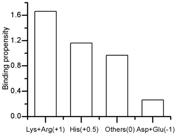
Plot of binding propensity vs. amino acids with different charges (shown in the parentheses).

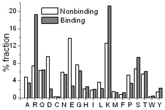
Composition of the neighbors

We found a higher composition of Arg and Lys (positively charged) around binding residues than around non-binding ones (Figure 2). Similarly, non-binding residues had a much higher fraction of negatively charged Asp and Glu in their vicinity than binding residues. These observations legitimize the fact that the neighboring residues also play a crucial role for a residue to bind to the DNA.

Figure 2.

Composition of the neighboring residue around binding and non-binding residues.

Occurrence in a cationic patch

The overlap of the binding and non-binding residues with large positive potential patches on the protein surface was determined. We found that around 45% of the binding residues are included in at least one of the four largest patches (Figure 3). On the other hand, 80% of the non-binding residues are not present in any of the four patches. This shows that the location of a positive potential patch can be a good first pass for identification of binding interface on the molecular surface.

Figure 3.

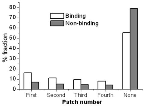
Fractions of binding and non-binding residues overlapping with large positive

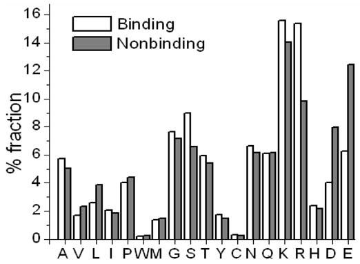
Identity Vector

Noticeable differences were found in the composition of the binding and non-binding residues with respect to some residues (Figure 4). For example, more than 40% of the binding residues were either Arg or Lys and about one-quarter of the non-binding residues were either Asp or Glu. This indicates the importance of the identity of the residue.

Figure 4.

Composition of the binding and non-binding residues.

Other features

We found that binding and non-binding residues do not show contrasting behavior in terms of their solvent accessible surface area (Figure 5A). This is not surprising, as our dataset is composed of only surface residues (those that have more than 40% area exposed). Some noticeable differences were observed in case of average residue potential (Figure 5B). There was no significant contrast between binding and non-binding residues with regards to secondary structural state (Figure 6). These observations show that accessible surface area, average residue potential and secondary structure carry only marginal, if any, information about a residue binding to the DNA.

Figure 5.

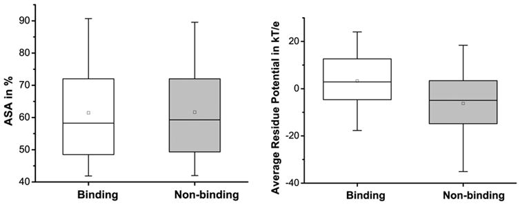
Box-and-whisker plots of the Accessible Surface Area (ASA) in % and average residue potential for binding and non-binding residues.

Figure 6.

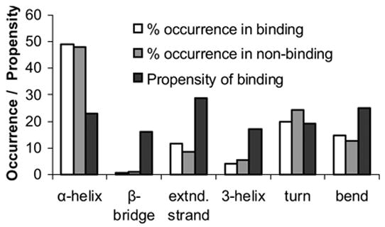
Plot of % occurrence of binding and non-binding residues in different secondary structures (white and gray bars) and propensity of binding for a residue present in that secondary structure (black bars). Propensity was obtained by dividing the number of binding residues present in a secondary structure by the total number of residues present in that secondary structure.

Combined performance of the features

We combined all the above mentioned features and built an SVM-based prediction model. The standard accuracy is defined as the ratio of number of correct predictions to the total number of predictions made. As mentioned earlier, there is an imbalance in the data in terms of number of positive and negative cases. Due to this imbalance, sensitivity (% of correct positive predictions) is outweighed by specificity (% of correct negative predictions). To even it out, we attached a weight of 2 to the data points belonging to the positive class. Net prediction, which is the arithmetic mean of sensitivity and specificity and attaches equal weights to both the datasets, was also reported. We tested Set I consisting of residues from 50 proteins with 5-fold CV while using Gaussian kernel. We achieved a balanced performance with an accuracy of 65.7% and a net prediction of 64.2% for cross-validation training. Corresponding sensitivity and specificity were 59.6% and 68.9%, respectively.

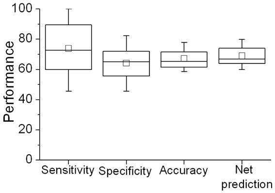
To evaluate the true performance of our prediction model, we used the SVM model built above to predict the class of every residue in Set II comprising of the remaining 37 proteins, which were not used during cross-validation with Set I. This resulted in a set of 37 metrics, one for every protein. Average accuracy value for this set was 66.47% (Figure 7), a value even a little higher than that of Set I. Similarly, average net prediction was also higher than that in Set I (66.48%). Mean sensitivity and specificity values were more balanced at 67.79% and 65.16%, respectively. The overall performance for this set was similar to that for the first set suggesting that the classification model trained on the first set holds well for the holdout set. We also plot the initial performance on the ROC curve (Figure 13, the filled square).

Figure 7.

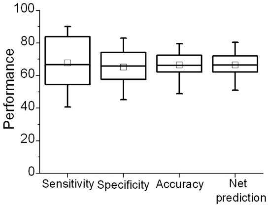
Box-plot of the performance for holdout evaluation performed over the set of 37 proteins.

Figure 13.

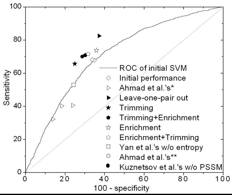
ROC curve showing the initial performance curve and the performance points after the refinement steps. The gray diagonal line corresponds to a completely random predictor. Other cited studies are by Kuznetsov et al. [14] and Yan et al. [15]. * Ahmad et al. [12]. ** Ahamd et al. [13].

To directly compare our results with similar results previously published [12] where leave-one-residue-out validation was used, we performed a similar test on our protocol. We randomly selected a pair of residues (one negative and one positive) and trained on the remaining set to form a model that was tested on the left-out pair. This was repeated 500 times with a random pair each time and an average performance was reported. We report a much higher and a more balanced performance with sensitivity and specificity at 62.8% and 82.6%. The improvement is also conspicuous from the ROC curve (empty and filled triangles, Figure 13).

II. Post-classification refinement

We have, so far, used the individual properties of the residues to classify them as binding or non-binding. We have not taken into account inter-residue location on the protein surface. Figure 8 shows a typical example of a protein with true positives, false negatives and false positives predicted by applying the above protocol. We inspected the location of predicted residues on the proteins and observed that some of the FNs are located in close vicinity of the TPs. Similarly, many of FPs (yellow balls) lie far apart from other positive predictions. So, we reasoned that distance-dependent refinement of the classification may boost the prediction performance.

Figure 8.

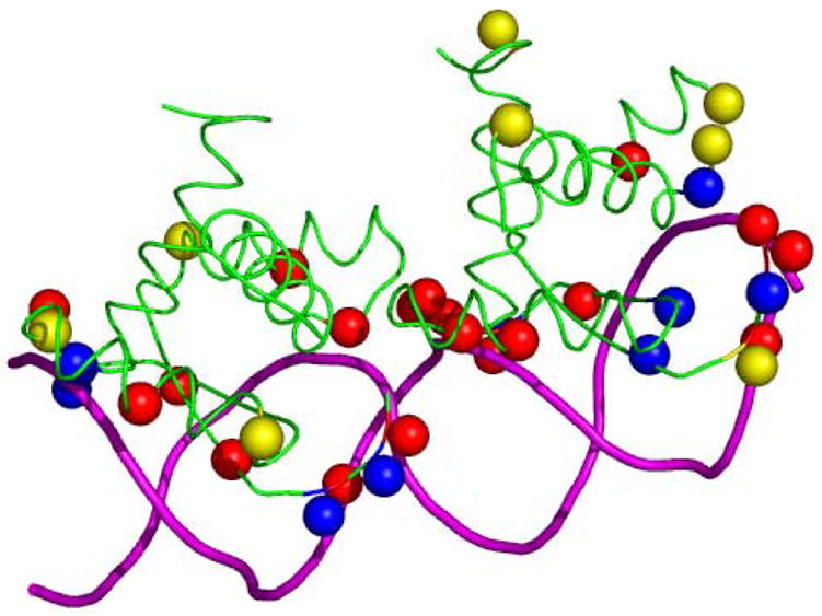
Prediction of DNA binding residues on the protein-DNA complex of arc repressor operator (PDB code 1par). DNA and protein are represented in tube representation in magenta and green, respectively. True positives, false negatives and false positives are represented by ball representation (Cα atoms) in blue, red and yellow, respectively.

Enrichment

We first added more residues to the list of positively predicted residues (TP+FP) using a neighbor criterion. We calculated the number of neighbors around FN, FP and TP. The underpinning idea was to label residues as positive that were previously classified as negative, if they have more than a certain number of positively classified residues within a cutoff, which was empirically chosen to be 9Å.

Figure 9 plots the fraction of TP, TN and FN with different number of neighbors within 9Å for the testing set. The cutoff for the number of neighbors is set at 3 where the fraction of TN becomes smaller than both TP and FN. All residues predicted to be negative that had 3 or more positively predicted residues within 9Å were classified as binding residues. With this first step of refinement, sensitivity increased by 6% to 73.8% (Figure 10). Net prediction also rose to 69% and accuracy to 67.36%. Specificity decreased by only 1% to 64.15%, which is not surprising, given that labeling more residues as positives is expected to include some false positives, hence decreasing specificity. The increment in the prediction performance is indicated on the ROC curve by an upward movement of the performance point (Figure 13, filled square to empty star). This movement is mainly due to an increase in sensitivity.

Figure 9.

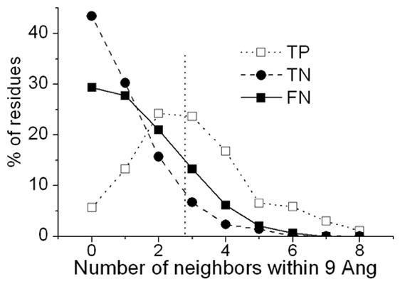
Number of positively predicted neighbors within 9Å against the fraction of different kinds of residues: true positives (TP), true negatives (TN) and false negatives (FN).

Figure 10.

Performance after enrichment. Negatively predicted residues having more than 3 positively predicted residues within 9 Å around them were labeled positive, hence increasing sensitivity.

Trimming

In another step of refinement, we removed the residues that were far away from any positively predicted residue. We calculated the distance of every positively-predicted residue from every other such residue. If the minimum of this set of distances was greater than 10Å, this residue was labeled as negative. This step discards the false positives that lie isolated from any positively predicted residue. With this step, mean specificity increased by 10% to 75.1%, whereas mean sensitivity decreased only by 2% resulting in a rise of 7% accuracy to 73.72% (Figure 11). Net prediction also increased by 4% to 70.41% as compared to the performance prior to any refinement. The improvement in the performance is also indicated on the ROC curve by a movement towards the left due to an increase in specificity (Figure 13, filled square to filled star).

Figure 11.

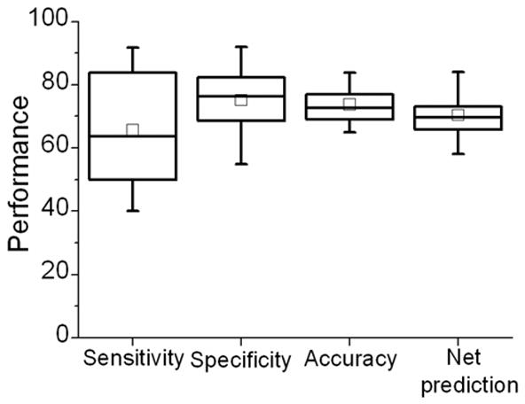
Performance after trimming by removing residues if the minimum distance from any positively predicted residue was greater than 10Å.

Trimming and enrichment in succession

We then applied the two steps of refinement in succession: trimming followed by enrichment (T+E) and enrichment followed by trimming (E+T). With these two steps trying to increase their respective performance criterion (specificity for trimming and sensitivity for enrichment), a higher and more balanced performance is expected. Indeed, a more balanced performance between sensitivity and specificity was registered (Figure 12 and Table 1).

Figure 12.

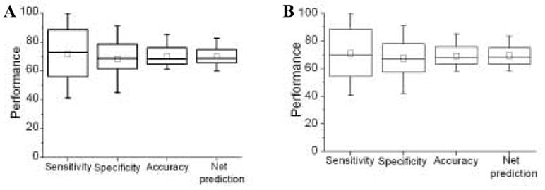
Performance after enrichment followed by trimming (A) and trimming followed by enrichment (B).

Table 1.

Performance for different datasets and after refinement

	Sensitivity	Specificity	Accuracy	Net Prediction
Initial performance (set I)	59.6%	68.9%	65.7%	64.2%
Initial performance (set II)	67.79%	65.16%	66.47%	66.48%
Enrichment (set II)	73.8%	64.15%	67.36%	69.00%
Trimming (set II)	65.73%	75.1%	73.72%	70.41%
Enrichment + Trimming (set II)	71.65%	68.38%	70.10%	70.02%
Trimming + Enrichment (set II)	70.9%	69.8%	70.8%	70.35%

In E+T, an accuracy of 70.10% was achieved with sensitivity and specificity at 71.65% and 68.38%. Similarly for T+E, sensitivity and specificity registered were 70.9% and 69.8%, accuracy being 70.8%. In both the cases, the second step reduces the imbalance in performance introduced due to the first step. The overall improvement of these steps combined is reflected by an upper-left movement of the performance point on the ROC curve (Figure 13, empty diamond to empty/filled pentagons). From the curve it is clear that application of both refinement steps in succession results in both high and more balanced performance. It can also be seen from the graph that there is not much difference between the final performances regardless of the order of these steps. Initially the two points move in their respective directions (enrichment towards the left and trimming towards the top), but after the second step they both converge very close to each other. The final performance after these post-processing steps is very similar to that reported in a previous study [14] where ~71% accuracy was achieved with similar sensitivity and specificity (Figure 13). It should be noted that for a fair comparison, the performance in presented here without using any evolutionary information is used is compared to the performance in that study before adding conservation profile as input. Similarly, our performance before post-classification refinement is almost identical as that reported in Yan et al. [15] without using any entropy as is shown by the point corresponding to their performance lying on our initial ROC curve. Although they had used a slightly different definition of specificity we calculated their specificity according to our definition using the values of their accuracy, specificity, sensitivity and the number of total residues. We report a higher performance than the previous two studies by Ahmad et al.[12,13].

III. Identification of binding residues on novel structural classes/folds

We wanted to see how our prediction protocol performed on predicting residues on some new structural folds. We used the classification proposed by Thornton lab [1] where a set of 240 protein-DNA complexes was divided into eight major groups on the basis of their functions, structures and binding interactions. Most of the proteins in this study were present in this set. The proteins in our set that were not in the list of 240 complexes were examined manually and assigned a class using the same classification rules. Our training set did not have any proteins from one class, the β-sheet, whereas the testing set had four proteins from this class with a total of 498 residues from these four proteins. The above protocol gave an admirable performance on these four proteins after post-processing; average sensitivity and specificity was 67.4% and 69.6%, respectively. Accuracy was 69.3% and net prediction of 68.5% was reported. This shows that our protocol can also identify residues embedded in novel structural motifs that it has not seen during training so far.

IV. Prediction of DNA-binding proteins

Another useful application of DNA-binding residues prediction would be the identification of proteins that bind to DNA. We tried to examine if predictions about a protein’s DNA-binding function can be made based on the number of DNA-binding sites predicted. Positive dataset for this evaluation consists of the 37 DNA-binding proteins from set II used above. For negative dataset, a list of 205 non-binding proteins was obtained from a previous related study [22]. The same features were generated for all the surface residues on the non-binding proteins. The classification model built above was used to classify these residues as binding or non-binding and the total number of residues predicted to be binding was determined for each protein.

We plotted the fraction of proteins against the number of positively-predicted residues on their surface as a bin distribution (with a bin-width of 5 residues) (Figure 14A). Based on the plot, a tentative cutoff was chosen at 35 residues, meaning that all proteins with 35 or more residues predicted to be binding are classified as DNA-binding. With this cutoff, sensitivity and specificity for protein-level prediction were 63.1% and 71.6%, respectively. Accuracy was around 69.7% and net prediction was 67.3%. These values are a little higher than accuracy and net prediction reported in Ahmad et al. [12] where DNA-binding residues were used to predict DNA-binding proteins with 64.5% accuracy 66.1% net prediction using 3-fold cross-validation. We also carried out post-classification refinement for non-binding proteins in a fashion similar to binding proteins. After post-processing, accuracy increased to 78.2% and net prediction increased to 74.4% (Figure 14B). These values suggest that number of binding residues predicted on a protein surface can be a good first pass to predict its DNA-binding function. Furthermore the distance-based post-prediction refinement can augment the DNA-binding protein prediction performance.

Figure 14.

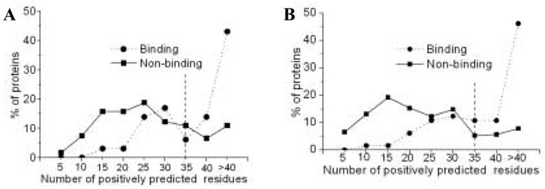
Distinction between DNA-binding and DNA-non-binding proteins on the basis of residues predicted to be binding before (A) and after (B) post-processing. Y-axis plots the fraction of proteins falling in each bin.

4. Discussion

Over the last three decades since the discovery that lac operon was regulated by a protein, human knowledge about protein-DNA interactions has soared [2–4,35]. Examination of solved protein-DNA complexes has shown a stereochemical complementarity between various factors involved in the formation of the complex. However, the mechanisitics and energetics of protein-DNA interactions are sparsely understood because protein-DNA interactions are both flexible and redundant. Recognition of probable binding sites both on the protein and the DNA will go a long way in diagnosing the basis of these interactions. Their discovery can help lead subsequent works such as site-directed mutagenesis and constrained macromolecular docking. Prediction of functional sites to act as filters in a predictive scheme for docking can be as effective as manually introducing biological constraints.

In the present work we have built up a framework for automated recognition of DNA-binding sites on protein surface. The method is based on training kernel-based SVM to identify binding sites on the basis of a number of their features. We have also implemented a distance-based refinement of the classification given by the SVM. With these two methods in alliance, we could achieve a more balanced success with mean sensitivity and specificity values at 71.3% and 69.3%, respectively. Net prediction and accuracy obtained are around 70.5%. The improvement in performance after post-processing is also apparent from the ROC curve that shows a north-west movement from the initial performance curve (Figure 13).

In a related study, Jones et al. [25] analyzed surface patches for electrostatic potential, accessibility and other properties and ranked these patches on the basis of the scores. They used a fixed patch size of 10 residues and any protein having 7 or more residues overlapping with the actual binding interface was deemed to be correctly classified. This way they could correctly predict sites for 68% of the proteins. Since their accuracy is at the protein-level, there is no direct comparison between their values and values reported in this paper, which are at the residue level.

We have also shown that identification of DNA-binding sites can also assist in prediction of DNA-binding behavior of a protein. This is similar in spirit to other studies that assign functions to a protein on the basis of functional sites discovered on its surface, such as protein-protein and protein-DNA interaction sites [11]. Relevant preliminary results presented above shows that the number of predicted DNA-binding residues promises to be a good descriptor for identification of DNA-binding proteins. It is also reasonable to believe that in combination with other applicable descriptors, prediction performance can be pushed further.

As accentuated in this and other previous studies [1,12–15], one of the main predicaments in automated identification of DNA-binding residues, is a proportionately low value of sensitivity. This probably emanates from a low fraction of binding residues in comparison to non-binding ones on the molecular surface. This discrepancy tends to attach a higher moment to negative cases and, in the process, introduce a number of false negatives. Apart from adopting a way of removing this inequality by pre-filtering some of the residues, a possible channel of improving the prediction power would be addition of more features of the residues that can distinguish the binding residues from the non-binding ones. Another impediment in the prediction of DNA-binding residues stems from the fact that proteins do not bind to the DNA in isolation. Rather, there is a whole set of multiple regulatory factors, often interacting cooperatively and sometimes even competitively. Therefore, a protein binds to the DNA in a fashion that is commodious to all the other agents, which might not be the same as in isolation. Moreover, the nature of protein-DNA binding is very intricate and involves many types of interactions: hydrogen bonds, electrostatic and hydrophobic interactions, effects of water-extrusion-related ‘indirect readout’, and DNA bending and twisting [36]. Combination of these interactions makes the task of predicting binding sites on the basis of some apparent descriptors challenging. An ideal tool for identification of DNA-binding sites will perhaps need to take into account the synergetic effects of all these interactions and numerous other factors that mediate interactions both between the protein and the DNA, and among DNA-binding proteins themselves. Nevertheless, an important first step in this direction is to examine the potential features for their ability to reveal the binding sites. Various features studied in this work show differing prediction power. We believe that the process of adding more features to this end will be a continuous process for sometime in the future as and when human knowledge about the determinants behind selection of binding sites advances.

References

- 1.Luscombe NM, Austin SE, Berman HM, Thornton JM. An overview of the structures of protein-DNA complexes. Genome Biol. 2000;1:1–37. doi: 10.1186/gb-2000-1-1-reviews001. [DOI] [PMC free article] [PubMed] [Google Scholar]
- 2.Jones S, Heyningen Pv, Berman HM, Thornton JM. Protein-DNA interactions: A Structural Analysis. J Mol Biol. 1999;287:877–896. doi: 10.1006/jmbi.1999.2659. [DOI] [PubMed] [Google Scholar]
- 3.Ren B, et al. Genome-wide location and function of DNA binding proteins. Science. 2000;290:2306–9. doi: 10.1126/science.290.5500.2306. [DOI] [PubMed] [Google Scholar]
- 4.Stormo GD. DNA binding sites: representation and discovery. Bioinformatics. 2000;16:16–23. doi: 10.1093/bioinformatics/16.1.16. [DOI] [PubMed] [Google Scholar]
- 5.Stormo G. DNA binding sites: representation and discovery. Bioinformatics. 2000;16:16–23. doi: 10.1093/bioinformatics/16.1.16. [DOI] [PubMed] [Google Scholar]
- 6.Day WH, McMorris FR. Critical comparison of consensus methods for molecular sequences. Nucleic Acids Research. 1992;20:1093–9. doi: 10.1093/nar/20.5.1093. [DOI] [PMC free article] [PubMed] [Google Scholar]
- 7.Stormo GD, Schneider TD, Gold L, Ehrenfeucht A. Use of the 'Perceptron' algorithm to distinguish translational initiation sites in E. coli. Nucleic Acids Res. 1982;10:2997–3011. doi: 10.1093/nar/10.9.2997. [DOI] [PMC free article] [PubMed] [Google Scholar]
- 8.Schneider TD, Stormo GD, Gold L, Ehrenfeucht A. Information content of binding sites on nucleotide sequences. J Mol Biol. 1986;188:415–31. doi: 10.1016/0022-2836(86)90165-8. [DOI] [PubMed] [Google Scholar]
- 9.Sarai A, Kono H. Protein-DNA recognition patterns and predictions. Annu Rev Biophys Biomol Struct. 2005;34:379–98. doi: 10.1146/annurev.biophys.34.040204.144537. [DOI] [PubMed] [Google Scholar]
- 10.Ruvkun GB, Ausubel FM. A general method for site-directed mutagenesis in prokaryotes. Nature. 1981;289:85–8. doi: 10.1038/289085a0. [DOI] [PubMed] [Google Scholar]
- 11.Aloy P, Querol E, Aviles FX, Sternberg MJE. Automated Structure-based Prediction of Functional Sites in Proteins: Applications to Assessing the Validity of Inheriting Protein Function from Homology in Genome Annotation and to Protein Docking. J Mol Biol. 2001;311:395–408. doi: 10.1006/jmbi.2001.4870. [DOI] [PubMed] [Google Scholar]
- 12.Ahmad S, Gromiha MM, Sarai A. Analysis of DNA-binding proteins and their binding residues based on composition, sequence and structural information. Bioinformatics. 2004;20:477–486. doi: 10.1093/bioinformatics/btg432. [DOI] [PubMed] [Google Scholar]
- 13.Ahmad S, Sarai A. PSSM-based prediction of DNA binding sites in proteins. BMC Bioinformatics. 2005;6:33. doi: 10.1186/1471-2105-6-33. [DOI] [PMC free article] [PubMed] [Google Scholar]
- 14.Kuznetsov IB, Gou Z, Li R, Hwang S. Using evolutionary and structural information to predict DNA-binding sites on DNA-binding proteins. Proteins. 2006;64:19–27. doi: 10.1002/prot.20977. [DOI] [PubMed] [Google Scholar]
- 15.Yan C, Terribilini M, Wu F, Jernigan RL, Dobbs D, Honavar V. Predicting DNA-binding sites of proteins from amino acid sequence. BMC Bioinformatics. 2006;7:262. doi: 10.1186/1471-2105-7-262. [DOI] [PMC free article] [PubMed] [Google Scholar]
- 16.Vapnik V, Cortes C. Support vector networks. Machine Learning. 1995;20:273–293. [Google Scholar]
- 17.Ding CH, Dubchak I. Multi-class protein fold recognition using support vector machines and neural networks. Bioinformatics. 2001;17:349–58. doi: 10.1093/bioinformatics/17.4.349. [DOI] [PubMed] [Google Scholar]
- 18.Dubchak I, Muchnik I, Mayor C, Dralyuk I, Kim SH. Recognition of a protein fold in the context of the Structural Classification of Proteins (SCOP) classification. Proteins. 1999;35:401–7. [PubMed] [Google Scholar]
- 19.Langlois RE, Diec A, Perisic O, Dai Y, Lu H. Improved protein fold assignment using support vector machines. International Journal of Bioinformatics Research and Applications. 2006;1:319. doi: 10.1504/IJBRA.2005.007909. [DOI] [PubMed] [Google Scholar]
- 20.Brown MP, Grundy WN, Lin D, Cristianini N, Sugnet CW, Furey TS, Ares M, Jr, Haussler D. Knowledge-based analysis of microarray gene expression data by using support vector machines. Proc Natl Acad Sci U S A. 2000;97:262–7. doi: 10.1073/pnas.97.1.262. [DOI] [PMC free article] [PubMed] [Google Scholar]
- 21.Jaakkola T, Diekhans M, Haussler D. Using the Fisher kernel method to detect remote protein homologies. Proc Int Conf Intell Syst Mol Biol. 1999:149–58. [PubMed] [Google Scholar]
- 22.Bhardwaj N, Langlois RE, Zhao G, Lu H. Kernel-based machine learning protocol for recognizing DNA-binding proteins. Nucleic Acid Research. 2005;33:6486–6493. doi: 10.1093/nar/gki949. [DOI] [PMC free article] [PubMed] [Google Scholar]
- 23.Bhardwaj N, Stahelin RV, Langlois RE, Cho W, Lu H. Structural bioinformatics prediction of membrane-binding proteins. J Mol Biol. 2006;359:486–95. doi: 10.1016/j.jmb.2006.03.039. [DOI] [PMC free article] [PubMed] [Google Scholar]
- 24.Stawiski EW, Gregoret LM, Mandel-Gutfreund Y. Annotating Nucleic Acid-Binding Function Based on Protein Structure. J Mol Biol. 2003;326:1065–1079. doi: 10.1016/s0022-2836(03)00031-7. [DOI] [PubMed] [Google Scholar]
- 25.Jones S, Shanahan HP, Berman HM, Thornton JM. Using electrostatic potentials to predict DNA-binding sites on DNA-binding proteins. Nucleic Acids Res. 2003;31:7189–7198. doi: 10.1093/nar/gkg922. [DOI] [PMC free article] [PubMed] [Google Scholar]
- 26.Tsuchiya Y, Kinoshita K, Nakamura H. Structure-based prediction of DNA-binding sites on proteins using the empirical preference of electrostatic potential and the shape of molecular surfaces. Proteins. 2004;55:885–94. doi: 10.1002/prot.20111. [DOI] [PubMed] [Google Scholar]
- 27.Word JM, Lovell SC, Richardson JS, Richardson DC. Asparagine and glutamine: using hydrogen atom contacts in the choice of side-chain amide orientation. J Mol Biol. 1999;285:1735–47. doi: 10.1006/jmbi.1998.2401. [DOI] [PubMed] [Google Scholar]
- 28.Kabsch W, Sander C. Dictionary of protein secondary structure: pattern recognition of hydrogen-bonded and geometrical features. Biopolymers. 1983;22:2577–637. doi: 10.1002/bip.360221211. [DOI] [PubMed] [Google Scholar]
- 29.Honig B, Sharp K, Gilson M. Electrostatic interactions in proteins. Prog Clin Biol Res. 1989;289:65–74. [PubMed] [Google Scholar]
- 30.Sharp KA, Honig B. Electrostatic interactions in macromolecules: theory and applications. Annu Rev Biophys Biophys Chem. 1990;19:301–32. doi: 10.1146/annurev.bb.19.060190.001505. [DOI] [PubMed] [Google Scholar]
- 31.Jayaram B, Sharp KA, Honig B. The electrostatic potential of B-DNA. Biopolymers. 1989;28:975–93. doi: 10.1002/bip.360280506. [DOI] [PubMed] [Google Scholar]
- 32.Brooks B, Bruccoleri RE, Olafson B, States D, Swaminathan S, Karplus M. CHARMM: a program for macromolecular energy, minimization, and dynamics calculations. J Comput Chem. 1983;4:187–217. [Google Scholar]
- 33.Henikoff S, Henikoff JG. Amino acid substitution matrices from protein blocks. Proc Natl Acad Sci U S A. 1992;89:10915–9. doi: 10.1073/pnas.89.22.10915. [DOI] [PMC free article] [PubMed] [Google Scholar]
- 34.Chang C-C, Lin C-J. LIBSVM: A library for support vector machines. 2001 Software available at http://www.csie.ntu.edu.tw/~cjlin/libsvm.
- 35.Gilbert W, Maxam A. The nucleotide sequence of the lac operator. Proc Natl Acad Sci U S A. 1973;70:3581–4. doi: 10.1073/pnas.70.12.3581. [DOI] [PMC free article] [PubMed] [Google Scholar]
- 36.Mirny LA, Gelfand MS. Structural analysis of conserved base pairs in protein-DNA complexes. Nucleic Acids Res. 2002;30:1704–11. doi: 10.1093/nar/30.7.1704. [DOI] [PMC free article] [PubMed] [Google Scholar]