Biological Parametric Mapping: A Statistical Toolbox for Multi-Modality Brain Image Analysis

Abstract

In recent years multiple brain MR imaging modalities have emerged; however, analysis methodologies have mainly remained modality specific. In addition, when comparing across imaging modalities, most researchers have been forced to rely on simple region-of-interest type analyses, which do not allow the voxel-by-voxel comparisons necessary to answer more sophisticated neuroscience questions. To overcome these limitations, we developed a toolbox for multimodal image analysis called biological parametric mapping (BPM), based on a voxel-wise use of the general linear model. The BPM toolbox incorporates information obtained from other modalities as regressors in a voxel-wise analysis, thereby permitting investigation of more sophisticated hypotheses. The BPM toolbox has been developed in MATLAB with a user friendly interface for performing analyses, including voxel-wise multimodal correlation, ANCOVA, and multiple regression. It has a high degree of integration with the SPM (statistical parametric mapping) software relying on it for visualization and statistical inference. Furthermore, statistical inference for a correlation field, rather than a widely-used T-field, has been implemented in the correlation analysis for more accurate results. An example with in-vivo data is presented demonstrating the potential of the BPM methodology as a tool for multimodal image analysis.

Introduction

Functional MR imaging (fMRI) has revolutionized the field of neuroscience and has emerged as a widely used research tool for the probing of neural processes. It has evolved predominantly using BOLD (Blood Oxygen level Dependent) fMRI techniques (Ogawa, et al. 1990). Over the last several years, additional imaging modalities have emerged, including diffusion tensor imaging (DTI), perfusion imaging, T2 mapping, 3D spectroscopic imaging, and a variety of anatomic-based methods such as voxel-based morphometry (VBM). There is, however, a relative lack of available multimodal image analysis methodologies. That is, analysis for each form of functional imaging data has mainly proceeded to develop specific to that imaging modality. Despite this, there has been some work in multi-modality massively univariate analyses. For example, Richardson et al. (1997) proposed a univariate technique, a voxel-wise group-by-modality interaction analysis based on SPM (Statistical Parametric Mapping), and applied to the analysis of PET and MRI data recorded from normal and epileptic subjects. In another univariate approach (Pell, et al. 2004), a conjunction analysis (Friston, et al. 1999) was applied to voxel-based morphometry (VBM) and T2-relaxometry data to assess the degree of concurrent changes in both data sets. A non-parametric method has recently been proposed based on the use of combining functions and permutation testing that is able to detect not only areas of concurrent changes but also disassociated changes across modalities (Hayasaka, et al. 2006). None of these massively univariate approaches, however, can explicitly model changes in one imaging modality as a function of another modality. Only recently a data-driven method has been proposed as an exploratory tool for multiple modality imaging based on independent component analysis (ICA) (Calhoun, et al. 2006) .

In this technical note we describe an approach to multimodal integrative image analysis using the biological parametric mapping (BPM) software package. The BPM software allows probing of neuroimaging data using information from other functional or structural imaging modalities. The major conceptual difference between a BPM analysis and a conventional SPM (statistical parametric mapping)-style analysis is in the use of biological information, such as choline concentration or tissue anisotropy, obtained from one or more imaging modalities, as regressors in an analysis of another imaging modality in a massively-univariate fashion. For example, a BPM analysis can determine if changes in metabolite levels (from 3D spectroscopy) or fractional anisotropy (in diffusion tensor data) correlate with activations in an fMRI experiment and vice-versa. The statistical concepts embodied in a BPM-style analysis are not novel, and can be found in any general textbook of statistics. However, the application of these methods to neuroimaging research provides a powerful tool for hypothesis testing and discovery that otherwise is not available.

We describe the BPM toolbox that incorporates correlation, ANCOVA and multiple regression analyses of multimodal imaging data sets. Here, we utilize the toolbox to analyze invivo data. The BPM toolbox uses the theoretical framework behind the widely used SPM methodology: the general linear model (GLM) (Friston, et al. 1995) for statistical estimation, and random field theory (RFT) (Worsley, et al. 1996) or false discovery rate (FDR) (Benjamini and Hochberg 1995; Genovese, et al. 2002) for statistical inference. In addition to the RFT-based inference on T- and F-images, we have implemented RFT-based inference for correlation images (Cao and Worsley 1999) in our correlation analysis, which is more appropriate in this context.

Materials and Methods

BPM allows solving a GLM with a different design matrix in each voxel (Figure 1). The difference in design matrices is due to allowing image data covariates. Supported analyses include ANCOVA, correlation, and multiple regression. The BPM toolbox was developed entirely in MATLAB (MathWorks; Natick, MA, USA) as an open source package. It was designed to only use routines available in a standard Matlab distribution and does not require any additional Matlab toolboxes. The BPM toolbox has a high degree of integration with SPM package (Wellcome Department of Imaging Neuroscience, London, UK) and employs basic SPM I/O (input/output) functions for reading and writing image data in Analyze (Mayo Foundation, Rochester, MN) and NIfTI (Neuroimaging Informatics Technology Initiative, www.nifti.nimh.nih.gov) formats. It is compatible with both SPM2 and SPM5.

Figure 1.

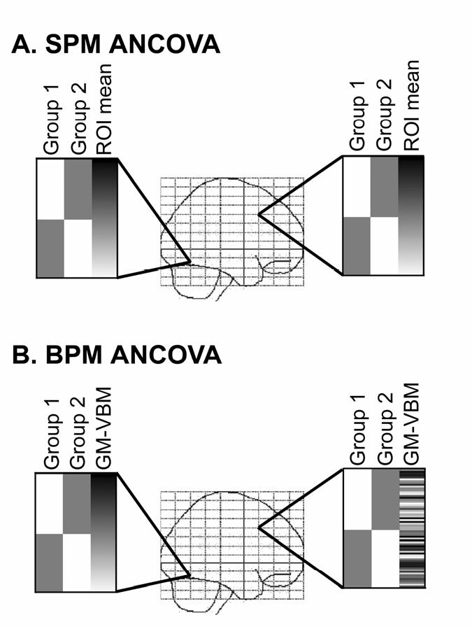
BPM Design Matrix. In the hypothetical ANCOVA models demonstrated here the first 2 columns represent 2 hypothetical study populations and column 3 represents a nuisance regressor. This third column demonstrates the difference between a traditional SPM analysis and the BPM approach. A). In a standard SPM-style analysis all voxels have the same design matrix, where the nuisance regressor represents some scalar value (e.g. mean gray matter volume within an ROI). Note that the model is exactly the same in the different brain regions. B). In a BPM analysis, each voxel has a unique design matrix. In the example shown here, the values in column 3 represent the corresponding gray matter volume voxel-values. Since the gray matter volume values are different in various brain regions, the design matrix is unique at each voxel.

The main program is called from the Matlab command line by entering wfu_bpm. This invokes a user-friendly GUI (graphic user interface) with three main options (BPM Analysis, Contrast Manager, and SPM Insertion Tool). Each of these is described in detail below (Figure 2). Alternatively, non-interactive operation of the toolbox is possible by supplying command-line parameters.

Figure 2.

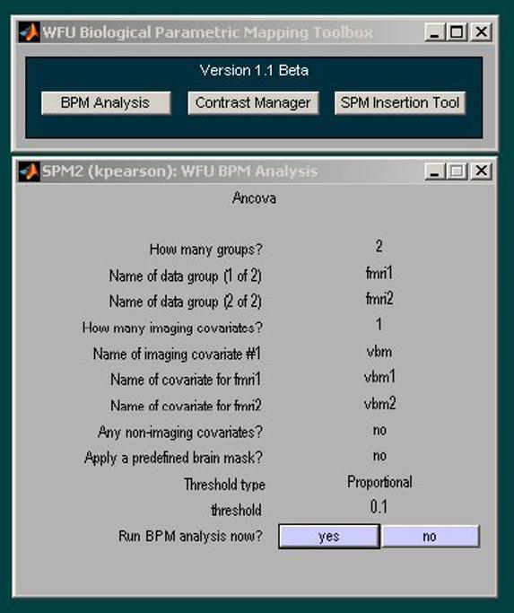
BPM GUI. The 3 main BPM GUI options are shown at the top. In this example, a BPM ANCOVA analysis was performed for 2 groups with a primary modality of fMRI and a single imaging covariate of VBM.

BPM Analysis

The BPM analysis option initiates the main GLM statistical estimation module. It permits the user to enter the information needed to carry out the specific statistical procedure that includes: type of analysis (correlation, ANOVA, ANCOVA, and multiple regression), number of imaging modalities (e.g., fMRI and VBM), and number of non-imaging regressors (see figure 2). Logic is built into the GUI to limit responses based on previous selections (e.g., only 2 modalities are allowed if correlation is chosen). The user then selects the images for each portion of the analysis. For simplicity, these can be provided as text files containing a list of the respective image filenames. The program then constructs the design matrix and performs the computations on a voxel-wise basis, producing parameter estimates that are used later in the contrast manager to generate T-maps, correlation maps, or F-maps.

The user is also prompted to enter a mask of the brain region in order to restrict the statistical analysis. If the user is unable to provide a mask, the BPM software will generate a default mask using the main imaging modality (the first imaging modality provided). It is computed as the intersection of the individual masks generated for each subject image in the first level analysis. It can optionally be computed using a proportional threshold in relation to the mean value of the voxel intensities or by using a user-supplied threshold.

A BPM structure is created containing analysis specific information (i.e., file names, working directory and computational parameters). This structure is saved in a BPM.mat file that will later be used as the primary input for the contrast manager and the SPM insertion tool.

Contrast Manager

A BPM contrast manager (Figure 3) allows the user to specify contrasts and generate statistic images. The contrast manager prompts for the BPM.mat file and loads information about the fitted GLM saved during the analysis phase. The user can then enter the contrast to be tested. In the case of an ANOVA or an ANCOVA, the contrast is a vector (T-contrast) and a T-map is generated. In the case of multiple regression, the contrast currently allowed is a matrix (F-contrast). In the correlation analysis, positive and negative correlation images are generated.

Figure 3.

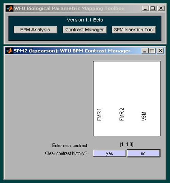
The BPM contrast widget provides a simple intuitive interface for entering user-defined contrasts. In this example, a contrast weight of (1 -1 0) is applied for FMRI group 1, FMRI group 2, and the VBM imaging covariate, respectively.

One issue to be considered in BPM analyses is the estimability of the contrast at each voxel. A contrast c^Tβ is estimable at a given voxel if c is a linear combination of the rows of X (Frackowiak, et al. 2003). In conventional SPM analyses this property needs to be evaluated only once for a user defined contrast. In a BPM analysis however, since the design matrix varies across voxels, there can potentially be problems with the estimability of a given contrast in some subsets of voxels. In the case of T-contrasts we have thus far been using contrast vectors with weights that sum to zero that are inherently estimable. For more general types of contrasts a voxel-wise check for estimability may need to be introduced. In the case of F-contrasts we currently only allow those contrast matrices that define a partition of the original design matrix into two subsets of regressors (X = [X₁ X ₂]). This tests whether a simpler model, composed of a subset of user specified regressors X₁ from the original design matrix, gives an acceptable fit to the data (H ₀: β₁ = 0, whereβ₁ is a vector of parameters associated to a GLM defined by X₁) (Frackowiak, et al. 2003).

SPM Insertion Tool

The BPM toolbox relies on the SPM software for statistical inference and visualization. An SPM insertion tool was developed for exporting the statistical maps created by BPM to the SPM environment. This program takes any T-map or F-map and creates appropriate files to allow the map to be viewed and thresholded using SPM. Parameters required by the RFT such as degrees of freedom and smoothness of the maps are automatically computed and stored in the BPM.mat file as part of the BPM analysis. Figure 4 demonstrates an example of a BPM T-map displayed within the SPM environment.

Figure 4.

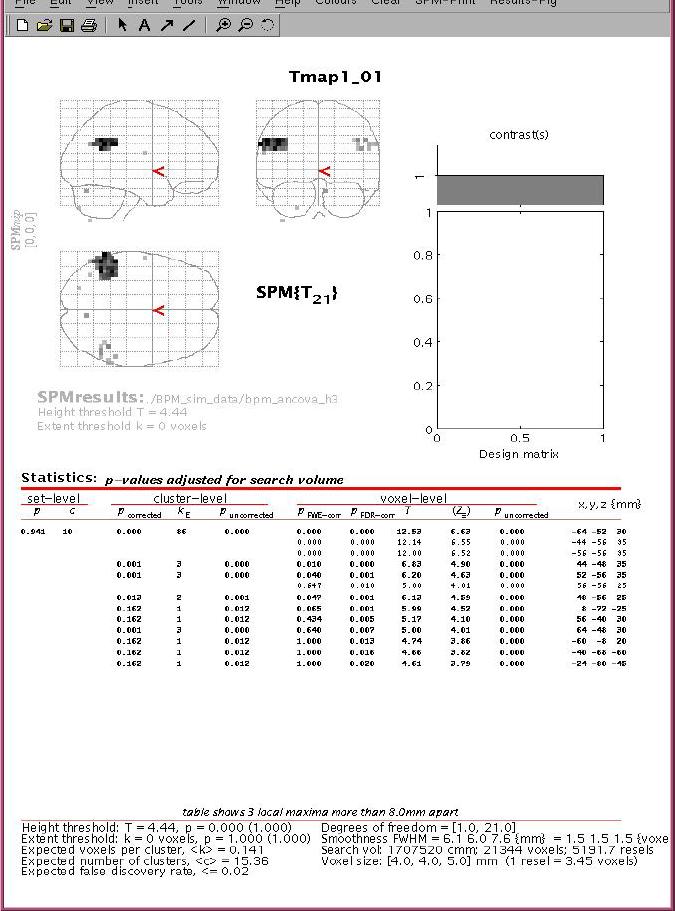
BPM T-map displayed in the SPM environment with SPM visualization and inference tools.

For a statistical analysis of correlation images, the random field results for a homologous correlation field (Cao and Worsley 1999; Cao and Worsley 2001) have been implemented. This was done by modifying the RFT component of the SPM package. This modification enables a statistical inference directly based on a correlation image, rather than the t-transformation. Although such a transformation produces voxel values distributed as a t-distribution, the resulting image does not represent a t random field in a strict sense (Cao and Worsley 1999). Details on the p-value calculation for a correlation field are found in the Appendix.

In Vivo Example

Data from 13 adult normal readers and 13 adult dyslexic readers were acquired as part of a larger study that will be reported in full elsewhere. The fMRI paradigm was designed to identify brain regions responsible for visual-auditory sensory integration using a phonemegrapheme matching task.

Functional imaging was performed using multislice gradient-echo echo planar imaging (TR=2500, TE=40 msec) on a 1.5-T MR scanner with Twin-speed gradients and a birdcage head coil (GE Medical Systems, Milwaukee, WI). Acquisition parameters included a field of view of 24 cm (frequency) x15 cm (phase), and an acquisition matrix of 64x40 (28 slices, 5 mm thickness, no gap). High-resolution T1 anatomic images were also obtained in the axial plane using a 3D spoiled gradient echo (3D-SPGR) sequence with the following parameters: matrix, 256 x 256; field of view, 24 cm; section thickness, 3 mm with no gap between sections; number of sections, 60; in-plane resolution, 0.9375 x 0.9375 mm.

The preprocessing steps for voxel based morphometry were performed within SPM using the structural high-resolution T1 images for each subject as previously described (Ashburner and Friston 2000). Briefly, the VBM preprocessing steps include stereotaxic normalization, segmentation into grey, white and CSF partitions, smoothing, and logit transformation. The T1 anatomical images were normalized to the MNI (Montreal Neurological Institute) template.

Functional image sets were pre-processed using the SPM package. The functional data sets were motion corrected (intra-run realignment) using the first image as the reference. The functional data sets were then normalized to MNI space and smoothed using a 10 mm FWHM (Full Width at Half Maximum) Gaussian smoothing kernel.

The in-vivo fMRI data was entered into an ANOVA analysis using the BPM software, testing for differences between the dyslexic and normal groups. An ANOVA was also performed on the in-vivo VBM data testing for differences in these 2 groups. Although these ANOVA analyses could have also been performed using existing software (e.g., SPM), the BPM software was used to demonstrate this functionality. An ANCOVA was then performed using the fMRI data as the primary modality and the corresponding VBM data as the imaging regressor. Furthermore, the correlation between the BOLD signal and gray matter volume (GMV) was calculated on a voxel-by-voxel basis with the BPM correlation model.

Results

Figure 5 shows the results of the in-vivo fMRI ANOVA, VBM ANOVA, and ANCOVA analyses comparing normal and dyslexic subjects (Dyslexic>Normal), as well as the correlation analysis results. The statistical maps were thresholded at p < 0.0025 and corrected for cluster extent at p<0.05. In the ANOVA performed between the two groups of subjects, a focus of activation is present (Figure 5 a) in the left temporo-occipital area (Brodmann area 37), representing increased activity in the dyslexic readers performing the visual-auditory matching task when compared with the normal readers. At the same axial slice level, the dyslexic readers show diminished GMV in an area that encompasses the region of fMRI activation differences (Figure 5 b).

Figure 5.

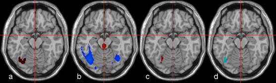
In-Vivo BPM results for a dyslexia study. Panel a represents ANOVA fMRI, panel b ANOVA VBM, panel c ANCOVA BPM, and panel d correlation analysis (all maps thresholded at p < 0.0025 uncorrected and displayed in neurologic convention). In panels a, b, and c, red and blue colors correspond to the contrasts (Dyslexic > Normal), (Normal>Dyslexic) respectively. In panel d, blue corresponds to negative association between fMRI and VBM. Left temporal activation (panel a) is regressed out after ANCOVA BPM (panel c). A negative association between the fMRI signal and local gray matter difference in the overlapping area is demonstrated in panel d (p<0.05 corrected for cluster-level using homologous correlation field).

For the ANCOVA, the VBM data was included as a regressor to evaluate the influence of the gray matter differences on the functional activity. The results demonstrate that the previously detected fMRI differences in the fMRI ANOVA are reduced to insignificance in all areas of overlap when the differences in gray matter volumes are taken into consideration (Figure 5 c). It should be noted that small regions of activation that do remain are not within the area representing anatomical group differences. In addition, the correlation analysis results (Figure 5 d) indicate a negative association between the fMRI signal and local gray matter difference in the overlapping area (p<0.05 corrected for cluster-level).

Discussion

In this paper we have described a method for performing SPM group analysis with image data as an independent variable using the BPM software package. It is a massively-univariate approach that utilizes the general linear model for statistical estimation and RFT or FDR for statistical inference. Although the BPM package is designed to take imaging data as covariates, it can also accept scalar dependent measures into the design matrix. The use of the SPM inference and visualization tools will make this tool immediately useful and familiar to a large portion of the neuroimaging community. At this time, the BPM package is not compatible with the SnPM package (SnPM Authors, the University of Michigan; Ann Arbor, MI, USA) for non-parametric analysis, although an extension to non-parametric methodologies is feasible. The computational demand for performing a BPM analysis is highly dependent on the size of the search region, the number of subjects, and the number of imaging covariates incorporated into the model. For the ANCOVA example provided here, using a single imaging covariate, computational demand is similar to a standard SPM analysis with a single column regressor. For larger analyses that incorporate multiple imaging regressors, performance increases can be achieved by implementing distributed grid computing with slice-wise or voxel-wise parcellation schemes.

Most fMRI analysis packages allow users to collapse an entire image data set or region of interest (ROI) into a single value (i.e. taking a mean value) and enter this value into a linear regression model. Although such analyses can be useful in controlling for image-based variables, results obtained from a BPM analysis and an ROI-based analysis are importantly distinct. The region-specific nature of the BPM analysis ensures that imaging metrics from one brain area (e.g. temporal lobe) are not meaninglessly regressed against data from another entirely disparate region of the brain (e.g. frontal lobe). BPM is also fundamentally different from a conjunction analysis (Friston, et al. 1999; Pell, et al. 2004). A conjunction analysis is used to determine common areas of activation in different data sets, but cannot be used to perform voxel-wise regression analysis between modalities.

The example provided here demonstrates some uses of this technique for the analysis of neuroimaging data. In the ANCOVA, group differences in functional activity were evaluated while controlling for gray matter volume. The analysis revealed that activity in the left temporooccipital area was explained by the differences in gray matter density in the same area. Moreover, the negative correlation between the fMRI signal and GM volume was demonstrated by the correlation analysis. Based on these findings, one can conclude that the reduced GM and increased BOLD activation are associated. Without a tool like BPM, such a multi-modal quantitative assessment would not have been possible.

An important addition to the BPM toolbox is the inclusion of a cluster-level inference using a homologous correlation field, rather than a t-transformation of correlation coefficients. At each voxel, the t-transformation of a correlation coefficient follows a t-distribution, but a t-transformed correlation image is not a t-field in a strict sense, defined as a Gaussian image divided by a chi-square image (Cao and Worsley 1999). In this case, the random field results for a homologous correlation field (Cao and Worsley 1999) are more appropriate, since a correlation field is modeled directly as a product of two sets of Gaussian images divided by the geometric mean of their variances. This cluster correction used here to perform the BPM correlation analysis was able to identify an area of negative correlation that could not otherwise have been detected using a t-transformation of a correlation image (data not presented). The use of the homologous correlation field is particularly relevant to the BPM method because multiple image sets are correlated rather than correlating a single variable with one image set, as is done with conventional analysis software.

The BPM analysis presented in this manuscript demonstrates one of the most obvious uses of this software. It is frequent that imaging scientists wish to control for differences in cerebral cortical volume when comparing functional datasets. For example, positron emission tomography studies frequently perform volume corrections to account for brain atrophy in studies of aging (Meltzer, et al. 2000). However, the BPM tool has many potential uses that may not be quite so obvious. Although it would not be possible to address all potential uses of this tool, we would like to highlight a few that may be of particular interest.

One potential use would be to employ the correlation function to evaluate reproducibility data. In such a study a new imaging modality or method could be used to collect images in 2 different sessions and/or on 2 different days. A correlation analysis could be used to determine the reproducibility of any 2 datasets. One could even include 4 image sets from each subject in what is termed a Gage Repeatability and Reproducibility analysis (Automotive Industry Task Force (AIAG) 1994). Such an analysis would allow one to determine the regional variation in repeatability or reproducibility (e.g., reproducibility may be diminished in susceptibility prone areas for EPI-based methods). The use of BPM to analyze reproducibility data would eliminate the need for ROI based measures reducing bias and expanding conclusions that could be drawn.

A second possible use would be to analyze longitudinal imaging studies, regardless of the imaging modality, with multiple different BPM functions, depending on the hypothesis being evaluated. The correlation tool could be used to determine if timepoint 1 is significantly predictive of timepoint 2. The ANCOVA tool could be used to control for time-dependent changes in one variable while comparing another variable. The multiple regression could be used to identify the relationship between time-dependent changes in several imaging modalities. Most longitudinal clinical studies employ multiple variable regressions for the analysis of multiple scalar variables and it would be very useful to do the same with multiple imaging variables.

A third potential use would be to control for scanner variability in multi-site clinical imaging studies using either an ANCOVA or a multiple variable regression. Following each subject scan session a study-specific phantom could be imaged. The phantom would have to be appropriately designed to allow normalization to MNI space, and it would be included as a variable of no interest. Such an analysis would not only account for variability within a single site but would also capture between-site variability. Although it may seem somewhat onerous to scan a phantom after each participant, this could considerably improve multi-site imaging studies (and is currently being done for the ADNI - Alzheimer’s Disease Neuroimaging Initiative, www.adni-info.org). The use of BPM to analyze such data would allow for spatial variability to be captured in the analysis. This was not meant to be an exhaustive list of potential uses of BPM, as multimodality regressions of any imaging data that can brought into a common stereotaxic space can be performed. The potential uses are not restricted to MRI but also include other modalities such as magnetoencephalography data, transcranial magnetic stimulation data, electro-encephalography data, and optical imaging.

Although BPM provides a new insight into neuroimaging studies, there are some challenges we need to address. For multi-modal imaging data it is important to have accurate co-registration between image data sets. For the example provided here, we used the tools within the SPM package for coregistering the structural MRI with the functional MRI. Similar tools are available within SPM for coregistering non-MRI data (ie, PET, SPECT) with MRI using modality-specific normalization procedures, or multi-modality mutual information algorithms. Additionally, the voxel specific nature of the BPM design matrix raises some issues that are distinct from more conventional SPM type analyses. Specifically, the estimability of the desired contrast can be problematic. Since the design matrix varies from voxel to voxel, it is theoretically possible to have a non-estimable contrast in a subset of voxels. While we have not yet encountered this situation with simulations or our in-vivo testing, this issue will need to be dealt with. One approach would be to generate a voxel-wise map of estimability for a given contrast and make it available to the user. Another approach would be to omit voxels that are not estimable.

Conclusion

The BPM toolbox is a necessary evolutionary step in the deployment of methods for multimodal functional image data analysis and rapid testing of sophisticated imaging-based hypotheses. By combining information from different imaging modalities the BPM approach overcomes the limitation of modality-specific analysis inherent to current fMRI software packages. The method, however, should not be conceptually limited to fMRI analyses. This tool could be used to analyze any brain imaging data than can be normalized to standard space. The BPM toolbox can be obtained at www.ansir.wfubmc.edu.

Appendix

P-value calculation for a correlation field

Similar to calculation of corrected p-value calculation for T- and F-fields, corrected p-values for a correlation field can be calculated based on the approximation formula

$$L\cong \sum _{D=0}^3{R}_D\left(C\right){\rho }_D\left(c\right)$$

where C is a correlation field, c is the threshold applied to that field, R_D (C) is the D-dimensional resel counts (D = 0, 1, 2, and 3) of C (Worsley, et al. 1996), and ρ_D(c) is the D-dimensional resel density at the threshold c. Under the assumption that the image smoothness is the same in two modalities, the formulae for resel density ρ_D(c) are given in Cao & Worsley (2001).

$${\rho }_0\left(c\right)={\int }_c^1\frac{\Gamma (\nu ∕2)}{{\pi }^{1∕2}\Gamma ((\nu -1)∕2)}{(1-u^2)}^{(\nu -3)∕2}du$$

$${\rho }_1\left(c\right)=\frac{{\lambda }^{1∕2}\Gamma (\nu -(1∕2))}{2^{\nu -1}{\pi }^{1∕2}{\left(\Gamma (\nu ∕2)\right)}^2}{(1-c^2)}^{(\nu -2)∕2}$$

$${\rho }_2\left(c\right)=\frac{\lambda \Gamma (\nu ∕2)}{{\pi }^{3∕2}\Gamma ((\nu -1)∕2)}{(1-c^2)}^{(\nu -3)∕2}c$$

$${\rho }_3\left(c\right)=\frac{{\lambda }^{3∕2}\Gamma (\nu -3∕2)}{2^{\nu +1}{\pi }^{3∕2}{\left(\Gamma (\nu ∕2)\right)}^2}{(1-c^2)}^{(\nu -4)∕2}[(4{\nu }^2-12\nu +11)c^2-(4\nu -5)]$$

where v is the error degrees of freedom. For a sufficiently high threshold c, L approximates the number of clusters, which can be used to calculate corrected p-values for cluster extent (Hayasaka and Nichols 2003). If c is near the global maximum, then L approximates the voxel-level corrected p-value at c. Uncorrected p-values for voxel values of a correlation image can be calculated by ρ₀(c) .

References

- Ashburner J, Friston KJ. Voxel-based morphometry-the methods. Neuroimage. 2000;11:805–821. doi: 10.1006/nimg.2000.0582. [DOI] [PubMed] [Google Scholar]
- Automotive Industry Task Force (AIAG) Measurement Systems Analysis Reference Manual. Chrysler, Ford, General Motors Supplier Quality Requirements Task Force; 1994. [Google Scholar]
- Benjamini Y, Hochberg Y. Controlling the False Discovery Rate: A Practical and Powerful Approach to Multiple Testing. Journal of the Royal Statistical Society. 1995;57(1):289–300. [Google Scholar]
- Calhoun VD, Adali T, Giuliani NR, Pekar JJ, Kiehl KA, Pearlson GD. Method for Multimodal Analysis of Independent Source Differences in Schizophrenia: Combining Gray Matter Structural and Auditory Oddball Functional Data. Human Brain Mapping. 2006;27:47–62. doi: 10.1002/hbm.20166. [DOI] [PMC free article] [PubMed] [Google Scholar]
- Cao J, Worsley KJ. The Geometry of Correlation Fields with an Application to Functional Connectivity of the Brain. Annals of Applied Probability. 1999;9:1021–1057. [Google Scholar]
- Cao J, Worsley KJ. Applications of Random Fields in Human Brain Mapping. In: Moore M, editor. Spatial Statistics: Methogological Aspects and Applications: Springer. 2001. pp. 169–182. [Google Scholar]
- Frackowiak RSJ, Friston KJ, Frith C, Dolan R, Price K, Seki S, Ashburner J, Mazziotta JC, Penny W. Human Brain Function: Academic Press. 2003. [Google Scholar]
- Friston KJ, Holmes AP, Price CJ, Worsley KJ. Multisubject fMRI studies and conjunction analyses. Neuroimage. 1999;10(4):385–396. doi: 10.1006/nimg.1999.0484. [DOI] [PubMed] [Google Scholar]
- Friston KJ, Holmes AP, Worsley KJ, Poline J-B, Frith C, Frackowiak RSJ. Statistical Paramteric Maps in functional imaging: A General Linear Approach. Human Brain Mapping. 1995;2:189–202. [Google Scholar]
- Genovese CR, Lazar NA, Nichols T. Thresholding of Statistical Maps in Functional Neuroimaging Using False Discovery Rate. Neuroimage. 2002;(15):870–878. doi: 10.1006/nimg.2001.1037. [DOI] [PubMed] [Google Scholar]
- Hayasaka S, Du AT, Duarte A, Kornak J, Jahng GH, Weiner MW, Schuff N. A non-parametric approach for co-analysis of multi-modal brain imaging data: application to Alzheimer’s disease. Neuroimage. 2006;30(3):768–79. doi: 10.1016/j.neuroimage.2005.10.052. [DOI] [PMC free article] [PubMed] [Google Scholar]
- Hayasaka S, Nichols TE. Validating cluster size inference: random field and permutation methods. Neuroimage. 2003;20(4):2343–56. doi: 10.1016/j.neuroimage.2003.08.003. [DOI] [PubMed] [Google Scholar]
- Meltzer CC, Cantwell MN, Greer PJ, Ben-Eliezer D, Smith G, Frank G, Kaye WH, Houck PR, Price JC. Does Cerebral Blood Flow Decline in Healthy Aging? A PET Study with Partial-Volume Correction. J Nucl Med. 2000;41(11):1842–1848. [PubMed] [Google Scholar]
- Ogawa S, Lee TM, Kay AR, Tank DW. Brain magnetic resonance imaging with contrast dependent on blood oxygenation. Proc Natl Acad Sci U S A. 1990;87(24):9868–72. doi: 10.1073/pnas.87.24.9868. [DOI] [PMC free article] [PubMed] [Google Scholar]
- Pell GS, Briellmann RS, Waites AB, Abbott DF, Chan PCH, Jackson GD. Combined voxel-based analysis of volume and t2-relaxometry in temporal lobe epilepsy. International Society for Magnetic Resonance in Medicine 12th Scientific Meeting; Kyoto, Japan. 2004.p. 1299. [Google Scholar]
- Richardson MP, Friston KJ, Sisodiya SM, Koepp MJ, Ashburner J, Free SL, Brooks DJ, Duncan JS. Cortical grey matter and benzodiazepine receptors in malformations of cortical development. A Voxel-based comparison of structural and functional imaging data. Brain. 1997;120:1961–1973. doi: 10.1093/brain/120.11.1961. [DOI] [PubMed] [Google Scholar]
- Worsley KJ, Marret S, Neelin P, Vandal C, Friston KJ, Evans A. A unified statistical approach for determining significant voxels in images of cerebral activation. Human Brain Mapping. 1996;2:58–73. doi: 10.1002/(SICI)1097-0193(1996)4:1<58::AID-HBM4>3.0.CO;2-O. [DOI] [PubMed] [Google Scholar]