Evaluation of Lung MDCT Nodule Annotation Across Radiologists and Methods

Abstract

Rationale and Objectives

Integral to the mission of the National Institutes of Health–sponsored Lung Imaging Database Consortium is the accurate definition of the spatial location of pulmonary nodules. Because the majority of small lung nodules are not resected, a reference standard from histopathology is generally unavailable. Thus assessing the source of variability in defining the spatial location of lung nodules by expert radiologists using different software tools as an alternative form of truth is necessary.

Materials and Methods

The relative differences in performance of six radiologists each applying three annotation methods to the task of defining the spatial extent of 23 different lung nodules were evaluated. The variability of radiologists’ spatial definitions for a nodule was measured using both volumes and probability maps (p-map). Results were analyzed using a linear mixed-effects model that included nested random effects.

Results

Across the combination of all nodules, volume and p-map model parameters were found to be significant at P < .05 for all methods, all radiologists, and all second-order interactions except one. The radiologist and methods variables accounted for 15% and 3.5% of the total p-map variance, respectively, and 40.4% and 31.1% of the total volume variance, respectively.

Conclusion

Radiologists represent the major source of variance as compared with drawing tools independent of drawing metric used. Although the random noise component is larger for the p-map analysis than for volume estimation, the p-map analysis appears to have more power to detect differences in radiologist-method combinations. The standard deviation of the volume measurement task appears to be proportional to nodule volume.

Lung cancer remains the most common cause of cancer death in the Western world, in both men and women. Only 15% of cases have potentially curable disease when they clinically present, with the mean survival being between 11 and 13 months after diagnosis in the total lung cancer population. Although it is a largely preventable disease, public health measures to eradicate the overwhelming cause, namely cigarette smoking, have failed, even though the association between tobacco and lung cancer was clearly understood at least since 1964 (1). Many other epithelial based cancers have been increasingly controlled by early detection through screening—such as cancer of the cervix (2) and of the skin (3)—in at-risk groups. Significant evaluation of screening for lung cancer occurred in the late 1970s using the acceptable modalities of chest radiographs, with or without sputum cytology. Chest radiographs applied through community screening had previously been very successful in the control of tuberculosis. These studies, funded largely through the National Institutes of Health (NIH), demonstrated that early detection of lung cancer was possible through the chest x-ray, but failed to show benefit in terms of improved patient survival (4). These results were counter intuitive; however, one biological explanation was that by the time the lung tumors were detected by chest x-ray, they were already of a size, generally 1 cm or greater in diameter, where metastatic spread had already occurred.

With the introduction of thoracic multirow detector computerized x-ray tomography (MDCT), and the exquisite detail of the lung contained in these images, the notion of screening for lung cancer with this modality was developed by several groups, with early uncontrolled clinical studies indicating that detection of small lung cancers was indeed possible (5–12). Under the auspices of the NIH, a large multicenter study is currently under way, evaluating whether early detection using MDCT translates into improved patient survival (12). Several important questions, however, remain unanswered, in terms of using MDCT as a screening test in this disease. Human observer fallibility in lung nodule detection, the three-dimensional definition of a lung nodule, the definition of a clinically important lung nodule, and measures of lung nodule growth using MDCT, are some issues that need understanding and clarification, so that there are common standards that can be clearly articulated and agreed on for implementation into research and clinical practice. Many of these questions can best be answered using a synergism between the trained human observer and image analysis computer algorithms. Such a practice paradigm uses the rapid calculating power of modern computers appropriately, evaluating every pixel or voxel within the image dataset together with the experience and training of the human observer.

In 2001, the NIH Cancer Imaging Program funded five institutions to participate in the Lung Image Database Consortium (LIDC) using a U01 mechanism for the purposes of generating a thoracic MDCT database that could be used to develop and compare the relative performance of different computer-aided detection/diagnosis algorithms (13–15) in the evaluation of lung nodules. To best serve the algorithm development communities both in industry and in academia, the database is enriched by expert descriptions of nodule spatial characteristics. After considerable discussion regarding methods to both quantify and define the spatial location of nodules in the MDCT data-sets without forcing consensus, the LIDC Executive Committee decided to provide a complete three-dimensional description of nodule boundaries in its resulting database. To select methods for doing so, the LIDC examined the effect of both drawing methods and radiologists on spatial definition. Others have published tests of volume analysis across radiologists and methods, but to our knowledge this is the first use of nodule probability maps (p-maps) to define expert-derived spatial locations (16–20).

MATERIALS AND METHODS

The annotations of the radiologists were evaluated in two generations of drawing training sessions before the final drawing experiment was performed. In the initial session, example slices of several nodules were sent to the participating radiologist at each of the five LIDC institutions in Microsoft PowerPoint (Redmond, WA) slides. Using PowerPoint, each radiologist was requested to draw the boundaries of the nodule as seen in the slice. The spectrum of nodules varied from complex and spiculated to simple and round. After examining the large variability of edges generated across radiologists for the sample nodule slices from this first session, the second session was performed after instructing the radiologists to include within their outline every voxel they assumed to be affected by the presence of the nodule. Although this instruction was issued to try to reduce the variance of the radiologists’ definitions, some radiologists felt pressured by the instruction to include voxels they were certain did not belong to the nodule (eg, were simply the results of partial volume effects); such voxels were typically located on the inferior and superior polar slices of the nodules. The final revised instructions used in this drawing experiment were built on the principle that the radiologists are the experts and they were simply to include all voxels they believed to be part of the nodule.

A spectrum of 23 nodules varying from small and simple to large and complex, all having known locations from 16 different patients’ MDCT series was used. All of the data were obtained from consented patients and distributed to each of the five sites after de-identification under institutional review board approval. All of the data-sets were acquired on MDCT GE LightSpeed 16, Pro 16, and Ultra (GE Healthcare, Waukesha, WI) scanners. For all but one of the acquisitions, 1.25-mm thick slices were reconstructed at 0.625-mm axial intervals using the standard convolution kernel and body acquisition beam filter with the following parameter ranges (minimum/average/maximum): reconstruction diameter = 310/351/380 mm, kVp = 120kV, tube current = 120/157/160 mA, and exposure time = 0.5 seconds. For the one exception, 5-mm-thick slices were reconstructed at 2.5-mm intervals in which the reconstruction diameter was 320 mm and the tube current was 200 mA. Nodules varied in volume from 20 mm³ to 18.8 cm³ as computed from the average of all 18 radiologist-method contour combinations.

In this drawing experiment, six radiologists, one from each participating LIDC institution, plus an additional radiologist at one of the LIDC institutions, annotated each of the 23 nodules using each of the three software drawing methods to produce a total of 18 annotation sets for each nodule. All have many years of experience in reading MDCT lung cases; many are participants in major national lung cancer MDCT screening trials. Because the task was assessing the variability of nodule boundary definition from reader and drawing method effects, not detection, the nodules were numbered and their scan position was identified for each reader. The annotation order of cases (one case contained a maximum of four nodules) and methods employed across readers were randomized across all radiologists.

Among the LIDC institutions, three groups had previously developed relatively mature workstation-based nodule definition software that could be modified to meet the requirements of the LIDC—namely the extraction of nodule contour information in a portable format. One method was entirely manual; the radiologist drew all of the outlines of the nodule on all slices using the computer’s mouse. The drawing task was assisted by being able to see and outline the nodule in three linked orthogonal planes. The other two methods were semiautomatic. The general goal of the semiautomatic methods was to reduce the time for the radiologists by defining most of the nodule, while supporting facile user editing where desired. In one semiautomatic method after the location of the nodule was defined, the three-dimensional iso-Hounsfield unit contours of the nodule were precomputed at five different isocontour levels. The user could view the edges for each isocontour setting to decide which the user generally preferred, based on the resulting nodule definition. The algorithm was designed to identify and exclude vascular structures. In the other semiautomatic method, the user selected a slice through the nodule of interest and manually drew a line normal to and through the edge of the nodule into the background. This line was used to define a histogram of HU values along the line, which was expected to yield a bimodal distribution of voxels in which nodule voxels would be of one intensity group and background composing the other group. An initial intensity threshold value was calculated, which was expected to give the best separation between nodule and background. This threshold was then applied in a three-dimensional seeded region growing technique to define the nodule boundary on that slice and adjacent slices. For nodules in contact with the chest wall or mediastinum, an additional “wall” tool was provided to be used before defining the edge profile to prevent the algorithm from including chest wall or vascular features in the resulting definition. This tool was used to define a barrier on all images on which the contiguity occurred, and through which the algorithm would not pursue edge definitions. In both semiautomatic tools, facile, mouse-driven editing tools also allowed the user to modify the algorithm’s generated boundaries. All three methods supported interpolated magnification, which was independently used by each radiologist to best annotate/edit nodules. After acceptance by the radiologist of the resulting edge definition of the nodules in a series, each software method reported the resulting edge map of the nodules in an xml text file according to the xml schema developed by the LIDC for compatible reporting and interoperability of methods. This schema is publicly available on online at http://troll.rad.med.umich.edu/lidc/LidcReadMessage.xsd.

Each of the three drawing software tools was installed at each institution. At each institution, a person was named and trained by the software methods’ developers to act as a local expert on the use of each of the drawing methods. This local methods’ expert was responsible for the training of the local radiologist. Additional refresher training occurred as necessary just before the radiologist began outlining nodules in this experiment; the local methods’ expert remained immediately available for the duration of the drawing experiment to answer any additional questions that might occur.

All workstations used color LCD displays except one that used a color CRT. Before the drawing experiment, all workstation display monitors were gamma-corrected using the VeriLUM software (IMAGE Smiths, Inc, German-town, MD). Additionally, the following instructions were printed and given to each radiologist before they began the drawing experiment:

1. Nodule boundary marking: All radiologists will perform nodule contouring using all three of the boundary marking tools. In delineating the boundary, you must make your best estimate as to what constitutes nodule versus surrounding nonnodule structures, taking into account prior knowledge and experience with MDCT images. The marking is to be placed on the outer edge of the boundary so that the entire boundary of the nodule is included within the margin. A total of 23 nodules will be contoured using each set of marking tools.

2. Reduce the background lighting to a level just bright enough to barely read this instruction sheet taped to the side of your monitor.

3. Initially view each nodule at the same (window/level) setting for all nodules and methods, specifically (1500/–500). Please feel free to adjust the window/level setting to suit your personal preference after starting at the initial common value of 1500/–500.

The nodules’ edges derived by a radiologist-method combination were written to xml text files for analysis according to a schema definition jointly developed and approved by the LIDC. The definitions for 23 nodules found in 16 exam series were collected and analyzed using software developed in the MATLAB (MathWorks, Natick, MA) application software environment. First, all of the nodule xml definitions were read and then separated, sorted by nodule number and extrema along cardinal axes were noted. Sorting was not an issue in those cases that had only one nodule, but in series containing multiple nodules, the nodules were sorted using the distance from the centroids of their edge maps as drawn by the radiologists to their estimated centroid. After sorting nodules into numbered edge maps, these edge maps were used to construct binary nodule masks defined as the pixels inside the edge maps, which according to the drawing instructions, exclude the edge map itself.

In addition to computing nodule volume data across radiologists and methods by summing each radiologist-method combination’s nodule mask, we also computed the nodule’s p-map defined such that each voxel’s value is proportional to the number of radiologist-method combination annotations that enclose it. The p-map is computed by summing across radiologist-method combination nodule masks and dividing by the finite number of radiologist-method combinations in the summation to form a p-map of the nodule. In addition, the p-maps of discrete values were filtered using a 3 × 3 Gaussian kernel to smooth the values. Although an undesired side effect of this filtering process causes correlation between adjacent p-map values, the desired effect reduces the gross quantization of the probabilistic data and improves the validity of the Gaussian assumption required for subsequent statistical tests on the resulting distribution of p-map values. Finally, the values of the smoothed p-map at loci from sparsely sampled edge map voxels for each radiologist-method combination were recorded for each nodule. The method of comparing p-map values across radiologist-method combinations is especially sensitive to variability in location of annotated nodule edges because it compares the spatial performance of each radiologist-method combination against the accumulated spatial performance of other combinations and thereby normalizes for nodule volume as well as high- vs. low-contrast object effects. For simple nodules with well-defined, high-contrast boundaries, the spatial gradient of the resulting p-map in directions normal to the edge of the nodule is typically large; for complex nodules or those with significant partial volume effects, the gradient of the resulting p-map is reduced because of the variability of the contributing spatial definitions.

Figure 1 demonstrates the p-map construction process more concretely. Nodule 10 was chosen for visualization of the p-map formulation process in Fig 1 because it potentially is the most complex nodule of the 23 nodules involved in the test and the corresponding details of the resulting p-map are easily visualized. Figure 1a shows a mid-slice view of one of the nodules actually used in the drawing experiment. Figures 1b and 1c show two different annotations generated by two different radiologist-method combinations. Figure 1d results when the nodule masks (ie, the pixels inside the edge maps) from all combinations are summed and divided by n, the total number of contributing radiologist-method combinations. The n for a nodule is incremented by one if a radiologist-method combination annotates any number of slices associated with the nodule including one; for this experiment n = 6 × 3 = 18 typically.

Figure 1.

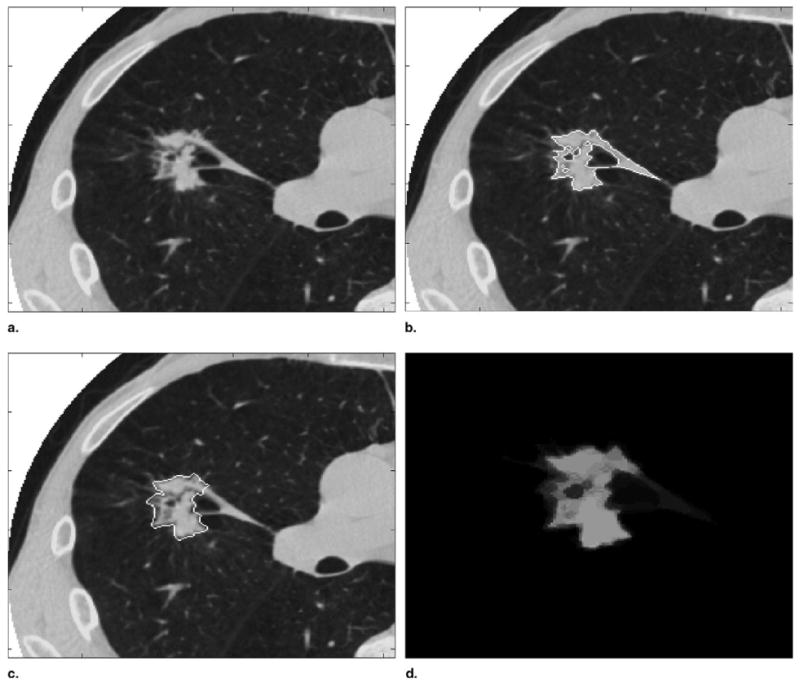
(a) Nodule 10, slice 20. (b) Radiologist 6, method 2 edge map. (c) Radiologist 4, method 3 edge map. (d) p-map computed by summing all radiologist-method mask combinations.

Much like jack-knifing, the edge to be tested should not contribute to the combined p-map because doing so increases the correlation between the edge under test with the p-map values and thus decreases the sensitivity of the test. A radiologist-method combination was excluded from the combined p-map by subtracting it from the combined sum of edge masks, normalizing by the denominator of n – 1, spatial filtering, and transforming the resulting sampled p-map values. The same process was applied to all slices containing any nodule annotation.

The sparse sampling of the edge map for each combination of radiologist-method occurred at random multiples of 10 voxels along edge maps on each MDCT slice to assure decorrelation of the previously smoothed p-map samples (Fig 2). Sampling too sparsely should be avoided because it reduces the number of samples for each nodule and thus reduces the power of the statistical test for significant differences. As each sampled p-map value was appended to the p-map vector to construct the dependent variable used in the statistical test, the corresponding method and radiologist vectors (ie, the independent variables) were simultaneously created. Entries for the radiologists and methods vectors consisted of values 1–6 and 1–3, respectively, corresponding to the radiologist-method combination that generated the particular p-map sample. Last, because probability values tend not to be Gaussian distributed, the sampled p-map values were transformed to obtain a nearly Gaussian distribution as visualized by the normal probability plot seen in Fig 3. The typical transformation, and that applied here, to normalize probability values is

Figure 2.

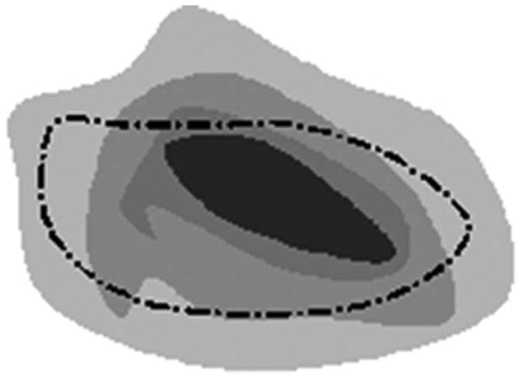
Dashed line shows contour from one radiologist-method combination. Dots depict loci of possible samples from the underlying p-map constructed from the sum of other radiologist-method combinations.

Figure 3.

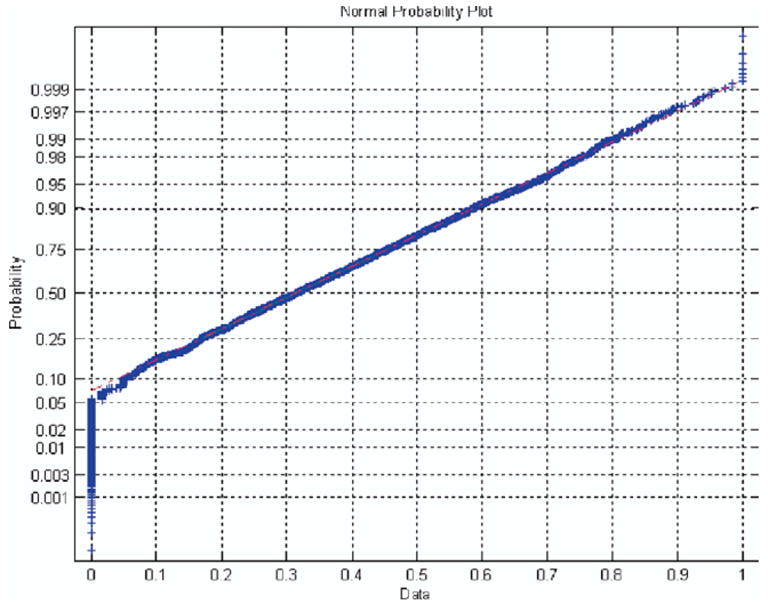
Normplot of all transformed, smoothed, sampled p-map values for all radiologist-method combinations across all nodules.

$$y=arcsin(sqrt(p))/(\pi /2)$$

where y is the new transformed variable plotted in Fig 3 and that used in the statistical test and p is the originally sampled, smoothed p-map value. A Gaussian distributed variable would yield a straight line in the normplot of Fig 3. The null hypothesis assumes that the variability of the p-map values sampled under the edge maps of each radiologist-method combination is unbiased (ie, randomly unrelated to radiologist or method).

p-map Model

Several linear mixed effect models were fitted to the p-map data. The lme function in the R (21) package nlme (22) was used to perform the statistical analysis using the method of maximum likelihood. Model selection was performed using the Bayesian information criteria (23). The final model included main radiologist and method effects as well as interactions between radiologists and methods. Random effects included a random nodule effect, a random radiologist effect nested within nodule, and a random method effect nested with radiologist and nodule. These random effects help account for the correlation between p-map values that were constructed for each nodule by a single radiologist under each of the three methods.

The use of the linear mixed-effects model, specifically lme as described previously, is preferable to typical analysis of variance (ANOVA) methods, because use of the typical multiple comparison methods and corrections for multiple observations that follow ANOVA are not necessary; instead by using lme, individual parameter estimates are computed directly from the data. It is worth noting that the general trends in the results computed by lme for our data sets are similar to those computed by ANOVA, but the individual parameter values are biased in ANOVA because of the lack of ability to handle nested, random effects.

For the lme, let Y^hijk denote the hth transformed p-map value from radiologist i, method j, nodule k. The final model is

$$Y_{\mathit{hijk}}=\alpha +a_k+{\beta }_i^R+b_{i(k)}+{\beta }_j^M+c_{j(ik)}+{\beta }_{ij}^{RM}+{\epsilon }_{\mathit{hijk}}$$

where α is the model intercept, ${\beta }_i^R$ is the main radiologist effect, ${\beta }_j^M$ is the main method effect, ${\beta }_{ij}^{RM}$ is the interaction term between radiologist and method, α_k is the random nodule effect, b_i(k) is the random radiologist effect within nodule, c_j(ik) is the random method effect within radiologist and nodule, and ε_hijk is the model error. Each random effect is assumed to have a mean zero normal distribution, as is the error term. The random effects are also assumed to be uncorrelated with each other. For example, the correlation between α_k and a_k*, k ≠k*, equals zero as well as between b_i(k) and c_j(ik) for all i,j,k. Parameter estimates and P values are given in Table 1.

Table 1.

lme Results of Parameter Estimates for p-map Values

Parameter	Estimate	Standard Error	DF	t Value	P Value
α	0.1518	0.0195	9469	7.7682	<.0001
${\beta }_2^R$	0.3117	0.0289	110	10.7798	<.0001
${\beta }_3^R$	0.0822	0.0278	110	2.9614	.0038
${\beta }_4^R$	0.1943	0.0283	110	6.8644	<.0001
${\beta }_5^R$	0.2679	0.0289	110	9.2645	<.0001
${\beta }_6^R$	0.1833	0.0286	110	6.4173	<.0001
${\beta }_2^M$	0.1892	0.0260	261	7.2720	<.0001
${\beta }_3^M$	0.1067	0.0258	261	4.1364	<.0001
${\beta }_{22}^{RM}$	−0.2294	0.0381	261	−6.0246	<.0001
${\beta }_{32}^{RM}$	−0.1105	0.0367	261	−3.0143	.0028
${\beta }_{42}^{RM}$	−0.2460	0.0371	261	−6.6351	< .0001
${\beta }_{52}^{RM}$	−0.1842	0.0381	261	−4.8399	< .0001
${\beta }_{62}^{RM}$	−0.0233	0.0387	261	−0.6008	.5485
${\beta }_{23}^{RM}$	−0.2871	0.0377	261	−7.6056	< .0001
${\beta }_{33}^{RM}$	−0.1427	0.0363	261	−3.9300	.0001
${\beta }_{43}^{RM}$	−0.2012	0.0369	261	−5.4485	< .0001
${\beta }_{53}^{RM}$	−0.1710	0.0382	261	−4.4750	< .0001
${\beta }_{63}^{RM}$	−0.1493	0.0373	261	−4.0039	.0001

Volume Model

Several linear mixed-effect models were fitted to the natural log-transformed volume data. The log transform of the nodule volume data was required to yield Gaussian Pearson residuals. The lme function in the R package nlme was used to perform the statistical analysis using the method of maximum likelihood. Model selection was performed using the Bayesian information criteria. The final model included main radiologist and method effects as well as interactions between radiologists and methods. Random effects included a random nodule effect and a random radiologist effect nested within nodule. The random effects help account for the correlation induced between volumes of a single nodule constructed by a radiologist under the three different methods.

Let Y_ijk denote the log volume from radiologist i, method j, nodule k. The final model is

$$Y_{\mathit{ijk}}=\alpha +a_k+{\beta }_i^R+b_{i(k)}+{\beta }_j^M+c_{j(ik)}+{\beta }_{ij}^{RM}+{\epsilon }_{\mathit{ijk}}$$

where α is the model intercept, ${\beta }_i^R$ is the main radiologist effect, ${\beta }_j^M$ is the main method effect, ${\beta }_{ij}^{RM}$ is the interaction term between radiologist and method, α_k is the random nodule effect, b_i(k) is the random radiologist effect with nodule, c_j(ik) is the random method effect within radiologist, and nodule and ε_ijk is the model error. Each random effect is assumed to have a mean zero normal distribution, as is the error term. The random effects are also assumed to be uncorrelated with each other and with the model error. For example, the correlation between α_k and a_k*, k ≠k*, equals zero as well as between b_i(k) and c_j(ik) for all i,j,k. Parameter estimates and P values are tabulated in Table 2.

Table 2.

lme Results of Parameter Estimates for Nodule Volumes

Parameter	Estimate	Standard Error	DF	t Value	P Value
α	6.7853	0.3608	264	18.8038	< 0.0001
${\beta }_2^R$	−1.0613	0.1257	110	−8.4440	< .0001
${\beta }_3^R$	−0.2529	0.1257	110	−2.0123	.0466
${\beta }_4^R$	−0.6922	0.1257	110	−5.5076	< .0001
${\beta }_5^R$	−1.0383	0.1257	110	−8.2614	< .0001
${\beta }_6^R$	−0.7654	0.1257	110	−6.0895	<.0001
${\beta }_2^M$	−0.6244	0.1104	264	−5.6542	<.0001
${\beta }_3^M$	−0.3459	0.1104	264	−3.1324	.0019
${\beta }_{22}^{RM}$	0.7765	0.1562	264	4.9724	<.0001
${\beta }_{32}^{RM}$	0.3629	0.1562	264	2.3241	.0209
${\beta }_{42}^{RM}$	0.8443	0.1562	264	5.4065	<.0001
${\beta }_{52}^{RM}$	0.7147	0.1562	264	4.5763	<.0001
${\beta }_{62}^{RM}$	0.0150	0.1562	264	0.0963	.9234
${\beta }_{23}^{RM}$	0.9527	0.1562	264	6.1004	<.0001
${\beta }_{33}^{RM}$	0.4866	0.1562	264	3.1162	.0020
${\beta }_{43}^{RM}$	0.7104	0.1562	264	4.5491	<.0001
${\beta }_{53}^{RM}$	0.5997	0.1562	264	3.8405	.0002
${\beta }_{63}^{RM}$	0.6857	0.1562	264	4.3907	<.0001

RESULTS

For the parameter estimates of the nodule p-map model in Table 1, note that only one term (ie, the interaction term between radiologist 6 and method 2) is not significantly different from zero at P < .05. Further analysis of the sum of squares attributed to each variable category leads to the following summary of the model’s resolution of signal and noise shown in Table 3 across all nodules. Also note from Table 3 that the radiologists’ term accounts for four times the variance compared with that of the method term, and that random error accounts for 60% of the total variance.

Table 3.

Summary of lme p-map Model’s Sum of Squares for Each of the Modeled Categories

p-map Model	Sum of Squares	% Variance Explained
Intercept	83.633	20.69
Radiologist	60.746	15.03
Method	13.927	3.45
Interaction	2.65	0.66
Error	243.234	60.18
Total	404.19

Additionally the p-map lme results were used to compute individual estimates of each of the radiologist-method combination performances as shown in Fig 4.

Figure 4.

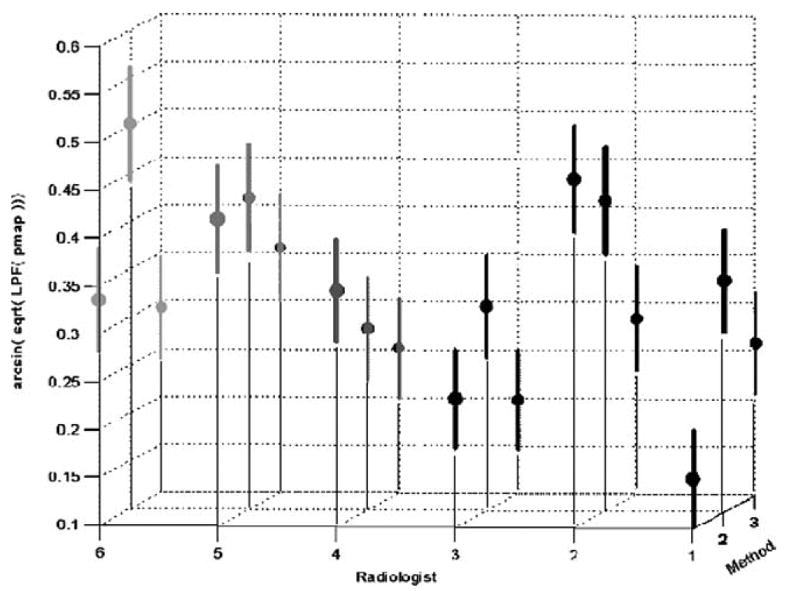
Radiologist-method combinations for the transformed, low-pass filtered, p-map data (means and 99% confidence regions are indicated).

Typically, results for data collected by an experiment such as this would be presented only as a volumetric nodule analysis. Because characterization of nodules often depends on boundary descriptions, we present both a volume analysis, which follows, and a p-map analysis, already demonstrated, that compares the individual localized radiologist-method tracing positions. Clearly, because p-maps, as well as their transform used here, have values approaching unity near the center of the nodule and approaching zero peripherally, we should expect to see negative correlations between volume data and p-map data. More specifically, radiologist-method combinations that tend to have higher p-map values are drawn more centrally and thus tend to yield smaller volume estimates.

For the parameter estimates of the nodule volume model, note that only one term (ie, the interaction term between radiologist 6 and method 2 and the same as seen in the p-map results) is not significant at P < .05. Further analysis of the sum of squares attributed to each variable category leads to the following summary of the model’s resolution of signal and noise shown in Table 4 across all nodules. Note that for the volume model, the resulting random error is only 11% of the total, and that the variances explained by radiologist and method differ by a factor of 130%, smaller than the 400% obtained from the p-map results.

Table 4.

Summary of lme Volume Model’s Sum of Squares for Each of the Modeled Categories

Volume Model	Sum of Squares	% Variance Explained
Intercept	41.51	13.26
Radiologist	126.491	40.42
Method	97.218	31.06
Interaction	97.218	3.95
Error	35.409	11.31
Total	312.976

Similarly the volume lme results were used to compute individual estimates of each of the radiologist-method combination performances as shown in Fig 5. The vertical axis was chosen to be the negative of the log volume to allow easy visual verification of the strong negative correlation between trends in results of the p-map and volume models.

Figure 5.

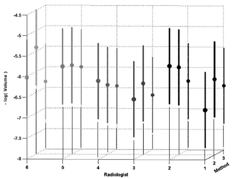
Radiologist-method combinations for negative log-transformed volume data (means and 99% confidence regions are indicated).

By looking across the volumes of all radiologist-method combinations for all nodules, we observed that the regression of the log of standard deviation appears to be linear with the log of the mean and that the random errors of the regression fit appear to be drawn from the same distribution independent of mean. Indeed, for this fit, we obtain the correlation coefficient r² = .922 at α < 10⁻⁴. Figure 6 shows a linear fit of the nodule volumes’ standard deviation vs. mean on a log-log plot. When plotted on a linear graph, the corresponding line in Fig 7 is also nearly linear. Such a plot suggests that the standard deviation (ie, the standard error of the volume estimates) is approximately a fixed percentage of the volume where the percentage is represented by the slope of the curve (ie, approximately 20%). Others have shown similar linear relationships between mean size and standard deviation (20).

Figure 6.

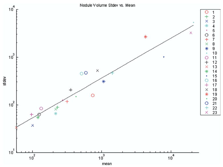
Log-log plot of standard deviation vs. mean for volumes in pixels across all nodules (nodule number is indicated in legend).

Figure 7.

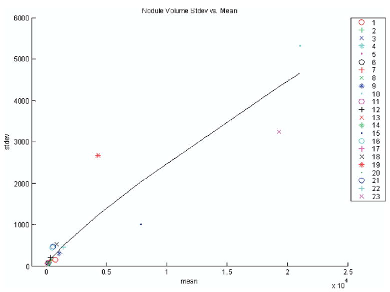
Plot of standard deviation vs. mean for volumes in pixels across all nodules on linear axes.

DISCUSSION

P-maps

All of the coefficients of the linear mixed-effects model shown in Table 1 derived from p-map values are statistically different from zero at P < .05 except one interaction term. Although the modeled variance for radiologists was more than four times that of methods, by far the largest variance, almost 60% and four times larger than that of the radiologists, was due to random error. The magnitude of the residual error for the p-map analysis accentuates the point that segmentation is fundamentally a noisy task independent of reader and method. Because this task did not involve repeated measures, it is impossible to verify whether a single radiologist-method combination would have similar random variance.

From Fig 4, note that four radiologist-method combinations (ie, 1–2, 4–1, 5–3, and 6–1) all share a role as seeds for the largest cluster of 13 not significantly different radiologist-method combinations at P = .01 as indicated in Table 5; the remaining radiologist-nodule combinations are indeed significantly different from these seeds at P = .01.

Table 5.

X’s Mark the Largest p-map Cluster of 13 Not Significantly Different Radiologist-Method Combinations at P = .01 (Gray Cells Represent Radiologist’s Method of Choice)

	Radiologist
Methods	1	2	3	4	5	6
1				x	x	x
2	x	x	x	x	x
3	x	x		x	x	x

Volumes

All of the coefficients of the linear mixed-effects model shown in Table 2 derived from volumes are statistically significant at P < .05 except one interaction term. Although from Fig 5 we see that the trends in the negative log volume closely mimic those seen in the p-map results of Fig 4, none of the radiologist-method combinations is significantly different. Additionally, we observe that the resulting random volume error after modeling is a much smaller percentage (ie, 11%) of the total variance than that obtained from the p-map analysis. Recall that volume estimation is fundamentally an integrative process where errors in individual edge map positions sum to a small, if not zero, volume contribution.

From Fig 7 we see that the standard error of nodule volume estimates across all radiologist-method combinations is approximately 20% of the volume. The presence of this proportionality is described by a gamma distribution. To put this into perspective, note that the 95% confidence region extends over the huge range from 64% to 143% of the mean nodule volume. Because variances add, using manual or semiautomatic segmentation to detect the volume change of a nodule from the difference of two segmented interval examinations will on average have an approximate maximum standard error of 0.20 √2 = 0.28, or approximately 28% of the nodule’s (mean) volume. Hence we derive that the measured nodule volume would have to increase/decrease by more than 55% of the nodule’s volume to have at least 95% confidence that the measured difference represents a real volumetric change instead of random measurement noise. Because these data were accumulated across methods and radiologists, and typically volume change analysis would be performed using the same radiologist-method combination, these limits can be thought of as upper bounds on lesion volume change estimation error. Even so, Fig 7 and the derived upper bounds have direct implications for the National Cancer Institute–sponsored RIDER project, where the effort is to construct a reference image database to evaluate the response (RIDER) of lung nodules to therapy. Clearly identifying a low noise method of estimating nodule volume change is important. Thus the use of data-sets containing real nodules that remain stable between interval examinations is vitally important in evaluating the noise of nodule volume change assessment methods.

Comparison of p-map and Volumetric Methods

From observation of Fig 4 and 5 and Tables 2 and 4, we conclude that although the analysis of p-map results in a larger fractional modeling error, clearly the statistical power of the p-map analysis is greater than that of the volumetric analysis, which results in larger fractional confidence intervals to the extent that no significant differences can be seen between radiologist-method combinations. In the more sensitive and specific p-map analysis the variance from radiologists vs. methods is large (ie, a factor of 4 times, whereas in the volume analysis the variance ratio is only 1.3). We potentially explain the large difference in the resulting residual error terms between the two measurement analyses by observing that the p-map measurement process is sensitive to central-peripheral position wanderings of the tracings during segmentation, whereas the volume measurement essentially integrates all of the central-peripheral wanderings and thus is less noisy and less sensitive to differences. The increased statistical power of the p-map is a further reason for including these data in the publicly available LIDC data set.

Additionally, we observe that the largest source of variation between radiologists and methods in either analysis rests with the radiologists. Thus even with allowing radiologists to choose their favorite method of nodule annotation, only one radiologist’s method of choice lies slightly outside the cluster of 13 not significantly different combinations at P = .01, as shown in Table 5. This is an important observation in that radiologists can choose any of the three supporting annotation methods tested without adding much in the way of significant variance to the resulting LIDC database. Finally, we note that the median outline described from all the radiologist-method combinations appears by visual inspection to be a good segmentation of each of the lesions.

References

- 1.USPH Service. Smoking and health: report of the Advisory Committee to the Surgeon General of the Public Health Service. Washington, DC: Government Printing Office; 1964. [Google Scholar]
- 2.Valdespino VM, Valdexpino VE. Cervical cancer screening: state of the art. Curr Opin Obstet Gynecol. 2006;18:35–40. doi: 10.1097/01.gco.0000192971.59943.89. [DOI] [PubMed] [Google Scholar]
- 3.Herbst R, Bajorin D, Bleiberg H, et al. Clinical cancer advances 2005: major research advances in cancer treatment, prevention, and screening—a report from the American Society of Clinical Oncology. J Clin Oncol. 2006;24:190. doi: 10.1200/JCO.2005.04.8678. [DOI] [PubMed] [Google Scholar]
- 4.Fontana RS, Sanderson DR, Woolner LB, et al. Lung cancer screening: the Mayo program. J Occup Med. 1986;28:746–750. doi: 10.1097/00043764-198608000-00038. [DOI] [PubMed] [Google Scholar]
- 5.Truong M, Munden R. Lung cancer screening. Curr Oncol Rep. 2003;5:309–312. doi: 10.1007/s11912-003-0072-0. [DOI] [PubMed] [Google Scholar]
- 6.Henschke CI, Miettinen O, Yankelevitz D, et al. Radiographic screening for cancer. Clin Imaging. 1994;18:16–20. doi: 10.1016/0899-7071(94)90140-6. [DOI] [PubMed] [Google Scholar]
- 7.Henschke CI, McCauley D, Yankelevitz D, et al. Early Lung Cancer Action Project: overall design and findings from baseline screening. Lancet. 1999;354:99–105. doi: 10.1016/S0140-6736(99)06093-6. [DOI] [PubMed] [Google Scholar]
- 8.Henschke CI, Yankelevitz D, Libby D, et al. CT screening for lung cancer: the first ten years. Cancer J. 2002;8:54. [PubMed] [Google Scholar]
- 9.Henschke CI, Yankelevitz D, Kostis W. CT screening for lung cancer. Semin Ultrasound CT MR. 2003;24:23–32. doi: 10.1016/s0887-2171(03)90022-9. [DOI] [PubMed] [Google Scholar]
- 10.Aberle D, Gamsu G, Henschke C, et al. A consensus statement of the Society of Thoracic Radiology: screening for lung cancer with helical computed tomography. J Thorac Imaging. 2001;16:65–68. doi: 10.1097/00005382-200101000-00010. [DOI] [PubMed] [Google Scholar]
- 11.Swensen SJ, Jett JR, Hartman TE, et al. Lung cancer screening with CT: Mayo clinic experience. Radiology. 2003;226:756–761. doi: 10.1148/radiol.2263020036. [DOI] [PubMed] [Google Scholar]
- 12.Recruitment begins for lung cancer screening trial. J Natl Cancer Inst. 2002;94:1603. [PubMed] [Google Scholar]
- 13.Armato SG, McLennan G, McNitt-Gray MF, et al. The Lung Image Database Consortium: developing a resource for the medical imaging research community. Radiology. 2004;232:739–748. doi: 10.1148/radiol.2323032035. [DOI] [PubMed] [Google Scholar]
- 14.Clarke L, Croft B, Staab E, et al. National Cancer Institute initiative: lung image database resource for imaging research. Acad Radiol. 2001;8:447–450. doi: 10.1016/S1076-6332(03)80555-X. [DOI] [PubMed] [Google Scholar]
- 15.Dodd LE, Wagner RF, Armato SG, et al. Assessment methodologies and statistical issues for computer-aided diagnosis of lung nodules in computed tomography: contemporary research topics relevant to the Lung Image Database Consortium. Acad Radiol. 2004;11:462–475. doi: 10.1016/s1076-6332(03)00814-6. [DOI] [PubMed] [Google Scholar]
- 16.Bobot N, Kazerooni E, Kelly A, et al. Inter-observer and intra-observer variability in the assessment of pulmonary nodule size on CT using film and computer display methods. Acad Radiol. 2005;12:948–956. doi: 10.1016/j.acra.2005.04.009. [DOI] [PubMed] [Google Scholar]
- 17.Erasmus JJ, Gladish GW, Broemeling L, et al. Interobserver and intraobserver variability in measurement of non-small-cell carcinoma lung lesions: implications for assessment of tumor response. J Clin Oncol. 2003;21:2574–2582. doi: 10.1200/JCO.2003.01.144. [DOI] [PubMed] [Google Scholar]
- 18.Schwartz LH, Ginsberg MS, DeCorato D, et al. Evaluation of tumor measurements in oncology: use of film-based and electronic techniques. J Clin Oncol. 2000;18:2179–2184. doi: 10.1200/JCO.2000.18.10.2179. [DOI] [PubMed] [Google Scholar]
- 19.Tran LN, Brown MS, Goldin JG, et al. Comparison of treatment response classifications between unidimensional, bidimensional, and volumetric measurements of metastatic lung lesions on chest computed tomography. Acad Radiol. 2004;11:1355–1360. doi: 10.1016/j.acra.2004.09.004. [DOI] [PubMed] [Google Scholar]
- 20.Judy PF, Koelblinger C, Stuermer C, et al. Reliability of size measurements of patient and phantom nodules on low-dose CT, lung-cancer screening. Radiology. 2002;225(Suppl S):497–497. [Google Scholar]
- 21.Team RDC. R: a language and environment for statistical computing. Vienna, Austria: R Foundation for Statistical Computing; 2005. [Google Scholar]
- 22.Pinheiro J, Bates D, DebRoy S, et al. nlme: linear and nonlinear mixed effects models. R package version 3.1–60. [Accessed August 8, 2006]; Available online at: http://www.cran.r-project.org/src/contrib/Descriptions/nlme.html.
- 23.Schwarz G. Estimating the dimension of a model. Ann Statistics. 1978;6:461–464. [Google Scholar]