Using prior knowledge in the determination of macromolecular size distributions by analytical ultracentrifugation

Abstract

Analytical ultracentrifugation has reemerged as a widely used tool for the study of ensembles of biological macromolecules to understand, for example, their size-distribution and interactions in free solution. Such information can be obtained from the mathematical analysis of the concentration and signal gradients across the solution column and their evolution in time generated as a result of the gravitational force. In sedimentation velocity analytical ultracentrifugation, this analysis is frequently conducted using high resolution, diffusion-deconvoluted sedimentation coefficient distributions. They are based on Fredholm integral equations, which are ill-posed unless stabilized by regularization. In many fields, maximum entropy and Tikhonov-Phillips regularization are well-established and powerful approaches that calculate the most parsimonious distribution consistent with the data and prior knowledge, in accordance with Occam’s razor. In the implementations available in analytical ultracentrifugation, to date, the basic assumption implied is that all sedimentation coefficients are equally likely, and that the information retrieved should be condensed to the least amount possible. Frequently, however, more detailed distributions would be warranted by specific detailed prior knowledge on the macromolecular ensemble under study, such as, the expectation of the sample to be monodisperse or paucidisperse, or the expectation for the migration to establish a bimodal sedimentation pattern based on Gilbert & Jenkins’ theory for the migration of chemically reacting systems. So far, such prior knowledge has remained largely unused in the calculation of the sedimentation coefficient or molecular weight distributions, or was only applied as constraints. In the present paper, we examine how prior expectations can be built directly into the computational data analysis, conservatively in a way that honors the complete information of the experimental data, whether or not consistent with the prior expectation. Consistent with analogous results in other fields, we find that use of available prior knowledge can have a dramatic effect on the resulting molecular weight, sedimentation coefficient and size-and-shape distributions, and significantly increase both their sensitivity and resolution. Further, the use of multiple alternative priors allows to probe the range of possible interpretations consistent with the data.

INTRODUCTION

Analytical ultracentrifugation is a classical first-principle technique for the characterization of biological macromolecules, widely used in the studies of proteins ^1–3, carbohydrates ^4–6, nucleic acids ^7,8, as well as man-made macromolecules, including polymers ⁹, compounds in supramolecular chemistry ^10,11, drug delivery particles ¹², and others ^13–15. Due to improved instrumentation and data analysis approaches it has experienced a renaissance ¹⁶, in particular for the characterization of reversible macromolecular self- and hetero-association processes. Analytical ultracentrifugation is uniquely suited to determine the number, size, and gross shape and conformation of non-reversible and reversible macromolecular complexes, study their interaction with ligands, and observe the assembly of multi-protein complexes. In particular, sedimentation velocity analytical ultracentrifugation (SV), which is concerned with the time-course of migration of the macromolecular ensemble in the gravitational field, provides a combination of strongly size-dependent migrations that leaves the faster sedimenting protein complexes always in a bath of the slower sedimenting macromolecular components. Such a situation allows reversibly assembled complexes to be maintained throughout the experiment, and their migration to be observed in a way that quantitatively reflects the equilibrium and kinetic properties of the interaction.

SV has been transformed by the application of modern data analysis approaches that globally fit the raw sedimentation data directly with the partial differential equation for single or multi-component sedimentation ^17–27. Frequently, the ensemble of sedimenting macromolecules is described by a sedimentation coefficient distribution. This can account for heterogeneity and for trace populations in the macromolecular sample, and due to the exquisite sensitivity of SV, is frequently required in order to achieve a satisfactory fit to the data and avoid misinterpretation of the boundary spread. Sedimentation coefficient distributions, and more general size-and-shape distributions, permit the interpretation of both the translation and the evolution of the shape of the sedimentation boundary, providing estimates for sedimentation coefficients, molar mass, and heterogeneity of the macromolecular sample under study ^21,27–29. For example, a hydrodynamic scaling law can be used to extract a measure for the average degree of size-dependent diffusion from the shape of the sedimentation boundary, resulting in diffusion-deconvoluted sedimentation coefficient distributions, termed c(s) ^21,28. Many applications have taken advantage of the high resolution of this method ³⁰, its high sensitivity for the quantitation of trace components ^31–33, and its more recent extensions to multi-signal analysis of multi-component sedimentation processes ^34–37.

Mathematically, the decomposition of the experimental data in terms of signals from an unknown number of species sedimenting with different rates requires the inversion of a Fredholm integral equation. Such problems are common to many imaging disciplines and many experimental biophysical techniques, and their properties have been well-studied ³⁸. They are ill-posed and have the common characteristics that usually many different solutions fit the data equally well within the noise of the experimental data. Commonly, details of the experimental noise can be amplified and lead to dominant features in the calculated distributions ^39,40. Although SV has very rich data sets (typically consisting of 10⁴–10⁵ data points with signal-to-noise ratio between 10² and 10³), and the signals from size-dependent migration allow for easier discrimination than the exponential signals encountered in many other biophysical techniques, this is still the major limitation in the resolution and sensitivity that can be achieved in the study of macromolecular sedimentation by SV.

To our knowledge, Stephen Provencher’s computer program CONTIN was the first to introduce the regularization approach into the biophysical analysis ^39–41. Regularization is the introduction of a bias to select, among all possible statistically indistinguishable solutions, the one that conforms best with a predefined property. It can be understood as a constrained optimization that selects the most parsimonious distribution among all distributions that fit the raw data statistically indistinguishably well. This selection can be justified by Occam’s razor, and in countless applications in many different disciplines regularization it has proven to be a remarkably powerful approach. In the field of SV, it has been implemented in the programs SEDFIT and SEDPHAT, using maximum entropy (ME) ^42,43 and Tikhonov-Phillips (TP) ^44,45 regularization.

The ME principle can be understood in the more general framework of Bayesian statistics, in which data are interpreted in light of existing prior probabilities ^46,47. Similarly, methods have been established for incorporating prior expectation in the generalized TP regularization ^48–50. It is well established in modeling that, generally, the use of prior information can substantially enhance the ability to extract information from experimental data ^47,51. Therefore, instead of selecting simply the most parsimonious distribution from all that fit the data indistinguishably well, prior probabilities allow a better choice by selecting the distribution that is most consistent with existing a priori knowledge. Accordingly, the use of prior information is currently exploited in a wide range of fields to improve the inversion of Fredholm integral equations.

Nevertheless, so far in the implementation of regularization for SV, only the simplest regularization approach was utilized, always assigning equal a priori probability to the likelihood of all sedimentation coefficients to generate the most parsimonious distribution, and in this way considering solely information residing in the data to be analyzed. Although this is conservative and many applications have shown it to be a very robust approach, it has several drawbacks. For example, the peak widths obtained depend on the signal-to-noise ratio of the data acquisition and the number of significant data points available, which makes them not easily interpretable ⁵². Further, it does not take advantage of a wealth of specific knowledge that is frequently available about the macromolecular ensemble under study. Such knowledge can be derived from expectations based on hydrodynamic scaling laws, from sedimentation data acquired with different detection systems, and/or from characterizing separately different components of a multi-component mixture under study.

In a hierarchical approach, some of this knowledge has been incorporated into a secondary analysis in the form of a fixed constraint (for example, with the hybrid discrete/continuous distribution ^29,53–55), in combination of statistical analysis of the quality of fits obtained. However, in the present work we examined a more subtle approach, which permits the experimental data to override our expectation if they contain sufficient information contrary to our expectation. This can be naturally achieved in the framework of incorporating prior expectations directly into the computed molecular weight distribution c(M) from SE, and sedimentation coefficient distributions c(s) or the size-and-shape distributions c(s,f_r) and their equivalents from SV. In the following, we will describe in theory and practice the incorporation of different forms of prior expectation applied to the analysis of different macromolecular systems, and explore the relationship between the information content of the data and (correct or impostor) prior expectation as determinants of the computed distributions. We found that the incorporation of prior knowledge can have a profound influence on the sedimentation coefficient distributions, and can frequently aid in obtaining more information from the experimental data. Dependent on the prior knowledge used, it can lead to greatly improved resolution, for example, for discriminating macromolecular complexes in solution or for examining micro-heterogeneity in size and/or conformation, and it can provide enhanced sensitivity and quantitation of trace components. This tool is implemented in the public domain software SEDFIT ⁵⁶.

METHODS

Analytical Ultracentrifugation

Sedimentation velocity experiments were conducted as described in the experimental protocol ⁵⁷. Briefly, 400 μl samples of dilute protein solutions were loaded in the sample sector of Epon double-sector centerpieces and buffer was loaded in the reference sector. For details on the sample preparation, see 34. The centrifugal cell assembly was inserted in an An50 Ti eight-hole rotor and temperature equilibrated for approximately one hour at 20°C at rest in the chamber of an Optima XLI (Beckman Coulter, Fullerton, CA). After rotor acceleration to 50,000 rpm, the evolution of radial concentration profiles was observed in real-time with the absorbance and/or interference optical system. Series of scans comprising the entire sedimentation process were loaded in the software SEDFIT ⁵⁶, and modeled over the entire time and radial range (excluding the regions of optical artifacts and of back-diffusion) as described below, treating the exact meniscus position as an unknown parameter. Systematic time-invariant and radial-invariant noise contributions were determined by algebraic noise decomposition based in least-squares optimization ²⁰.

Calculating Sedimentation Coefficient Distributions c(s)

Sedimentation coefficient distributions c(s) were determined by numerical inversion of the Fredholm integral equation

$$a(r,t)\cong \int c(s){\chi }_1(s,D(s),r,t)ds$$ (1)

^21,28 where a(r,t) denotes the experimentally measured signal, χ₁(s,D,r,t) denotes the normalized solution to the Lamm equation for a single species

$$\frac{\partial \chi }{\partial t}+\frac{1}{r}\frac{\partial }{\partial r}\left[r\left(s{\omega }^{2}r\chi -D\frac{\partial \chi }{\partial r}\right)\right]=0$$ (2)

⁵⁸ using the symbol χ(r,t) for the macromolecular concentration distribution as a function of radial position and time, ω for the rotor angular velocity, and s and D for the macromolecular sedimentation and diffusion coefficient, respectively. Modifications of Eq. 2 to account for pressure effects from solvent compressibility and dynamic density gradients from sedimenting co-solvents have been described ^59,60, and can be inserted into the integral equations without affecting the applicability of the regularization strategy discussed in the present paper. Obviously, we request that c(s) is positive throughout. The relationship between D and s was approximated with the hydrodynamic scaling law

$$D(s)=\frac{\sqrt{2}}{18\pi }kT\hspace{0.17em}{s}^{-1/2}{\left(\eta {(f/f_0)}_w\right)}^{-3/2}{\left((1-\overline{v}\rho )/\overline{v}\right)}^{1/2}$$ (3)

where k denotes the Boltzmann constant, T the absolute temperature, v̄ the protein partial specific volume, and ρ and η the solvent density and viscosity. It is based on a weight-average frictional ratio (f/f₀)_w of all sedimenting species. Other scale relationships are possible and have been implemented in SEDFIT, for example, for worm-like chains, for bimodal distributions with heterogeneous frictional coefficient, and for empirically user-defined relationships. Although the sedimentation coefficient distribution c(s) is based on a linear combination of Lamm equation solutions of non-interacting species, it was shown that it is applicable also to systems of rapidly interacting macromolecules. In this case, c(s) reports approximations of the asymptotic reaction boundary at infinite time described in Gilbert-Jenkins theory ⁶¹, i.e. transport properties of the coupled reacting system rather than the properties of the interacting species ⁶². Eq. 2 was solved for each pair of s- and D-values using finite element solutions as described in (Brown, P., and Schuck, P., A new adaptive grid-size algorithm for the efficient and accurate simulation of sedimentation velocity profiles, manuscript submitted).

Calculating Size-And-Shape Distributions c(s,M) and General Sedimentation Coefficient Distributions c(s,*)

For cases where the scaling law Eq. 3 is not applicable and no replacement can be identified, or where macromolecular mixtures are studied that are very heterogeneous in hydrodynamic friction and partial-specific volume, a size-and-shape distribution has been defined as

$$a(r,t)=\iint c(s,f_r)\chi (s,D(s,f_r),r,t){\mathit{dsdf}}_r$$ (4)

with the symbol f_r as abbreviation for the frictional ratio f/f₀, and again with c(s,f_r) assuming only positive values. Using the Svedberg relationship, it can be transformed to the equivalent distributions of sedimentation coefficient and molar mass c(s,M), sedimentation coefficient and Stokes radius c(s,R), sedimentation and diffusion coefficient c(s,D), or size and shape c(M,f_r). The inversion of the Fredholm integral equation Eq. 4 is described in ²⁷ and implemented in SEDFIT. It involves similar difficulties as the inversion of Eq. 1, but is slightly more ill-posed due to the typically much lower information content of experimental data on the diffusion dimension.

For cases where the diffusional dimension is not of primary interest, a general sedimentation coefficient distribution was defined as

$$c(s,\ast ):=\int c(s,f_r){df}_r$$ (5)

²⁷. c(s,*) can be considered a more general version of c(s), which does not make any assumptions on the diffusional properties of the macromolecular ensemble, yet still deconvolutes diffusional broadening on the basis of the experimentally measured sedimentation boundary shapes.

Molecular Weight Distributions from Sedimentation Equilibrium

The equilibrium between sedimentation and diffusion attained at long times by a single thermodynamically ideal species follows the Boltzmann exponential

$$c_{\omega }(r,M_{\mathit{buoy}})=\overline{c}\frac{M_{\mathit{buoy}}\left(\xi (b)-\xi (m)\right)}{exp\left(M_{\mathit{buoy}}\xi (b)\right)-exp\left(M_{\mathit{buoy}}\xi (m)\right)}exp\left(M_{\mathit{buoy}}\xi (r)\right)$$ (6)

with M_buoy = M ( 1 − v̄ρ) denoting the buoyant molecular weight, the abbreviation ξ(r)= ω² r²/2RT, the gas constant R, and absolute temperature T ⁶³. This expression describes the redistribution of the macromolecule at initial loading concentration c̄ in a sector-shaped solution column with meniscus m and bottom b. A mixture of macromolecular species produces a signal

$$a_{\omega }(r)=\int \overline{c}(M_{\mathit{buoy}})c_{\omega }(r,M_{\mathit{buoy}})dr\hspace{0.17em}\hspace{0.17em}\hspace{0.17em}\mathit{for}\hspace{0.17em}\mathit{all}\hspace{0.17em}\omega$$ (7)

The index ω indicates that the data will depend on the rotor speed. As described in ⁶⁴, a significantly better estimate for the buoyant molar mass distribution c̄ (M_buoy) can be achieved by globally fitting data sets acquired at different rotor speeds, using the constraints that total mass is conserved (i.e. c̄ is independent of ω).

Regularization With Prior Expectation

The numerical solution of Eq. (1) using maximum entropy (ME) regularization is obtained on a grid of s-values between s_min and s_max (denoted as s_i with i = 1,…,N; N ~ 100 – 300). Accordingly, the discrete form of c(s) consists of a set of values c_i(s_i), which are computed on the basis of the constrained optimization problem

$$\mathit{Min}\left\{\sum _{r,t}{\left(a_{rt}-\sum _i{c}_i{\chi }_{rt}^{(i)}\right)}^2+\alpha \sum _i{c}_{i}log\left(\frac{c_i}{p_i}\right)\right\}$$ (8)

with the indices r and t denoting the radial and time points, ${\chi }_{rt}^{(i)}$ the Lamm equation solution for a species with s_i and D(s_i) at position r and time t. In Eq. 8, the first term represents the least-squares optimization of the fit to the data points a _rt, while the second term represents the ME penalty term with the prior expectation (or short prior) p_i ⁴⁷. The scaling parameter α is iteratively adjusted to a value that ensures that the goodness of fit is not significantly affected by the regularization term, as calculated using Fisher statistics for a pre-determined confidence level (e.g. P = 0.7 for the conventional one standard deviation) ²¹. This follows the strategy previously developed by Provencher in the program CONTIN ^39,41. Due to the large number of data points of an SV experiment (~ 10⁵), the influence of the model parameters c_i on the degrees of freedom is negligible here. For each value of α, Eq. 8 is minimized using the Marquardt-Levenberg method ⁶⁵ implemented with positivity constraints for the c_i.

An alternative regularization approach was developed earlier independently by Tikhonov and Phillips (TP) ^44,45. Here, the penalty term is not the negentropy of the distribution, but a measure for the norm of c(s), implemented in SEDFIT and SEDPHAT as the total curvature ∫(c ″) ² ds. Generalizing this concept, in the presence of prior expectation we minimize the total curvature of the distribution relative to the prior expectation, ∫[(c/p)″]² ds. (This form is motivated by the requirement that in the absence of data, the regularization constraint will produce the expectation, and by the consideration that knowledge of absolute concentrations should not be required). In the discrete form, this leads to a constrained optimization problem analogous to Eq. 8:

$$\mathit{Min}\left\{\sum _{r,t}{\left(a_{rt}-\sum _i{c}_i{\chi }_{rt}^{(i)}\right)}^2+\alpha {\overrightarrow{\mathbf{c}}}^T\mathbf{H}(p)\overrightarrow{\mathbf{c}}\right\}$$ (9)

using the vector notation c⃗ for the 1×N matrix with components c₁,…,c_N. H is a N×N matrix, which in the usual form (without prior expectation) will be identical to the square of the second derivative matrix H^{0 65}. The prior expectation leads to a modification of the matrix elements according to

$$H_{ij}(p)=\frac{H_{ij}^0}{p_i{p}_j}$$ (10)

For the two-dimensional size-and-shape distribution c(s,f_r) [or c(s,M)], as well as for the general c(s,*), the same formalism was used, by extension of the vector notation c⃗ to the concatenated vectors representing components c₁,…,c_N for each f_r-value, forming a 1×N_f×N_s vector, with H⁰ representing the sum of the square of the second derivative matrices in each dimension (with indices chosen accordingly), and the prior expectation p(s,f) similarly discretized in the two-dimensional s-f_r plane.

The conventional sedimentation coefficient distribution obtained with uniform prior probability is termed c(s), while that obtained with specific prior expectations is termed c^(P)(s). For the purpose of the present theoretical study, we identify the distributions with impostor prior expectation as c^(P*⁾(s). In SEDFIT, we implemented the possibility to load an arbitrary distribution from an ASCII file to serve as prior expectations. As tools in selected commonly encountered situations, the following options were implemented:

1. Superpositions of Gaussian distributions at position s_k with user-defined widths σ_k and amplitudes A_k:

   $$p_i=0.001+\sum _k{A}_k{e}^{-{(s_i-s_k)}^2/{\sigma }^2}$$ (11)

   (with 0.001 serving as an arbitrary non-zero reference probability for the remaining distribution) This is motivated by a priori knowledge of s-values of different species.

2. The automatic selection of prior probabilities from an initial analysis with constant p_i. Here, each peak in c(s) of the initial analysis is replaced by a finite grid approximation of a δ-function that has the same weight-average s-value, s_w,k, and area, A_k, of the initial c(s) peak:

   $$p_i=\{\begin{array}{ccc}{p}_l& s_{i^{\ast }}\le s_{w,k}<s_{i^{\ast }+1}& \hspace{0.17em}\\ p_r& s_{j^{\ast }-1}\le s_{w,k}<s_{j^{\ast }}& \mathit{with}\hspace{0.17em}\hspace{0.17em}\hspace{0.17em}{j}^{\ast }=i^{\ast }+1,\\ 0.001& \mathit{else}& \hspace{0.17em}\end{array}$$ (12a)
   where

   $$A_k=0.5p_l(s_{i+1}-s_{i-1})+0.5p_r(s_{j+1}-s_{j-1})$$ (12b)
   and

   $${\int }_{s_{i-1}}^{s_{j+1}}{p}_i{U}_i(s)\mathit{sds}=s_{w,k}{\int }_{s_{i-1}}^{s_{j+1}}{p}_i{U}_i(s)ds$$ (12c)
   with the triangular hat or chapeau functions

   $$U_i(s)=\{\begin{array}{ccc}(s-s_{i-1})/(s_i-s_{i-1})& s_{i-1}\le s\le s_i& \hspace{0.17em}\\ (s_{i+1}-s)/(s_{i+1}-s_i)& s_i<s\le s_{i+1}& \mathit{for}\hspace{0.17em}\hspace{0.17em}\hspace{0.17em}i=2,\dots ,N-1\\ 0& \mathit{else}& \hspace{0.17em}\end{array}$$ (12d)

   spanning the distribution. This leads to a refined analysis accounting for the expectation that the peaks should represent discrete species, which is termed c^(Pδ) in the following.

3. The predictions from Gilbert-Jenkins theory ⁶² for the amplitude and location of the undisturbed component and the shape of the asymptotic reaction boundary component. For example, for a bimolecular heterogeneous interaction of proteins A and B forming a reversible complex AB with mobilities v_A, v_B, and v_C, respectively, the asymptotic boundary profile is given by the equation system

   $$(v-v_a)\frac{\partial m_A}{\partial v}=(v-v_b)\frac{\partial m_B}{\partial v}=-(v-v_c)\frac{\partial m_{AB}}{\partial v}$$ (13)

   which can be solved for each species’ sedimentation coefficient distribution m_A(v), m_B(v), and m_AB(v), in accordance with the mass action law m_Am_B K = m_AB (with the equilibrium association constant K), given each component’s known total concentration ⁶⁶. The complete asymptotic boundary s(v) is given by the sum of each species signal contribution m(v) ⁶¹, and mapped onto the discrete grid to produce the approximation p _i(s_i). The undisturbed boundary component predicted by Eq. 13 is converted into a sharp peak in p_i analogous to Eqs 12.

In this prior probability model, an initial analysis of the sedimentation profiles from a concentration series provides initial estimates for the binding constants and species sedimentation coefficients, which then can be used to refine the division of the sedimentation boundary in the undisturbed and reaction boundary component. This choice of prior probabilities reflects the expected correspondence between the diffusion-deconvoluted sedimentation coefficient distributions c(s) and the asymptotic boundary profile in the absence of diffusion ⁶¹.Footnote 1

All computational methods are implemented in the public domain ultracentrifugal data analysis software SEDFIT ⁵⁶. It can be downloaded from the website, where further supporting and tutorial material will also be made available. Semi-annual tutorial workshops for biophysical data analysis with the software SEDFIT and SEDPHAT are offered at the National Institutes of Health, Bethesda.

RESULTS

Because the analysis of a distribution of exponentials occurs in many different fields and could be regarded as a benchmark for the performance of the modified regularization algorithm, we examine first the effect of prior knowledge on the analysis of sedimentation equilibrium (SE) molecular weight distributions. As an example, we generated synthetic long-column sedimentation equilibria attained by a mixture of three proteins (30 kDa, 50 kDa, and 80 kDa at relative concentrations of 40%, 30%, and 30%, respectively) sequentially at four different rotor speeds, with sedimentation parameters and signal-to-noise ratio as typically encountered in experimental AUC studies ⁵⁷ (inset in Figure 1). The conventional estimate of the molecular weight distribution c(M) without prior knowledge using ME regularization (dotted blue line in Figure 1) results in a bimodal distribution, which demonstrates the well-known lack of resolution and presence of cross-correlation of the Boltzmann exponentials in sedimentation equilibrium. However, we may have knowledge prior to the analysis that species of 30 kDa and 50 kDa should occur, and when the expectation for these two species is implemented by prior probabilities shown as dotted black lines in Figure 1, a trimodal distribution c^(P)(M) (with the superscript ‘(P)’ indicating the incorporation of prior knowledge) is obtained, as shown by the solid green line, which correctly identifies the third species at 80 kDa. Similar results are obtained for both ME and TP regularization. This illustrates that prior knowledge can have a significant effect on the calculated distribution. Similar results were obtained when any combination of two species were known, or when only the middle species was known, but only slight improvement was found when either the smallest or the largest species alone was known (data not shown).

Figure 1.

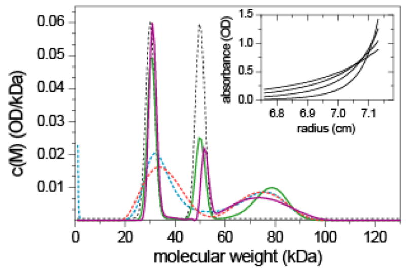
Sedimentation equilibrium analysis with prior knowledge. Sedimentation equilibrium profiles were calculated for a mixture of three proteins with 30 kDa (40%), 50 kDa (30%) and 80 kDa (30%) at sedimentation equilibrium at 10,000 rpm, 12,000 rpm, 15,000 rpm, and 20,000 rpm. A solution column from 6.75 cm to 7.18 cm was assumed, with a total loading signal of 0.5 OD, with 0.01 OD noise of the data acquisition (inset). This mimics the experimental design described in the protocol by Balbo et al ⁵⁷ and the typical experimental signal/noise ratio. Such data may be acquired for a hypothetical mixture of two proteins with 30 kDa and 50 kDa, respectively, forming an irreversible 80 kDa complex. The synthetic data was then analyzed with molecular weight distributions, with regularization scaled to one standard deviation (P = 0.7). In the absence of prior knowledge, the molecular weight distribution c(M) shown as dotted blue and red lines for ME or TP regularization, respectively. If prior knowledge is used about the two protein components used in the mixture, i.e. the knowledge that there may be a 30 kDa species and a 50 kDa species (implemented as Gaussians, black dotted lines), the resulting c^(P)(M) distributions are shown as solid green and purple lines for ME or TP regularization, respectively.

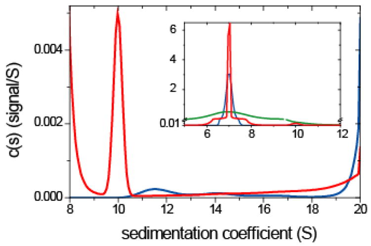
Sedimentation velocity (SV) typically provides a higher resolution than SE, due to the smaller correlation of the signals from macromolecular species of different size. Nevertheless, regularization was also shown to be essential in SV analysis ²¹. In order to demonstrate the effect of prior probabilities on the calculated sedimentation coefficient distribution from SV, we examined the experimental data from a mixture of two similar-sized proteins (Figure 2). We chose a mixture of a preparation of aldolase and IgG (non-reactive to the aldolase), which in individual experiments sedimented at rates of 7.2 S (blue line) and 8.2 S (green line), respectively. When the data from the mixture is analyzed without any regularization, the result is a series of peaks that do not correspond to any of the true sedimenting species (grey line). This is due to the well-known propagation and amplification of experimental noise in Fredholm integral equations ^39,44. The magnitude of this effect depends on the noise level in the data and on the refinement of the discretization of the s-values in the calculated distribution. This makes regularization indispensable for a meaningful analysis. The result of ME regularization with uniform prior, c(s), is shown as the solid black line. This is not using any specific knowledge except requesting the distribution to be parsimonious, and not provide information unless statistically warranted solely by the data to be analyzed. Clearly, this does not enable us to resolve the two species (unless in the context of multi-signal SV, when combined with an additional data signal and information on each protein’s spectral properties ³⁴). We then implemented prior knowledge derived from the s-values of the two proteins observed in their separate sedimentation experiment (dotted red line, showing two Gaussian peaks of height 0.1 at 7.2 and 8.2 S on a background value of 0.001). From the resulting sedimentation coefficient distribution [termed c^(P)(s) in the following] the two species can be readily recognized and resolved (solid red line). This example shows the profound effect that prior expectation can have on the shape of the calculated sedimentation coefficient distribution. We will examine in the following strategies how the interpretation of experimental SV data can be enhanced, and new information generated, when prior knowledge is utilized in the data analysis.

Figure 2.

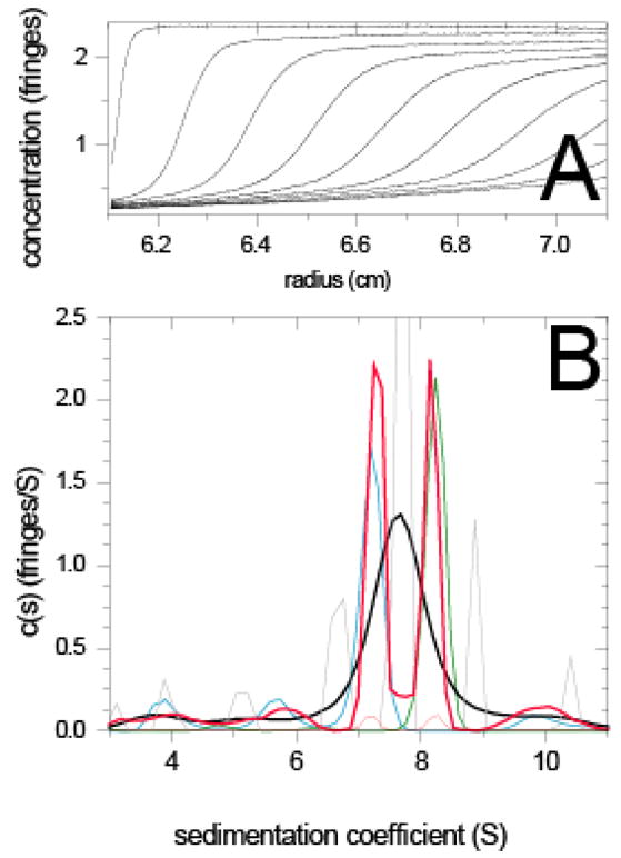
Sedimentation velocity experiment and analysis of a mixture of two similar-sized proteins, IgG1 and aldolase. (A) Concentration gradients of the mixture at different time points during the sedimentation at 50,000 rpm at 26ºC. For experimental details, see 34. (B) Sedimentation coefficient distributions c(s) with ME regularization scaled to one standard deviation (P = 0.7) with uniform prior for the mixture (solid black line) and for the IgG1 and aldolase samples when studied individually in separate experiments at the same concentrations (solid blue and green line, respectively). The c(s) distribution from the mixture without any regularization is shown as grey line exhibiting several peaks. The solid red line is the c^(P)(s) distribution with ME regularization using of prior expectation, with the prior expectation implemented as Gaussians with a width of σ = 0.3 S, centered at the weight-average s-value of the main peak observed in the individual experiments. The peak probabilities are 100fold above the uniform prior in the rest of the distribution (dotted red line).

In order to study in more detail the effect of prior expectation on the resolution, we simulated sedimentation profiles of two species with 7.0 S and 7.1 S, respectively, with normally distributed noise (Figure 3A inset). As a measure of the diffusion-broadened ‘average boundary shape’ in terms of apparent s-values, we calculated the apparent sedimentation coefficient distribution ls-g*(s) (green line) (slightly broader distributions would be obtained from the dc/dt method ⁶⁷). Despite the deconvolution of diffusion in c(s) (black solid line), the two species underlying the simulation cannot be resolved with the standard uniform prior. However, the two species can be correctly distinguished in c^(P)(s) (solid red line) if we make use of the knowledge of the two s-values in the prior probability assignment (dotted red line). On the other hand, the data can be equally well fit with an impostor prior expectation assuming that there be only one single species (blue line). (In the following, this distribution will be termed c^(Pδ*⁾(s), with the superscript ‘P’ to indicate the use of prior knowledge, ‘δ’ to denote the particular prior expectation that there be peaks approximating delta-functions, and ‘*’ to label in the context of the present paper that the prior expectation is impostor.) In this example, since the data do not carry sufficient information on the number and s-values of species within the s-range 7.0 – 7.1 S, the calculated distribution will always reflect the prior probabilities underlying the ME regularization. In fact, species with arbitrarily small differences in s-values may be baseline-resolved (provided appropriate discretization of the range of sedimentation coefficients), and in this sense the resolution is much enhanced, but clearly this does not provide us with new information on the heterogeneity or s-values in the sample. However, this analysis can extract from the data information on the concentration of each of the species (see below).

Figure 3.

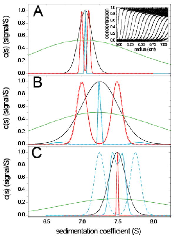
Comparison of sedimentation coefficient distributions obtained using different prior expectations during the analysis of simulated model data. (A) Simulated mixture of two species at equal concentrations sedimenting at 7.0 S and 7.1 S (50,000 rpm, f/f₀ = 1.45, noise = 0.01). Representative concentration distributions at different time-points are shown in the inset. Sedimentation coefficient distributions shown are ls-g*(s) (solid green), c(s) without regularization (grey), and c(s) with standard uniform prior expectations with (solid black, P=0.68). c^(P)(s) distributions with ME regularization are shown with different prior expectations: with the correct underlying species (solid red), and with an impostor single-species prior expectation (solid blue). The underlying prior expectations p(s) are shown as dashed red and blue lines (virtually superimposing the solid lines). All distributions are normalized to the same peak value. (B) Results for two species at equal concentrations sedimenting at 7.0 S and 7.5 S (50,000 rpm, f/f₀ = 1.45, noise = 0.005). Distributions are shown in the same colors as in (A). (C) Results for a simulated single species sedimenting at 7.5 S (50,000 rpm, f/f₀ = 1.45, noise = 0.005). Distributions are shown in the same colors as in (A), except for c^(P*⁾(s) from the two-species model being impostor and shown in blue, and c^(P)(s) from the correct single-species model shown in red.

A different situation is encountered when the distance between the s-values of two species is slightly larger, for example, 0.5 S (Figure 3B). The conventional c(s) analysis with ME regularization with uniform prior still results in a single peak, although slightly broadened (black solid line). Unfortunately, the peak in c(s) width will also depend significantly on the scaling of regularization, which is governed by the magnitude of noise in the data and the number of data points included in the analysis. This makes the peak width in practice not amenable to quantitative analysis. However, with the tool of ME prior expectations this problem could be addressed: It is possible to hypothesize that the peaks from a first, conventional c(s) analysis are representations of what are truly discrete species. In the present case, this leads to the impostor prior expectation that there be only one species (dotted blue line). However, the resulting sedimentation coefficient distribution c^(Pδ*⁾(s) (solid blue line) could only partially follow this expectation, and instead showed characteristic ‘edge-effects’ of small extra peaks on each side (here at ~ 6.7 and 7.8 S respectively). Footnote 2 From the clash of the prior expectation and the distribution obtained, it can be recognized that the single discrete species model is not sufficient to fit the data, and it can be deduced that there is heterogeneity in the sedimentation boundary. If, on the other hand, we used the true s-values of the two species as prior expectation (dotted red line), again, the two species can be correctly recognized and quantified (solid red line). In this case, no extra trace species are observed. We found the latter to be true even for mixture of species with heterogeneous friction ratios (such as 1.3 and 1.7), unless the (f/f₀)_w for scaling c(s) was grossly deviating from the true values (data not shown).

Conversely, it is interesting to consider a case where the sedimentation boundary is truly formed by a single species, but the prior expectation is incorrect in suggesting the presence of two species differing in sedimentation coefficient, for example, by 0.5 S. As illustrated in Figure 3C, in this case the resulting c^(P*⁾(s) distribution (solid blue line) again did not follow the prior expectation (dotted blue line), but formed one peak at the s-value of the underlying single species. Interestingly, it can be discerned that the peak is partially sub-divided: This is a reflection of the fact that below the limit of experimental information, i.e. at very small differences in s-value, the result c^(P*⁾(s) result adheres partially to the prior expectation, even though that model overall is clearly rejected. The subdivision of the central peak was found to be deeper with simulations that contain higher levels of noise, consistent with the idea that noisier data have less information, and therefore are less able to refute incorrect prior expectations (data not shown). If, on the other hand, the peak s-value from the initial analysis with uniform prior (black solid line) is taken and combined with the correct prior expectation that there be a single, discrete species, a single c^(Pδ)(s) peak is obtained (red solid line) that is sharper than that in the conventional c(s) (black line) and better reflects the true sedimentation coefficient distribution. In this case, again no extra peaks are observed.

These examples highlight the opportunity to use prior probabilities derived from the hypothesis (or expectation) about the discrete nature of the sample in order to test for the presence or absence of heterogeneity in the sedimentation boundary, and to increase the resolution and sharpness of the sedimentation coefficient distribution. They also illustrate that the calculated sedimentation coefficient distribution will deviate from the prior expectation if the information contained in the data is incompatible with the prior expectation. We observed qualitatively very similar results with both ME and TP regularization (data not shown).

As indicated above, the ability to modulate the prior expectation allows us to detect peaks with very high resolution (in the sense of distinguishing species with very small difference in s-value), and to use peak integration to quantify the concentration of the corresponding species in the loading mixture. When using the common sedimentation coefficient distribution c(s) based on a single, weight-average frictional ratio for scaling sedimentation and diffusion (Eq. 3), the precision of the species concentrations will depend on whether or not the assumption of a single, weight-average frictional ratio is appropriate. Generally, there is a correlation between heterogeneity in f/f₀ and errors in measured species concentrations, and the strength of this correlation depends on the difference in the s-values of the species. For species that do not form clearly separate sedimentation boundaries, errors in the approximation of the diffusional envelope of each species’ sedimentation boundary will translate in errors in the magnitude of species contributions to the signal, but increasing separation of the two species boundaries will reduce this error. For example, we found for a simulated mixture of two species at equal loading signals with 80 kDa, 5 S, f/f₀ = 1.33 and 240 kDa, 8 S, f/f₀ = 1.73, respectively, sedimenting in a 10 mm column at 50,000 rpm, application of a standard c(s) with a single weight-average frictional ratio results in the estimates of 49% and 51% loading concentration, i.e. an error of 1% (data not shown). With a smaller difference in the s-value of the species (100 kDa, 6 S, f/f₀ = 1.29 and 240 kDa, 8 S, f/f₀ = 1.73, respectively), under equivalent conditions the errors in the concentration estimates from the standard c(s) increases to 6%. Since the modulation of prior expectation in c^(P)(s) allows us to baseline-resolve species with much smaller difference in s-value, larger errors can be encountered in the conventional assumption of a single, weight-average frictional ratio: With two species at equal loading concentrations with 130 kDa, 7 S, f/f₀ = 1.32 and 220 kDa, 7.5 S, f/f₀ = 1.74, respectively, sedimenting in a 10 mm column at 45,000 rpm, the application of the c^(P)(s) with prior knowledge of both speices’ s-values using a single weight-average frictional ratio (with best-fit value (f/f0)_w = 1.54) results in the estimates of 22% and 72% loading concentration, i.e. an error of 20–30% (data not shown). It is important, therefore, when using the prior knowledge of species’ s-values to enhance the c(s) resolution to consider the possibility of differences in frictional ratio in the two species. This can be accomplished in a c(s) model with bimodal frictional ratio, which can be combined with modulated prior knowledge in the same way as the standard c(s). In the present example with two species at 7.0 and 7.5 S with dissimilar frictional ratio, this resulted in a reduction of the concentration errors to 6%.

A more general approach to address the analysis of macromolecular mixtures with dissimilar frictional ratio is to abandon the scaling relationship Eq. 3 completely, and determine two-dimensional size-and-shape distributions, which are usually most conveniently computed as c(s,f/f₀) (Eq. 4). This is illustrated in Figure 4, which shows different size-and-shape distributions obtained from noisy simulated data with one sedimenting species at 7.0 with f/f₀ ~ 1.3 and a second sedimenting species at 7.5 S with f/f₀ ~ 1.7. For this two-dimensional Fredholm integral equation Eq. 4 it is even more important to use regularization to avoid misleading peaks arising from artifactual noise amplification obtained otherwise (see Figure 4A). With regularization but in the absence of prior knowledge, as can be expected, we obtain only a single broad peak (Figure 4B). Introduction of prior expectation about the two s-values allows for a fine-structure of the peak to be discerned in the dimension of sedimentation coefficients (Figure 4C). Also shown in Figure 4 are the distributions obtained for the general c(s,*) (black solid lines in the back plane), which directly corresponds to the sedimentation coefficient distribution c(s) but without any prior assumptions on macromolecular hydrodynamic shapes ²⁷. Integration of c(s,*) resulted in very good estimates for each species’ concentration (error within 1%). In Figure 3D is shown the resulting distribution c^(P)(s,f/f₀) we obtained when using prior expectation about both the existence of two discrete s-values and the existence of two discrete f/f₀ values in the analysis. This resulted in well-defined peaks both in the sedimentation coefficient and in the frictional ratio dimension. Interestingly, the correct selection from among the four possible pairs of s-value/f/f₀0-value populations was obtained from the c^(P)(s,f/f₀) analysis. This analysis points to an additional dimension of information that may be derived from the experimental data.

Figure 4.

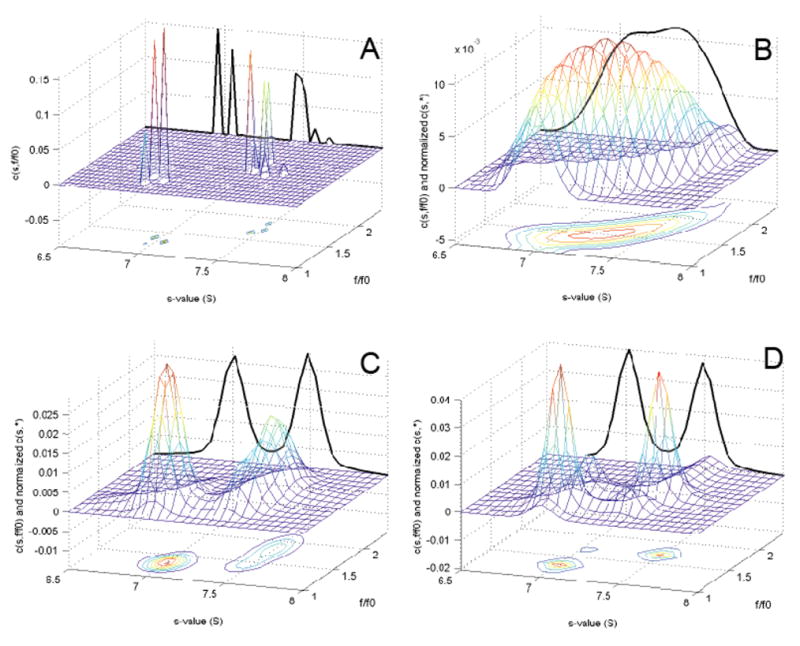
Two-dimensional size-and-shape distribution with prior expectation. Sedimentation profiles were simulated for two species at equal loading concentration with dissimilar frictional ratio: 130 kDa, 7 S, f/f₀ = 1.32 and 220 kDa, 7.5 S, f/f₀ = 1.74, respectively, sedimenting in a 10 mm column at 45,000 rpm. Normally distributed noise at 0.005-fold the total loading concentration 1 was added. (A) Sedimentation data analyzed with a size-and-shape distribution c(s,f/f₀) (Eq. 4) without the use of regularization. Shown are the c(s,f/f₀) distribution, together with a contour line representation projected on the s-f/f₀-plane. The bold solid line in the far s-c-plane is the normalized general c(s,*) distribution, which is obtained from integration of c(s,f/f₀) along the f/f₀ axis (Eq. 5). (B) c(s,f/f₀) distribution with Tikhonov-Philips regularization at a confidence level of P = 0.7, but without the use of prior knowledge. (C) Size-and-shape distribution c^(P)(s,f/f₀) using prior knowledge about the s-values of the two species, implemented as Gaussian peaks in the prior expectation at 7.0 and 7.5 S, respectively, with widths of 0.2 S and amplitudes 10-fold above the uniform baseline prior. Tikhonov-Philips regularization was used at a confidence level of P = 0.7. (D) Size-and-shape distribution c^(P)(s,f/f₀) using prior knowledge about the s-values as in panel (C), and in addition prior knowledge about the existence of two f/f₀ values with Gaussian peaks at f/f₀ = 1.3 and 1.7, respectively. No knowledge was implemented about which s-value correlates with which f/f₀ value.

The potential of SV to detect trace amounts of oligomeric species with high sensitivity has important applications in the study of intermediates in the cooperative assembly of multi-protein complexes or aggregates of misfolded protein, for example, in the study of protein fibrils and other structures, and in characterizing protein formulations in biotechnology. However, at very low concentrations, noise in the experimental data can obscure the precise sedimentation coefficients of trace components, complicating their quantitation and characterization ⁵². To study the use of prior expectations in this class of applications, we simulated the sedimentation profiles of 0.25% of a dimeric species sedimenting in the leading edge of the diffusionally broadened sedimentation boundary of a monomer (inset Figure 5 – note the axis break at 0.01/S). Without prior knowledge constraints, the c(s) distribution did not well resolve the dimer and showed broad features (Figure 5, solid black line), which resulted in relatively large relative errors of the concentration estimates from the peak areas (0.06% within the range from 10 S – 15 S versus the underlying 0.25%). In contrast, when we implemented the ME prior expectation from the known s-value of both the monomer and the dimer, the c^(P)(s) peak was well-developed and provided much better estimates for the dimer concentration (Figure 5, solid red line) (0.23% versus the underlying 0.25%). However, the concentration estimate for the dimer was found to depend on the amplitude of the Gaussian describing the prior expectation for the dimer. Also, the improvement was found to be only minor if no prior expectation was used to describe the knowledge of the mono-dispersity of the monomer (data not shown). Similar behavior was observed whether or not the monomer and dimer have the same frictional ratio. For the problem of trace oligomer detection, we found ME regularization to be superior to TP regularization.

Figure 5.

Detection of trace quantities of oligomers. Sedimentation profiles were generated for two species, a major monomeric species sedimenting at 7.0 S and a trace amount (0.25%) of a second dimeric species sedimenting at 10.0 S (in a 10 mm solution column, at 50,000 rpm, with f/f₀ ~ 1.3 for both species, and with a total loading signal of 1.0 with normally distributed noise of 0.005). The analysis was performed after optimization of f/f₀, allowing for systematic radial and time-dependent baseline offsets, and with ME regularization at a confidence level of P = 0.7. Shown are the common c(s) with uniform prior (blue solid line), and c^(P)(s) (red solid line) using the prior expectation from the known s-value of the monomer and dimer, implemented as Gaussians of width 0.1 and 0.5 S, respectively, and amplitudes of 100-fold the flat prior for the remaining distribution. The inset shows the complete distribution including the monomer peak (note the vertical axis break at 0.01), whereas the main panel is focused on the range of sedimentation coefficients for the oligomers. As a measure of the diffusional broadened boundary shape, inset also shows the least-squares ls-g*(s) (green solid line).

So far, we have considered stable macromolecular species. An increasingly important topic of hydrodynamic transport experiments by SV is protein interactions. Protein complexes can be distinguished with regard to their stability relative to the time-scale of sedimentation. Complexes behave as virtually stably sedimenting species in SV either if they exhibit dissociation rate constants slower than ~1/hour ⁶⁸, or if concentrations are far above K_D such that dissociating complexes will be driven by mass-action law to be readily re-assembled and their time-averaged state to be close to that of the complex. We have previously used as a model problem the SV data from the interaction of two peptides derived from the proline-rich domain of the adaptor protein SLP-76 and the SH3 domain of PLCγ, and shown by multi-signal analysis ³⁴ and by direct global Lamm equation modeling ⁶⁸ that it forms 1:1 complexes that are long-lived on the time-scale of sedimentation. In the present context we focus on the interference optical data only (Figure 6A) as a model to assess the potential impact of prior knowledge on their analysis.

Figure 6.

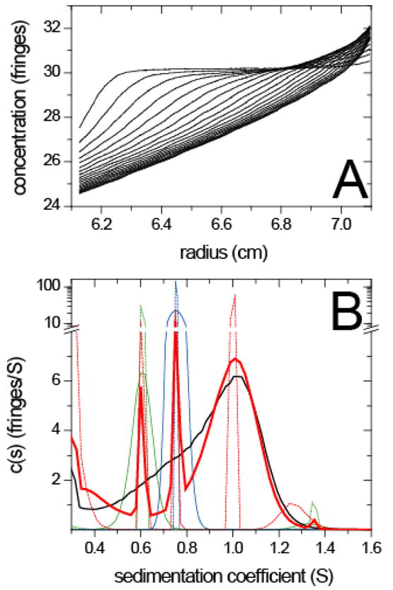
Prior knowledge in the analysis of interacting macromolecules forming dynamically stabilized complexes. (A) Interference optical sedimentation velocity data of a mixture of peptides derived from the adaptor protein SLP-76 (11.7 kDa) and PLC-γ (7.4 kDa) which form complexes with 1:1 stoichiometry ³⁴,⁶⁸. For experimental details, see 34. (B) The conventional sedimentation coefficient distribution c(s) are shown for the mixture (black solid line) and from separate experiments with SLP-76 (green solid line) and PLC-γ (blue solid line). In a secondary analysis, the c^(Pδ)(s) distributions of the separate experiments based on the prior expectation that each protein sample is monodisperse are shown as green and blue dotted lines, respectively. The prior expectation that both free protein species are mono-disperse and should exhibit the same sharp peaks in the mixture as in the individual experiments is then implemented in the c^(P)(s) distribution calculated from the sedimentation data of the mixture (solid red line). A tertiary analysis was applied to the mixture by calculating the c^(Pδ)(s) with the prior expectation that all peaks in the secondary analysis (solid red line) should be sharp peaks from mono-disperse species (dotted red line).

Figure 6B shows the c(s) distributions of the individual proteins (solid blue and green lines) studied in separate experiments (original fringe data not shown). From an initial c(s) analysis, the s_w of the peaks could be extracted and for mono-disperse samples the prior expectation can be implemented that the peaks should be a discrete representation of δ-funcions as described in Eq. 12. The result of this secondary analysis for the individual protein samples, c^(Pδ), is shown as dotted blue and green lines, respectively. This model provided a good description of the data, but indicated a trace impurity at 1.35 S in the SLP-76 sample. For the mixture, the standard c(s) distribution with uniform prior shows only a single broad peak (solid black line), indicative of complex formation but not suitable for further characterization beyond the overall s_w. Implementing the s-values of the free species as prior expectation, we obtained the c^(P)(s) distribution shown as red solid line. With the prior knowledge on the free species, the complex peak emerges more clearly. The data analysis can proceed further by using the additional prior expectation that the complex forms a single species, as well (red dotted line). This causes an additional small peak at 1.25 S to emerge, which could be either a result of real aggregation, or represent an ‘edge’ effect from the incorrect single-species constraint applied to ensembles with micro-heterogeneity (here likely conformational heterogeneity of the highly elongated peptides). Thus, the gradual implementation of prior expectations from certain knowledge (s-values of the free species) or hypothesized (mono-dispersity of the s-values of the complex) allows one to draw more detailed conclusions from this single data set.

Sedimenting systems of interacting macromolecules with fast chemical kinetics on the time-scale of sedimentation (k_off > 10⁻³/sec ⁶⁸) show sedimentation patterns much different from those of stable or dynamically stabilized species. For a two-component mixture, only two boundary components are expected (independent of the number of complex species): (1) the ‘undisturbed boundary’ consisting of the sedimentation of one free species (but not necessarily the species in molar excess); and (2) the ‘reaction boundary’ consisting of a mixture of free species and complex(es) that (in the ‘constant-bath’ approximation) sediments and diffuses approximately like a single species ⁶⁹ reflecting the time-average state of the sedimenting macromolecules. In a diffusion-free approximation, Gilbert & Jenkins have shown how to predict the ‘asymptotic boundaries’, i.e. approximations for the detailed sedimentation coefficient distributions of all species in the reaction boundary ⁶². More recently, we have shown that the c(s) distribution can be understood as an approximation of these asymptotic boundaries, and that isotherms derived from the weight-average s-values and the amplitudes of the asymptotic boundaries calculated in Gilbert-Jenkins theory can be fitted to the corresponding quantities derived from c(s) analysis of experimental data ⁶¹. In the present context, we asked the question whether the asymptotic boundary profiles from Gilbert-Jenkins theory based on an initial c(s) analysis can be used as prior expectation in a refined analysis of data by c^(P)(s). In this context, open problems arising from the need for regularization in c(s) are (1) to what extent c(s) and the asymptotic boundary correspond to each other in the detailed shape (i.e. whether regularization would obscure possible inconsistencies); and (2) the lack of resolution of the undisturbed and the reaction boundary at low signal-to-noise ratios. These questions can be addressed with the tool of inserting prior probabilities in c(s).

We simulated sedimentation profiles for a rapidly interacting system of two macromolecules forming a complex with 1:1 stoichiometry, using finite element solutions to systems of Lamm equations incorporating appropriate chemical reaction terms ⁶⁸ and added normally distributed noise. The parameters were chosen as those in Figure 6 of ⁶¹ (except for using an instantaneous reaction rate): small interacting proteins with moderately high affinity such that at concentrations lower than K_D only a poor signal-to-noise ratio was achieved. In the conventional c(s), despite the deconvolution of diffusion, at low concentrations the ME regularization favors broader peaks consistent with the signal-to-noise ratio and the bimodal boundary structure cannot be recognized (see Figure 6 of ⁶¹, and inset in Figure 7). In contrast, when using the Gilbert-Jenkins theory based prior expectation, the c^(P)(s) exhibits sharp peaks for the undisturbed and the reaction boundaries. In practice, the amplitudes of these peaks could be used as additional data points in a refined isotherm analysis. It is noteworthy that at concentrations ≤ K_D, the c^(P)(s) peak shapes are quite consistent with the asymptotic boundaries from Gilbert-Jenkins theory. At concentrations > K_D, additional small peaks can be discerned in c^(P)(s) which highlight deviations from the results of Gilbert-Jenkins theory and from c(s) approach. However, as shown previously, the weight-average s-values over the reaction boundary virtually coincide in Gilbert-Jenkins theory and c(s) ⁶¹, which is consistent with the observation of c^(P)(s) showing extra peaks on both sides of the asymptotic boundary. For this problem, similar results were obtained for ME and TP regularization.

Figure 7.

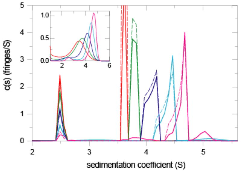
Prior knowledge in the analysis of interacting macromolecules reacting rapidly on the time-scale of sedimentation. Sedimentation data were simulated using Lamm equations incorporating reaction terms for the sedimentation of a 2.5 S, 25 kDa protein interacting with a 3.5 S, 40 kDa protein to form a 5 S complex with 1:1 stoichiometry at a K _D of 3 μM. Sedimentation was simulated to take place in a 10 mm column at 50,000 rpm, as would be detected with the interference optical system from 12 mm centerpieces at a noise of 0.01 fringes. Sedimentation profiles (not shown) were calculated for equimolar protein concentrations of 0.3 μM (red), 1 μM (green), 3 μM (dark blue), 10 μM (cyan), and 30 μM (magenta), leading to total signals of approximately 0.07, 0.22, 0.65, 2.2, and 6.5 fringes, respectively. In the inset is shown the conventional c(s) analysis with ME regularization with P = 0.9. All distributions are scaled relative to the loading concentration. The main panel shows the c^(P)(s) distributions (bold solid lines) using the asymptotic boundary profiles calculated by Gilbert-Jenkins theory (dashed thin lines) as prior knowledge.

Finally, we examined the case that for a rapidly interacting system the time-scale of the reaction is not recognized, and false prior expectations are used in the analysis that assume the presence of stable or dynamically stabilized species. This is illustrated in Figure 8 for a rapid monomer-dimer self-association, where we used the same synthetic data generated previously as a model to demonstrate the behavior of the conventional c(s): it exhibits peaks at a position intermediate to that of the monomer and dimer, with increasing s-values at higher concentrations ⁷⁰. With the false prior expectation that the monomer and dimer s-values should be populated (dotted lines in Figure 8), c^(P*⁾(s) distributions as shown as solid lines in Figure 8 were observed. Similar to the conventional c(s), the dominating peaks are at the intermediate s-values, in a concentration-dependent location. As outlined previously, this behavior would indicate the presence of a rapid interaction on the time-scale of sedimentation, contrasting with the impostor prior. Only in the range of s-values very close to that of the monomer and dimer did the prior expectation effect a condensing of the distribution to form a peak close (but not precisely at) the position of the monomer and dimer s-values. This result demonstrates that for fast reactions the observation of s-values intermediate to that of the interacting species (close to the time-average state, with a distribution predicted from Gilbert-Jenkins theory) is highly significant information contained in the experimental data. This feature of the experimental data is not subject to the room for interpretation that arises from posing the analysis as the Fredholm integral equation, and cannot be eliminated by incorrectly assigned prior expectations.

Figure 8.

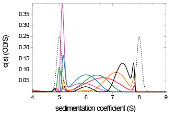
Analysis of a rapidly interacting monomer/dimer system with impostor prior expectation. Sedimentation velocity data were simulated with Lamm equation solutions incorporating reaction terms for a 100 kDa monomer in instantaneous equilibrium with a dimer, with an equilibrium constant of 2 μM, sedimenting at 50,000 rpm. Simulation parameters were chosen to mimic absorption optical detection at different wavelengths, with 0.01 OD noise (see ⁷⁰). Concentrations were 0.2 μM (magenta), 0.5 μM (blue), 1 μM (green), 2 μM (red), 5 μM (orange), and 10 μM (black). Unless proteins are very elongated, at the highest concentration of 1 mg/ml simulated here repulsive hydrodynamic non-ideality can still be neglected. Shown are the sedimentation coefficient distributions c^(P*⁾(s) (solid lines) using the impostor prior expectation that sedimentation proceeds as if there was stable monomeric and dimeric species (dotted line). Regularization was using the TP method on a confidence level of P = 0.7.

DISCUSSION

As shown in the present study, the choice of prior knowledge can have a profound influence on the sedimentation coefficient and size-and-shape distributions derived from experimental sedimentation velocity analytical ultracentrifugation data, as well as molecular weight distributions derived from sedimentation equilibrium data. Because of this, we suggest different symbols (c^(P)(M), c^(P)(s), c^(Pδ)(s), c^(P)(s,f_r), etc.) for distributions that deviate from the conventional assumption of uniform prior and propose it should be applied with transparent origin of the prior knowledge implemented, and with clarity about the flow of information.

Since the regularization with explicit prior expectations is new in AUC analysis, we recapitulate the concept and assumptions. As is well-known in the numerous disciplines of biophysics, geophysics, astronomy, image processing and tomography where models for the observed data consist of Fredholm integral equations with more or less smooth kernels, frequently many different solutions (i.e. parameter distributions) exist that can explain the observed data almost equally well and are indistinguishable within the statistical limits imposed by the noise of the data acquisition. Commonly, strictly the best-fit solution is not realistic or at least not reliable as it tends to be dominated by series of large spikes, the position and gross features of which may be determined by the details of the noise as well as the numerical discretization of the integral equation. Such behavior is to be expected from mathematical considerations (Lemma of Riemann-Lebesgue ^39,44), and shows up in familiar form in SV analysis. Regularization is the introduction of a bias to select, among all possible statistically indistinguishable solutions, the one that conforms best with a pre-defined property. In the form that was previously introduced in SV analysis, the bias defaulted towards the distribution with minimal information content or maximal smoothness, such that adventitious spikes in the solutions and noise amplification would be maximally suppressed. This is achieved by assigning each parameter value an equal prior expectation, and minimizing the deviation from this flat prior expectation. (From a pragmatic point of view, TP and ME differ in the mathematical expression that penalizes this deviation, and in their implicit prior expectations ⁴⁶.) Guided by Occam’s razor, this choice has proven to be remarkably powerful in the large literature of its application in SV analysis ³⁰, consistent with long-standing experience in many other disciplines. However, with consideration of specific knowledge available prior to and independently of the acquired data to be analyzed, the selection of the best solution from all possible ones can be made differently, by directing the bias towards the solution that is most consistent with the prior knowledge. According to Bayesian data analysis principles, this should result in the best estimate for the solution ⁴⁷.

It must be recognized, though, that the optimality of this estimate depends on the truth of the prior knowledge implemented. For example, the expectation that a pure protein sample should result in a mono-disperse sedimentation coefficient peak may be reasonable, but could be wrong in the presence of microheterogeneity regarding the mass (e.g., glycosylation or other modifications) or microheterogeneity regarding hydrodynamic properties arising from the existence of an ensemble of different conformations with slow interconversion. Such complicating factors may not be recognized by the experimenter, and it is difficult to assign strict probability values to their presence. Therefore, we have no recipe for the numerical value of the scaling factors for A_k (Eq. 11). However, when using ad hoc amplitude values varying between 10¹ and 10³-fold the baseline value, for SV analyses we found the balance between overall parsimony and honoring the prior expectation reasonable, and the results not to be overly sensitive to this parameter. For the same reason that there may be a small chance the prior expectation is not precisely true, we have examined in the present paper some cases how impostor prior can be recognized given sufficiently informative experimental data. Generally, the c^(P*⁾(s) distributions will deviate from the expected shape, for example, generating secondary peaks in c^(Pδ*⁾(s). Such information can be useful when testing the implications of a particular hypothesis (e.g. the mono-dispersity of a sample) on the data analysis. This provides significantly greater detail of information and flexibility as compared to the rigid implementation of fixed constraints (which can only be tested whether or not they are fully consistent with the experimental data by comparison of the final goodness-of-fit, but do not provide additional details in which way the constraint may be insufficient).

The source of the prior knowledge may be direct knowledge of species with certain s-values likely occurring in the solution, for example, from other samples studied side-by-side in the same rotor, or from analyses of other data from the same experiment, such as data acquired at a wavelength that selectively detects certain species, or back-of-the-envelope estimations of likely sedimentation coefficients of complexes based on hydrodynamic scaling law, such as the s ~ M^2/3 rule of thumb, or the expectation of a certain shape of the distribution (like the theoretical asymptotic boundaries). In some cases, however, the prior knowledge may be more indirect and not include the specific s-value, for example, the expectation of the mono-dispersity of the sample. Steinbach and colleagues have approached a similar problem by initially using a model with uniform prior, followed by adaptation of the observed peaks into the prior as Gaussians with reduced widths ⁷¹. This was implemented in the program MemExp for the analysis of life-time distributions ⁷². We have implemented this strategy in SEDFIT by automatic introduction of c(s) peaks as (discrete representations on a fixed grid) of delta-functions comprising the prior for c^(Pδ)(s), over the background of a flat baseline prior probability for parameters outside the specific range. The initial flat prior is maximally non-committal, but when studying distributions of intrinsically discrete parameters (such as molecular weights of biomacromolecules), by convention, the resulting broad features of the distribution are usually interpreted to reflect a discrete species observed at limited resolution, rather than a truly broad dispersion of parameter values.Footnote 3 Making this interpretation explicit, for example, by calculating c^(Pδ)(s), allows us to test this conventional interpretative step, and to examine more quantitatively whether or not a discrete species model could really explain all aspects of the data, while continuing to make minimal assumptions for the s-values outside the peak.

SV data have information in different dimensions – sedimentation, diffusion and extinction coefficients. From the systems studied in the present paper, we believe that they are largely independent with regard to the tools to incorporate prior knowledge and problems arising from incorrect assumptions. While the present study was concerned mainly with the introduction of prior knowledge on the sedimentation coefficients, additional prior knowledge can be implemented for the description of diffusion, either via hydrodynamic scaling laws, by using c(s) models with multi-modal frictional ratios (available in different variations in SEDFIT and SEDPHAT), or by directly introducing prior knowledge on the frictional ratio distribution for calculating size-and-shape distribution (Figure 4D). It should be noted that the approach with the least amount of implicit prior knowledge is the general c(s,*), which does not make any assumptions about diffusion coefficients and extracts from the experimental data alone the information for the deconvolution of diffusion in the sedimentation coefficient distributions. We have not yet implemented the application of the prior probabilities to the multi-signal c_k(s) analysis ³⁴, but the same principles should apply and we would expect similar advantage as in the c(s) and c(s,f/f₀) methods. However, at a simpler level it is possible at the current state to use, for example, a c(s) distribution determined from a signal with superior signal-to-noise ratio (leading to higher resolution) as a prior in the analysis of a second signal with lower signal-to-noise ratio (with conventional regularization exhibiting lower resolution) from the same sedimentation experiment, in order to discern in detail the differences and presence of additional species.

It is of interest to compare different regularization approaches in light of AUC analysis and the possibility of incorporating prior knowledge. Among ME and TP regularization, previously, it seemed preferable to choose ME for mixtures of discrete proteins, due to the non-linear nature of the entropy penalty term allowing the description of sharper isolated peaks ^21,46. Conversely, TP seemed advantageous for intrinsically broader distributions such as polydisperse polymers or diffusionally-broadened apparent sedimentation coefficient distributions ls-g*(s) due to the well-known tendency of ME with uniform prior to generate ripples in broad distributions ^{46,71,73–75} (see below). Since the prior expectation of sharp peaks can be explicitly implemented in both ME and TP c^(Pδ)(s) equally well as a second stage analysis from an initial conventional c(s), from a pragmatic point of view the differences between TP and ME seem to become smaller and TP more attractive for its usually shorter computational time (even though there are fundamental differences in the concept of the two methods ⁴⁶), provided that prior knowledge on the discrete nature of the sedimenting species is warranted.Footnote 4 However, we found that for trace detection of small peaks in the presence of unrelated large peaks, ME regularization performed better (see below).

Historically, data transformations have been devised for estimating sedimentation coefficient distributions from experimental SV data ^76,77 (at different levels of approximation for diffusion resulting in overall lower resolution; for a comparison see 28), and recently a new data transformation approach for the decomposition of exponentials was reported ⁷⁸, potentially applicable to SE. However, the direct numerical inversion of the integral equation in combination with regularization has distinct advantages, which, besides preserving the statistical weights of the data ⁷⁹, include the possibility for extension to global fits of multiple data sets ⁸⁰ and multi-dimensional distributions ^27,81,82, and the well-known possibility to introduce prior knowledge and prior expectations as focused on in the present work. Both factors can significantly improve the robustness of the method, as well as the resolution and level of reliable detail extracted from the data.

Another, non-traditional approach for solving the Fredholm integral equation Eq. 4 was recently described for application to SV analysis. Demeler and colleagues have embarked on a heuristic strategy to divide the parameter space in a series of subsets, perform a least-squares analysis for each subset, and merge the positive parameters into a final analysis ^83–85. This was motivated by the possibility of parallel computing in this scheme, and by the saving in computational effort arising from the exclusion of sections of the parameter space in the final analysis. However, considering that different parameter regions in Eqs. 1 and 4 can be notoriously cross-correlated, it is an open question whether the final solution will in fact be the best-fit solution – or even of statistically indistinguishable quality to the best-fit solution considering the full parameter space – as would be required for a reliable data interpretation. Further, as Demeler’s strategy permits to refine the discretization in certain parameter regions surrounding the main peaks, if used in the absence of regularization, this method would be expected to exacerbate the amplification of noise in the data into large, artifactual spikes dominating the final solution (see above). Footnote 5

In the present work we have further explored two particular applications of prior probabilities in ultracentrifugal size-distribution analysis. The detection of trace oligomeric species in protein preparations has attracted significant attention, due to the importance of misfolded oligomers forming nuclei for protein fibrillation or aggregation. AUC experiments in conjunction with the c(s) analysis have found wide-spread use as a method orthogonal to traditional size-exclusion chromatography, providing only low throughput but offering the advantage of the absence of surfaces and matrices ^31–33. In the present study, using simulated data with a very low level of trace dimer close to the detection limit, we found that improved detection limits can be achieved when departing from the conventional ME regularization with uniform prior. Although regularization is essential for a reliable data analysis, it appears that the peak broadening of the main peak afforded by the noise level (even though less in ME than in TP regularization) can cause a de-localized pattern of peaks for the trace contaminants at higher s-values. This effect can be effectively eliminated when using prior knowledge of the s-value of the main peak to permit its description as a very sharp peak (delta-function), in conjunction with the localization of the dimer peak by introducing prior knowledge on its s-value. The concept of introduction of prior knowledge for enhanced sensitivity of trace detection will be explored in more detail elsewhere (P. Brown, manuscript in preparation).

This effect appears closely related to the observation of discrete peaks causing ripples in well-separated neighboring broad distributions, as reported, for example, in the context of time-resolved fluorescence ⁷¹, autocorrelation functions in dynamic light scattering ^74,75, and astronomical image restoration ⁴⁶. Interestingly, in these fields it was found that the introduction of prior knowledge that permits sharpening of the discrete peaks will diminish the ripples in the broad distribution ^46,71,75 (see, e.g. Figure 2 of ⁷¹). A more difficult problem is that of a main, sharp peak overlapping a broad distribution, and different computational strategies have been reported, including separate regularization of the peak and the broad background or by modifications to the entropy constraint to modulate the nonlinearity in the signal-dependence of the regularization ^46,86. By analogy, such advanced strategies may be useful for future SV analysis with improved resolution and sensitivity to trace species sedimenting at s-values similar to the main peak.

For trace detection, it may be of interest not only to use prior knowledge about the s-values of monomers and oligomers, but also to match the area under the monomer and oligomer peaks to the relative concentrations measured by other techniques, for example, by chromatography. Although we have not pursued this approach in the present work, it may allow to directly test whether chromatographic and ultracentrifugal trace detection is consistent for a given sample: any departure from the prior would indicate significant differences between the two.

Finally, we used the c(s) with prior expectation to address a theoretical question regarding the correspondence between the c(s) analysis and the asymptotic boundaries from Gilbert-Jenkins theory for rapidly reacting systems. Based on the ‘constant-bath’ approximation of the Lamm equation for reacting systems, we have argued previously that diffusional deconvolution in c(s) is successful despite the reaction fluxes between different species not being accounted for in the kernel of Eq. 1, and that the sedimentation coefficient distributions c(s) so derived from experimental data should be closely related to the predictions from Gilbert and Jenkins in a diffusion-free approximation for the sedimentation of the reacting system. However, the finite signal-to-noise ratio of the experimental data causes the conventional regularization to generate broadened c(s) peaks, which cannot be directly compared with the asymptotic boundaries from Gilbert-Jenkins theory. The tool of prior expectation allows us to overcome this limitation in c^(P)(s) and to directly display features of c(s) that are inconsistent with Gilbert-Jenkins theory. While at concentrations smaller than or approximately at K_D the asymptotic boundaries provide an excellent description, at concentrations higher than K_D they cannot be described exactly by Gilbert-Jenkins asymptotic boundaries. Extra peaks outside the sedimentation coefficient range predicted by Gilbert-Jenkins theory appear in c^(P)(s), which seem to point to unaccounted diffusional transport of the reacting system at finite times, which neither Gilbert-Jenkins theory nor c(s) will describe precisely. However, we have shown previously that there exists an excellent quantitative correspondence of both the weight-average sedimentation coefficient averaged over the complete reaction boundary, as well as the amplitude of the reaction boundary, between the c(s) distributions and the predictions from Gilbert-Jenkins theory ⁶¹. We believe that these two quantities are left invariant because of the bi-directional nature of the diffusion processes.

The correspondence of the amplitude and weight-average s-values of the reaction boundary is the basis for the quantitative analysis of diffusion-deconvoluted reaction boundaries in c(s) with isotherms derived from Gilbert-Jenkins theory, which exploits the bimodal boundary shape and thereby significantly extends (and can be combined in a global analysis with) the mass balance analysis of the overall weight-average s-value, without requiring a detailed interpretation of the boundary shape (or c(s) shape, respectively) ⁶¹. The present strategy strengthens this approach by helping to resolve the undisturbed and the reaction boundary even at very low concentrations, where previously the regularization with flat prior failed to resolve the two peaks ⁶¹.

In summary, we have implemented and examined the use of prior expectation in the regularization for ultracentrifugal size distributions. Prior information may be available from a variety of sources, including theoretical considerations, experimental data, or special properties of the macromolecules under study. Our results indicate that this can substantially increase the resolution and sensitivity of the analysis. In contrast to the implementation of fixed constraints, such as a discrete species model, the prior expectation introduces only a subtle bias, not leading to a statistically significant reduction of the quality of fit, and permitting the experimental data to supplement the prior expectation with additional essential features or essentially contradict it altogether. Even in the absence of certain prior knowledge, this more flexible strategy allows to examine the consequences of different alternative hypotheses. We believe that this approach provides a flexible tool that should prove highly useful for the study of biological macromolecules by analytical ultracentrifugation.

References

- 1.Lebowitz J, Lewis MS, Schuck P. Protein Sci. 2002;11:2067–2079. doi: 10.1110/ps.0207702. [DOI] [PMC free article] [PubMed] [Google Scholar]
- 2.Howlett GJ, Minton AP, Rivas G. Curr Opin Chem Biol. 2006;10:430–436. doi: 10.1016/j.cbpa.2006.08.017. [DOI] [PubMed] [Google Scholar]
- 3.Perez Sanchez H, Tatarenko K, Nigen M, Pavlov G, Imberty A, Lortat-Jacob H, Garcia de la Torre J, Ebel C. Biochemistry. 2006;45:13227–13238. doi: 10.1021/bi061490w. [DOI] [PubMed] [Google Scholar]
- 4.Pavlov GM, Korneeva EV, Yevlampieva NP. Int J Biol Macromol. 1994;16:318–323. doi: 10.1016/0141-8130(94)90063-9. [DOI] [PubMed] [Google Scholar]
- 5.Harding SE. Carbohydr Res. 2005;340:811–826. doi: 10.1016/j.carres.2005.01.027. [DOI] [PubMed] [Google Scholar]
- 6.Patel TR, Picout DR, Ross-Murphy SB, Harding SE. Biomacromolecules. 2006;7:3513–3520. doi: 10.1021/bm060674n. [DOI] [PubMed] [Google Scholar]
- 7.Clay O, Douady CJ, Carels N, Hughes S, Bucciarelli G, Bernardi G. Eur Biophys J. 2003;32:418–426. doi: 10.1007/s00249-003-0294-y. [DOI] [PubMed] [Google Scholar]
- 8.Schultes EA, Spasic A, Mohanty U, Bartel DP. Nat Struct Mol Biol. 2005;12:1130–1136. doi: 10.1038/nsmb1014. [DOI] [PubMed] [Google Scholar]
- 9.Pavlov GM, Zaitseva II, Michailova NA, Rjumtsev EI. Polymer. 2004;45:1159–1166. [Google Scholar]
- 10.Schubert D, Tziatzios C, Schuck P, Schubert US. Chem Eur J. 1999;5:1377–1383. [Google Scholar]
- 11.Meier MAR, Hofmeier H, Abeln CH, Tziatzios C, Rasa M, Schubert D, Schubert US. E-Polymers. 2006 2006 May 16;(Art No 016) [Google Scholar]
- 12.Vogel V, Langer K, Balthasar S, Schuck P, Machtle W, Haase W, van den Broek JA, Tziatzios C, Schubert D. ProgColloid Polymer Sci. 2002;119:31–36. [Google Scholar]
- 13.Pavlov GM, Errington N, Harding SE, Korneeva EV, Roy R. Polymer Science Series A. 2001;43:118–123. [Google Scholar]
- 14.Kasemi E, Zhuang W, Rabe JP, Fischer K, Schmidt M, Colussi M, Keul H, Yi D, Colfen H, Schluter AD. J Am Chem Soc. 2006;128:5091–5099. doi: 10.1021/ja057964g. [DOI] [PubMed] [Google Scholar]
- 15.Berkowitz SA, Philo JS. Anal Biochem. 2006 doi: 10.1016/j.ab.2006.11.031. [DOI] [PubMed] [Google Scholar]
- 16.Schachman HK. Nature. 1989;341:259–260. [Google Scholar]
- 17.Behlke J, Ristau O. Biophys J. 1997;72:428–434. doi: 10.1016/S0006-3495(97)78683-1. [DOI] [PMC free article] [PubMed] [Google Scholar]
- 18.Philo JS. Biophys J. 1997;72:435–444. doi: 10.1016/S0006-3495(97)78684-3. [DOI] [PMC free article] [PubMed] [Google Scholar]
- 19.Schuck P. Biophys J. 1998;75:1503–1512. doi: 10.1016/S0006-3495(98)74069-X. [DOI] [PMC free article] [PubMed] [Google Scholar]
- 20.Schuck P, Demeler B. Biophys J. 1999;76:2288–2296. doi: 10.1016/S0006-3495(99)77384-4. [DOI] [PMC free article] [PubMed] [Google Scholar]
- 21.Schuck P. Biophys J. 2000;78:1606–1619. doi: 10.1016/S0006-3495(00)76713-0. [DOI] [PMC free article] [PubMed] [Google Scholar]
- 22.Demeler B, Behlke J, Ristau O. Methods in Enzymology. 2000;321:36–66. doi: 10.1016/s0076-6879(00)21186-5. [DOI] [PubMed] [Google Scholar]
- 23.Schuck P. Euroconference. Advances in Analytical Ultracentrifugation and Hydrodynamics; Autrans, France: 2002. [Google Scholar]
- 24.Behlke J, Ristau O. Biophys Chem. 2002;95:59–68. doi: 10.1016/s0301-4622(01)00248-4. [DOI] [PubMed] [Google Scholar]
- 25.Stafford WF, Sherwood PJ. Biophys Chem. 2004;108:231–243. doi: 10.1016/j.bpc.2003.10.028. [DOI] [PubMed] [Google Scholar]
- 26.Cao W, Demeler B. Biophys J. 2005;89:1589–1602. doi: 10.1529/biophysj.105.061135. [DOI] [PMC free article] [PubMed] [Google Scholar]
- 27.Brown PH, Schuck P. Biophys J. 2006;90:4651–4661. doi: 10.1529/biophysj.106.081372. [DOI] [PMC free article] [PubMed] [Google Scholar]
- 28.Schuck P, Perugini MA, Gonzales NR, Howlett GJ, Schubert D. Biophys J. 2002;82:1096–1111. doi: 10.1016/S0006-3495(02)75469-6. [DOI] [PMC free article] [PubMed] [Google Scholar]
- 29.Schuck P. In: Modern Analytical Ultracentrifugation: Techniques and Methods. Scott DJ, Harding SE, Rowe AJ, editors. The Royal Society of Chemistry; Cambridge: 2006. pp. 26–50. [Google Scholar]
- 30.Schuck P. 2007 http://www.analyticalultracentrifugation.com/references.htm.
- 31.Berkowitz SA. Aaps J. 2006;8:E590–605. doi: 10.1208/aapsj080368. [DOI] [PMC free article] [PubMed] [Google Scholar]
- 32.Gabrielson JP, Brader ML, Pekar AH, Mathis KB, Winter G, Carpenter JF, Randolph TW. J Pharm Sci. 2006;96:268–279. doi: 10.1002/jps.20760. [DOI] [PubMed] [Google Scholar]
- 33.Liu J, Andya JD, Shire SJ. Aaps J. 2006;8:E580–589. doi: 10.1208/aapsj080367. [DOI] [PMC free article] [PubMed] [Google Scholar]
- 34.Balbo A, Minor KH, Velikovsky CA, Mariuzza R, Peterson CB, Schuck P. Proc Natl Acad Sci U S A. 2005;102:81–86. doi: 10.1073/pnas.0408399102. [DOI] [PMC free article] [PubMed] [Google Scholar]
- 35.Minor KH, Schar CR, Blouse GE, Shore JD, Lawrence DA, Schuck P, Peterson CB. J Biol Chem. 2005;31:28711–28720. doi: 10.1074/jbc.M500478200. [DOI] [PMC free article] [PubMed] [Google Scholar]
- 36.Houtman JC, Yamaguchi H, Barda-Saad M, Braiman A, Bowden B, Appella E, Schuck P, Samelson LE. Nat Struct Mol Biol. 2006;13:798–805. doi: 10.1038/nsmb1133. [DOI] [PubMed] [Google Scholar]
- 37.deka RK, Brautigam CA, Tomson FL, Lumpkins SB, Tomchick DR, Machius M, Norgard MV. J Biol Chem. 2007;Epub:M610215200. doi: 10.1074/jbc.M610215200. [DOI] [PubMed] [Google Scholar]
- 38.Hansen PC. Inverse Probl. 1992;8:849–872. [Google Scholar]
- 39.Provencher SW. Comp Phys Comm. 1982;27:213–227. [Google Scholar]
- 40.Provencher SW. Makromol Chem. 1979;180:201–209. [Google Scholar]
- 41.Provencher SW. Comp Phys Comm. 1982;27:229–242. [Google Scholar]
- 42.Jaynes ET. Phys Rev. 1957;106:620–630. [Google Scholar]
- 43.Mohommad-Djafari . Bayesian inference and maximum entropy methods in science and engineering. American Institute of Physics; New York: 2001. [Google Scholar]
- 44.Phillips DL. Assoc Comput Mach. 1962;9:84–97. [Google Scholar]
- 45.Hansen PC. Rank-deficient and discrete ill-posed problems: Numerical aspects of linear inversion. SIAM; Philadelphia: 1998. [Google Scholar]
- 46.Narayan R, Nityananda R. Ann Rev Astron Astrophys. 1986;24:127–170. [Google Scholar]
- 47.Sivia DS. Bayesian Tutorial. Oxford University Press; Oxford: 1996. Data Analysis. [Google Scholar]
- 48.Kaipio JP, Kolehmainen V, Vauhkonen M, Somersalo E. Inverse problems. 1999;15:713–729. [Google Scholar]
- 49.Li A, Miller EL, Kilmer ME, Brukilacchio TJ, Chaves T, Stott J, Zhang Q, Wu T, Chorlton M, Moore RH, Kopans DB, Boas DA. Applied Optics. 2003;42:5181–5190. doi: 10.1364/ao.42.005181. [DOI] [PubMed] [Google Scholar]
- 50.Doyley MM, Srinivasan S, Dimidenko E, Soni N, Ophir J. Phys Med Biol. 2006;51:95–112. doi: 10.1088/0031-9155/51/1/007. [DOI] [PubMed] [Google Scholar]
- 51.Jaynes ET. IEEE Transactions on Systems Science and Cybernetics. 1968;4:227–241. [Google Scholar]
- 52.Dam J, Schuck P. Methods Enzymol. 2004;384:185–212. doi: 10.1016/S0076-6879(04)84012-6. [DOI] [PubMed] [Google Scholar]
- 53.Boukari H, Nossal R, Sackett DL, Schuck P. Physical Review Letters. 2004;93:098106. doi: 10.1103/PhysRevLett.93.098106. [DOI] [PubMed] [Google Scholar]
- 54.Greive SJ, Lins AF, von Hippel PH. J Biol Chem. 2005;280:36397–36408. doi: 10.1074/jbc.M507146200. [DOI] [PubMed] [Google Scholar]
- 55.Chou CY, Jen WP, Hsieh YH, Shiao MS, Chang GG. J Biol Chem. 2006;281:13333–13344. doi: 10.1074/jbc.M511077200. [DOI] [PubMed] [Google Scholar]
- 56.Schuck P. 2007 www.analyticalultracentrifugation.com.
- 57.Balbo A, Schuck P. In: Protein-Protein Interactions. Golemis E, Adams PD, editors. Cold Spring Harbor Laboratory Press; Cold Spring Harbor, New York: 2005. pp. 253–277. [Google Scholar]
- 58.Lamm O. Ark Mat Astr Fys. 1929;21B(2):1–4. [Google Scholar]
- 59.Schuck P. Biophys Chem. 2004;108:187–200. doi: 10.1016/j.bpc.2003.10.016. [DOI] [PubMed] [Google Scholar]
- 60.Schuck P. Biophys Chem. 2004;187:201–214. doi: 10.1016/j.bpc.2003.10.017. [DOI] [PubMed] [Google Scholar]
- 61.Dam J, Schuck P. Biophys J. 2005;89:651–666. doi: 10.1529/biophysj.105.059584. [DOI] [PMC free article] [PubMed] [Google Scholar]
- 62.Gilbert GA, Jenkins RC. Nature. 1956;177:853–854. doi: 10.1038/177853a0. [DOI] [PubMed] [Google Scholar]
- 63.Svedberg T, Pedersen KO. The ultracentrifuge. Oxford University Press; London: 1940. [Google Scholar]
- 64.Vistica J, Dam J, Balbo A, Yikilmaz E, Mariuzza RA, Rouault TA, Schuck P. Anal Biochem. 2004;326:234–256. doi: 10.1016/j.ab.2003.12.014. [DOI] [PubMed] [Google Scholar]
- 65.Press WH, Teukolsky SA, Vetterling WT, Flannery BP. Numerical Recipes in C. 2. University Press; Cambridge: 1992. [Google Scholar]
- 66.Gilbert LM, Gilbert GA. Methods Enzymol. 1978;48:195–211. doi: 10.1016/s0076-6879(78)48011-5. [DOI] [PubMed] [Google Scholar]
- 67.Schuck P, Rossmanith P. Biopolymers. 2000;54:328–341. doi: 10.1002/1097-0282(20001015)54:5<328::AID-BIP40>3.0.CO;2-P. [DOI] [PubMed] [Google Scholar]
- 68.Dam J, Velikovsky CA, Mariuzza R, Urbanke C, Schuck P. Biophys J. 2005;89:619–634. doi: 10.1529/biophysj.105.059568. [DOI] [PMC free article] [PubMed] [Google Scholar]
- 69.Fujita H. Foundations of ultracentrifugal analysis. John Wiley & Sons; New York: 1975. [Google Scholar]
- 70.Schuck P. Anal Biochem. 2003;320:104–124. doi: 10.1016/s0003-2697(03)00289-6. [DOI] [PubMed] [Google Scholar]
- 71.Steinbach PJ, Ionescu R, Matthews CR. Biophys J. 2002;82:2244–2255. doi: 10.1016/S0006-3495(02)75570-7. [DOI] [PMC free article] [PubMed] [Google Scholar]
- 72.Steinbach PJ. 2007. [Google Scholar]
- 73.Amato U, Hughes W. Inverse Problems. 1991;7:793–808. [Google Scholar]
- 74.Johnsen RM, Brown W. In: Laser Light Scattering in Biochemistry. Harding SE, Sattelle DB, Bloomfield VA, editors. The Royal Society of Chemistry; Cambridge: 1992. pp. 77–91. [Google Scholar]
- 75.Provencher SW. In: Laser light scattering in biochemistry. Harding SE, Satelle DB, Bloomfield VA, editors. The Royal Society of Chemistry; Cambridge, U.K: 1992. pp. 92–111. [Google Scholar]
- 76.van Holde KE, Weischet WO. Biopolymers. 1978;17:1387–1403. [Google Scholar]
- 77.Stafford WF. Anal Biochem. 1992;203:295–301. doi: 10.1016/0003-2697(92)90316-y. [DOI] [PubMed] [Google Scholar]
- 78.Zhou Y, Zhuang X. Biophys J. 2006;91:4045–4053. doi: 10.1529/biophysj.106.090688. [DOI] [PMC free article] [PubMed] [Google Scholar]
- 79.Provencher SW, Vogel RH. Mathematical Biosciences. 1980;50:251–262. [Google Scholar]
- 80.Stepanek P, Provencher SW. Macromol Symp. 2000;162:191–203. [Google Scholar]
- 81.Steinbach PJ. Biophys J. 1996;70:1521–1528. doi: 10.1016/S0006-3495(96)79714-X. [DOI] [PMC free article] [PubMed] [Google Scholar]
- 82.Svitel J, Boukari H, Van Ryk D, Willson RC, Schuck P. Biophys J. 2007;Epub doi: 10.1529/biophysj.1106.094615. [DOI] [PMC free article] [PubMed] [Google Scholar]
- 83.Brookes E, Demeler B. 15th International Symposium on Analytical Ultracentrifugation. London: 2006. [Google Scholar]
- 84.Brookes E, Boppana RV, Demeler B. Proceedings of the 206 ACM/IEEE conference on supercomputing. Tampa; Florida: 2006. p. 81. [Google Scholar]
- 85.Demeler B. 2007 http://www.ultrascan.uthscsa.edu.
- 86.Steinbach PJ. Journal of Chemical Information and Computer Sciences. 2002;42:1476–1478. doi: 10.1021/ci025551i. [DOI] [PubMed] [Google Scholar]