

Summary
In this study, we characterize the adaptation of neurons in the cat lateral geniculate nucleus to changes in stimulus contrast and correlations. By comparing responses to high and low contrast natural scene movie and white noise stimuli, we show that an increase in contrast or correlations results in receptive fields with faster temporal dynamics and stronger antagonistic surrounds, as well as decreases in gain and selectivity. We also observe contrast- and correlation-induced changes in the reliability and sparseness of neural responses. We find that reliability is determined primarily by processing in the receptive field (the effective contrast of the stimulus), while sparseness is determined by the interactions between several functional properties. These results reveal a number of novel adaptive phenomena and suggest that adaptation to stimulus contrast and correlations may play an important role in visual coding in a dynamic natural environment.
Introduction
One of the biggest challenges facing the early visual pathway is the variability in the statistical properties of the natural environment. For example, the contrast in a particular area within the visual field is constantly changing due to local variations across the scene and global changes in overall viewing conditions. Similarly, while the stereotypical spatial and temporal correlations evident in the power spectra of natural visual scenes have been widely studied (power decreases with increasing frequency as 1/fα, with α typically between 1 and 3 (Field, 1987; Dong and Atick, 1995)), these correlations can vary dramatically depending on the specifics of the current environment. The variability of the natural environment requires that the early visual pathway employ an adaptive strategy, continuously changing its response properties to match the statistical properties of the current stimulus. Thus, in order to understand the function of the early visual pathway under natural viewing conditions, we must first understand its adaptive mechanisms.
Adaptive mechanisms are prominent in the early visual pathway. For example, a change in the contrast of the stimulus can evoke changes in the temporal dynamics and gain of neurons in the retina and thalamus (Shapley and Victor, 1979; Smirnakis et al., 1997; Solomon et al., 2004; Mante et al., 2005), and there is evidence that such changes are necessary to maintain the flow of visual information (Brenner et al., 2000; Fairhall et al., 2001). A recent study reported that changes in dynamics can also be evoked by specific stimulus patterns, indicating that visual neurons can also adapt to correlations in a manner that enhances sensitivity to novel stimuli (Hosoya et al., 2005). While some adaptive changes in the functional properties of the early visual pathway have been widely studied, there are a number of contrast- and correlation-induced effects that have not yet been characterized.
In this study, we examine the effects of adaptation to changes in stimulus contrast and correlations on the properties of neurons in the lateral geniculate nucleus (LGN) of the thalamus. To characterize adaptation in a functional context, we utilize the framework of a linear-nonlinear (LN) model. The LN model maps stimulus to firing rate through a cascade of a linear receptive field (RF) and a rectifying static nonlinearity (NL) with a gain and offset. While there are a number of similar models that provide a suitable functional description of visual encoding, we use this particular LN structure because its components can be related to functional properties such as spatial integration and temporal dynamics (RF) and selectivity (offset), or to underlying physiological properties such as conductance (gain) and baseline membrane potential (offset) (Brown and Masland, 2001; Baccus and Meister, 2002; Manookin and Demb, 2006; Beaudoin et al., 2007). Furthermore, this model has already been used successfully to characterize several of the functional and physiological changes associated with adaptation in the early visual pathway (Chander and Chichilnisky, 2001; Kim and Rieke, 2001; Zaghloul et al., 2005).
In this study, we fit LN models from responses to high and low contrast natural scene movie and white noise stimuli, and characterize the contrast- and correlation-induced changes in the spatiotemporal RFs and NLs. In addition to confirming that several previously reported adaptive phenomena are evident during natural stimulation, our results reveal a number of novel phenomena including contrast-induced changes in spatial integration and correlation-induced changes in selectivity. Through further analysis within the LN framework, we relate the functional properties of LGN neurons to the reliability and sparseness of their responses. The results suggest that it is not the overall stimulus contrast that determines LGN response properties, but the ‘effective contrast’ (the extent to which a stimulus contains the features to which the RF is sensitive). The results of this study provide a comprehensive characterization of adaptation in the early visual pathway and suggest that this adaptation may serve to maintain the reliability and sparseness of the neural code under natural stimulus conditions.
Results
The functional properties of LGN neurons adapt to changes in stimulus contrast and correlations
We presented a series of complex visual stimuli to anesthetized cats while single-unit responses were recorded in the LGN with a multi-electrode array. Examples of the stimuli, which included high contrast (HC) and low contrast (LC) versions of natural scene movies (NS) and spatiotemporal white noise (WN), along with the corresponding responses of a typical neuron are shown in Figure 1. Across the sample of 31 cells for which we recorded responses to all four stimuli, the mean firing rates during HC stimulation (NS: 10.5 ± 4.8 Hz, WN: 8.2 ± 3.7 Hz) were significantly higher than those during LC stimulation (NS: 6.5 ± 3.4 Hz, WN: 5.7 ± 3.1 Hz) for both NS and WN (paired t tests, p < 0.001).
Figure 1. LGN responses to natural scene movie and white noise stimuli.
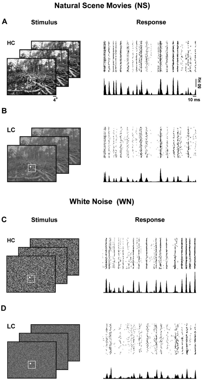
A) Typical frames of the high contrast natural scene movie stimulus and the responses of an ON-center X cell to repeated presentations of a short stimulus segment. The region of the frame that was presented during the experiment is denoted by the white box (10° × 10°). The spatial extent of the RF of the cell for which responses are shown is denoted by the white circle. B–D) Typical frames and responses of the same cell for the low contrast natural scene movie stimulus, and the high and low contrast spatiotemporal white noise stimuli.
We designed the stimuli to allow a systematic study of adaptation to changes in stimulus contrast and correlations. To examine the effects of a change in stimulus contrast, we compared responses to the HC and LC versions of each stimulus, as they were identical aside from the difference in contrast. To examine the effects of a change in stimulus correlations, we compared responses during stimulation with low contrast NS (strong spatiotemporal correlations) and low contrast WN (no spatiotemporal correlations), as the mean firing rates for these stimuli across the sample of 31 cells were not significantly different (paired t tests, p > 0.2).
To characterize the effects of changes in stimulus contrast and correlations on the functional properties of LGN neurons, we fit the components of an LN model from responses to each of the four stimuli. The LN model consists of a linear spatiotemporal RF followed by a static NL, as shown in Figure 2A. To estimate RFs, a least-squares technique was used which accounted for the correlations in the natural stimuli and prevented them from biasing the RF estimate (see Experimental Procedures). To estimate NLs, the stimulus was convolved with the estimated RF (after normalizing the RF to have unit variance) and the resulting filtered stimulus was compared to the actual firing rate response. Across the sample of 26 cells for which we recorded responses to repeated identical segments of the HC and LC natural stimuli for crossvalidation, the LN model provided accurate predictions of the LGN responses to novel natural stimuli, with correlation coefficients of 0.7 ± 0.07 for HC and 0.76 ± 0.07 for LC (for firing rate in 8 ms bins).
Figure 2. LGN cells adapt to changes in stimulus contrast and correlations.
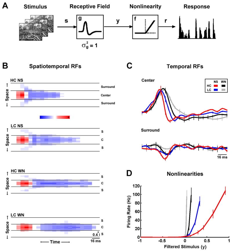
A) A linear-nonlinear model of encoding in the early visual pathway. The spatiotemporal visual stimulus (s) is passed through a linear filter (g, the spatiotemporal RF) to produce the filtered stimulus (y). The filtered stimulus is then passed through a rectifying static nonlinearity (f) to produce a nonnegative firing rate response (r). The RF is normalized to have unit variance. B) The spatiotemporal receptive fields for a typical cell (ON-center X) during high and low contrast natural scene movie and white noise stimulation. The full spatiotemporal RF was averaged radially to collapse space to one dimension. Regions where an increase in light intensity is excitatory are colored red and regions where an increase in light intensity is inhibitory are colored blue. Center and surround regions are separated by solid black lines. C) The temporal profiles extracted from the spatiotemporal RFs in B, averaged over all pixels in the center and surround. The error bars indicate ± one standard deviation of the RF estimates from 9 separate stimulus segments. D) The nonlinearities for the same cell during high and low contrast natural scene movie and white noise stimulation. The error bars indicate ± one standard deviation of the NL estimates from 9 separate stimulus segments.
The RFs and NLs of a typical cell as estimated from responses to the four stimuli are shown in Figures 2B–D. Figure 2B shows the spatiotemporal RFs (note that because the RFs are radially symmetric, space has been collapsed to a single dimension for plotting). There are clear differences evident in both the spatial and temporal properties of the RFs across stimuli. For example, a comparison of the high contrast natural scene RF (HC NS, top) with the low contrast white noise RF (LC WN, bottom) shows a change in the relative strength of the surround, and well as in the temporal dynamics. These changes are also evident in the temporal profiles of the RF center and surround, as shown in Figure 2C. The temporal profile of the high contrast natural scene RF (red) shows the strongest surround and fastest temporal dynamics, while the temporal profile of the low contrast white noise RF (gray) shows the weakest surround and the slowest temporal dynamics.
The effects of changes in stimulus contrast and correlations are also evident in the NLs of the cell, as shown in Figure 2D. For all stimuli, the NLs resemble half-wave rectifiers, producing zero output for negative inputs and positive output for positive inputs. However, there are also clear differences in the gain (slope) of the NLs for large positive inputs, as well is in the offset (the input required to evoke a non-zero response). For example, the gain of the low contrast white noise NL (gray) is the largest, while its offset is the smallest. Note that although the offset of the NL can be viewed as a threshold, we refer to it as an offset to avoid confusion with the physiological spike generation threshold.
To quantify the effects of changes in stimulus contrast and correlations on the functional properties of LGN neurons, we measured several properties of the RFs and NLs and compared the results across different stimulus conditions. To quantify changes in RFs, we measured the width of the spatial RF center, the relative strength of the surround and the width of the temporal profile of the RF center, as illustrated in Figure 3A. Across the sample of 68 cells for which we recorded responses to HC and LC natural stimuli, and the subset of 31 cells for which we also recorded responses to HC and LC white noise stimuli, decreases in contrast had no significant effect on the width of the spatial RF, as shown in Figure 3B. However, across the sample of 31 cells for which we recorded responses to both NS and WN stimuli, a decrease in correlations caused an average decrease of 20% in the width of the spatial RF center.
Figure 3. Adaptation of receptive fields to changes in stimulus contrast and correlations.
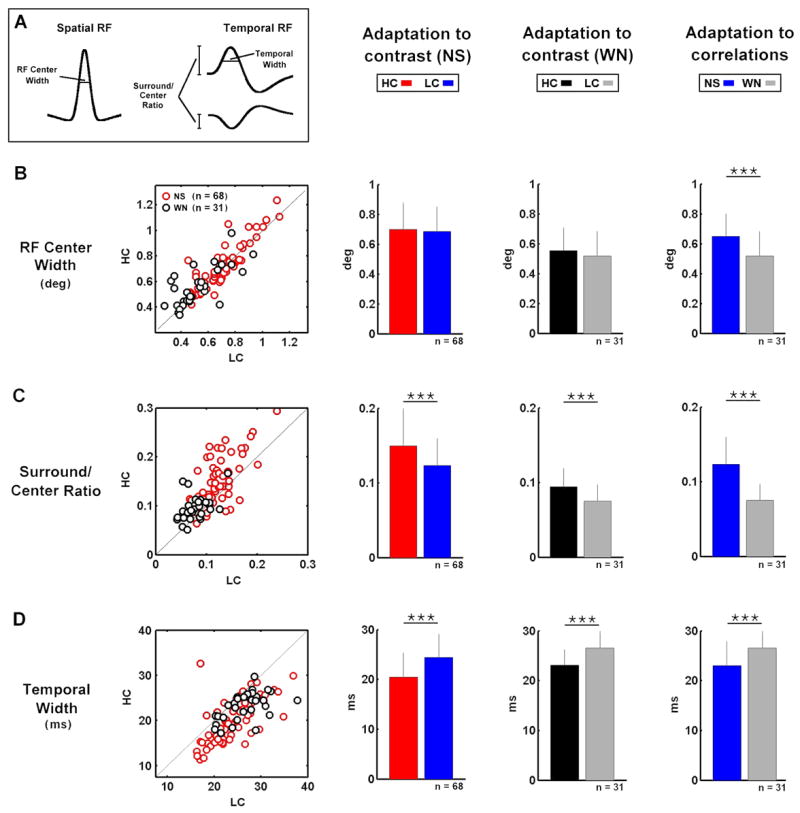
A) A schematic diagram defining the measured receptive field properties: RF center width is the width of the spatial RF center at half of its maximum value (at the peak latency), surround/center ratio is the ratio of the peaks of the temporal profiles of the RF surround and center, temporal width is the width of the primary phase of the temporal profile of the RF center at half of its maximum value. Further detail is given in the Experimental Procedures. B) The widths of the spatial RF center during high and low contrast natural scene movie and white noise stimulation for a sample of LGN cells. Bar plots show the sample averages and error bars represent one standard deviation. Significant differences (based on paired t tests) are marked by asterisks (*** denotes p < 0.001). C,D) The surround/center ratios and temporal widths during high and low contrast natural scene movie and white noise stimulation for a sample of LGN cells.
Both the relative strength of the surround and the width of the temporal pro- file of the RF center adapted to changes in both contrast and correlations, as shown in Figures 3C–D. The relative strength of the surround was decreased by a decrease in contrast during both NS (17%) and WN (18%) stimulation, as well as by a decrease in correlations (34%), while the width of the temporal profile of the RF center was increased by a decrease in contrast during both NS (16%) and WN (15%) stimulation, as well as by a decrease in correlations (15%). These contrast- and correlation-induced changes in spatial and temporal RF properties were correlated. For example, the correlation coefficient between the relative strength of the surround and the width of the temporal profile of the RF center during HC and LC natural stimulation was −0.5 (p < 0.001). The correlations between all changes in RF and NL properties are shown in Supplementary Figure 1.
To quantify changes in NLs, we measured the gain (α) and offset (θ) as illustrated in Figure 4A. The gain adapted to changes in both contrast and correlations. The gain was increased by a decrease in contrast during both NS (89%) and WN (148%) stimulation, as well as by a decrease in correlations (296%), as shown in Figure 4B. The offset adapted to a change in contrast, but not to a change in correlations. As shown in Figure 4C, the offset was decreased by a decrease in contrast during both NS (56%) and WN (59%) stimulation, but a decrease in correlations had no effect.
Figure 4. Adaptation of nonlinearities to changes in stimulus contrast and correlations.
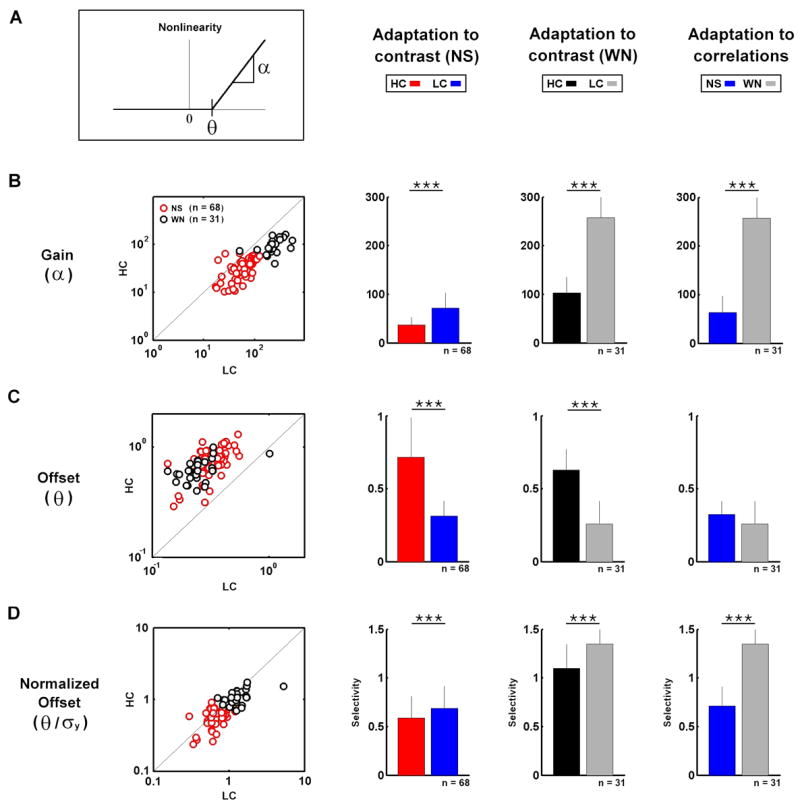
A) A schematic diagram defining the measured nonlinearity properties: Gain (α) is the slope of the nonlinearity for large inputs, offset (θ) is the input required to evoke a non-zero response. Further detail is given in the Experimental Procedures. B) The gains during high and low contrast natural scene movie and white noise stimulation for a sample of LGN cells. Bar plots show the sample averages and error bars represent one standard deviation. Significant differences (based on paired t tests) are marked by asterisks (*** denotes p < 0.001). C–D) The offsets and normalized offsets (selectivity) during high and low contrast natural scene movie and white noise stimulation for a sample of LGN cells.
Since the stimuli have different contrasts and the RFs are normalized to have unit variance, the sizes of the filtered stimuli (the inputs to the NLs) will vary. Because of these variations, the value of offset is only meaningful relative to the size of the corresponding filtered stimulus. Thus, rather than specify the absolute value of the offset, it is more informative to normalize it, giving a value for the neuron’s selectivity relative to the standard deviation of the filtered stimulus. Comparing the normalized offsets across stimulus conditions reveals changes that are quite different from those observed for the absolute offsets shown in Figure 4C. As shown in Figure 4D, the normalized offset was increased by a decrease in contrast during both NS (14%) and WN (24%) stimulation, as well as by a decrease in correlations (90%).
The above results rely on steady-state responses to stimuli with different contrasts and correlations. However, under truly natural conditions, the statistics of the visual stimulus can vary over time. To verify that the changes in the functional properties of LGN neurons described above are also observable under conditions where the stimulus contrast changes dynamically, we investigated whether similar changes in RFs and NLs were evident within a single presentation of the high contrast NS stimulus. Figure 5A shows the contrast within the spatial RF of a cell as it varies over time during a segment of the HC movie, reaching values as high as 0.43 and as low as 0.27.
Figure 5. Contrast adaptation during a single stimulus trial.
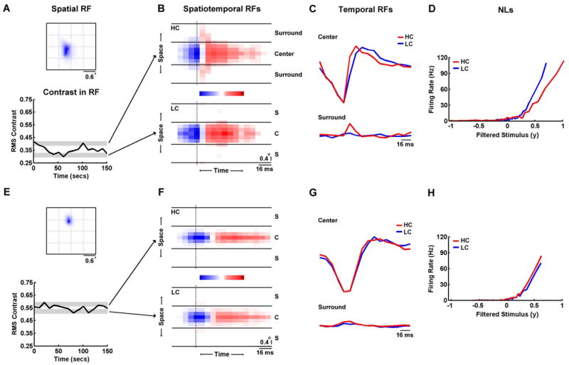
A) The spatial receptive field and the temporal contrast averaged over the spatial RF for an OFF-center Y cell during a 150 s segment of the high contrast movie. The gray bars denote the top and bottom third of all contrast values during the entire movie. B) The spatiotemporal RFs during movie segments with contrast in the top (HC) and bottom (LC) third of all values for the cell shown in A, displayed as in Figure 2A. C) The temporal profiles of the RF center and surround extracted from the spatiotemporal RFs in B. D) The static nonlinearities during movie segments with contrast in the top (HC) and bottom (LC) third of all values for the cell shown in A. E–H) Results for an OFF-center X cell, displayed as in A–D.
We estimated separate RFs and NLs for those periods during which the contrast within the RF was within either the top or bottom third of all values for this cell (denoted by the gray bands). As shown in Figures 5B–D, the changes evident in the surround strength and temporal dynamics of the RF, and gain and offset of the NL are similar to those described above. For a second cell with its RF in a different location within the visual stimulus, the contrast is much higher and varies over a smaller range, as shown in 5E. As shown in Figures 5F–H, the RFs and NLs estimated from the highest and lowest contrast periods of the stimulus for this cell are nearly identical. These examples suggest that the characterization of the effects of changes in stimulus contrast and correlations on the functional properties of LGN neurons achieved through our analysis of steady-state responses to HC and LC natural and white noise stimuli may also be applicable under more dynamic natural conditions.
Contrast- and correlation-induced changes in the reliability and sparseness of LGN responses
The results described in the previous section provide a characterization of the functional properties of LGN neurons within the LN framework. Through further examination of these results, we can relate these functional properties to contrast- and correlation-induced changes in the LGN responses. To quantify the effects of changes in stimulus contrast and correlations on LGN responses, we measured the reliability and sparseness of responses to repeated identical stimuli and compared the results across different stimulus conditions. We de- fined reliability as the signal to noise ratio for firing rate responses in 8 ms bins, and we measured sparseness on a scale from 0 to 1, with 0 corresponding to a response that is the same during every bin, and 1 corresponding to a response that is non-zero only in a single bin (see Experimental Procedures).
Across the sample of 31 cells from which we recorded responses to all four stimuli, a decrease in contrast during natural stimulation caused an average decrease of 54% in reliability, as shown in Figure 6A. Similar decreases in reliability were caused by a decrease in contrast during white noise stimulation (74%), and by a decrease in correlations (68%). As shown in Figure 6B, a decrease in contrast during natural stimulation caused only a small decrease in sparseness (4%), but larger decreases in sparseness were evident for a decrease in contrast during white noise stimulation (16%), and for a decrease in correlations (14%).
Figure 6. The reliability and sparseness of LGN responses to natural scene movie and white noise stimuli.
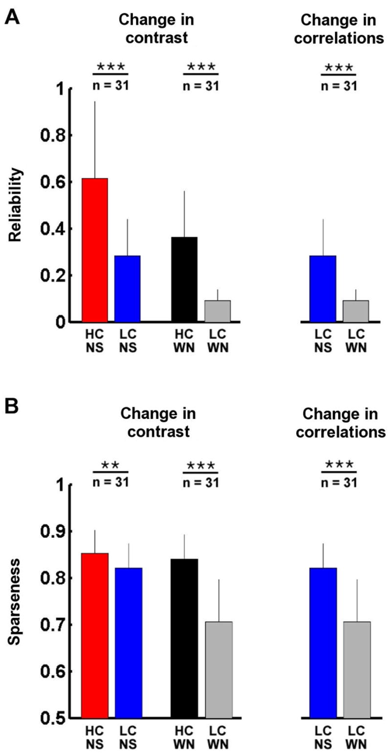
A) Reliability of responses across a sample of LGN cells during high and low contrast natural scene movie and white noise stimulation. Error bars represent one standard deviation. Reliability was calculated as signal to noise ratio for firing rate in 8 ms bins (see Experimental Procedures). Significant differences (based on paired t tests) are marked by asterisks (** denotes p < 0.01, *** denotes p < 0.001). B) Sparseness of LGN responses, displayed as in A. Sparseness was calculated as described in the Experimental Procedures.
To relate the functional properties of LGN neurons to these contrast- and correlation-induced changes in reliability and sparseness, we created a generic LN model for each of the four stimuli. The RFs for each model were obtained by averaging the estimated RFs across the sample of cells (with a sign reversal for OFF-center cells). The average RFs, shown in Figure 7A, display the same adaptive effects that were evident in the single cell example shown in Figure 2. NLs for each model were perfect half-wave rectifiers (zero output for inputs that were less than the offset, linear output for inputs that were greater than the offset), with gains and offsets determined by the average values across the sample of cells (see below in Figure 8A). Using the generic models, we can simulate the firing rate response to each stimulus and relate the processing that takes place in the RFs and NLs to reliability and sparseness.
Figure 7. Effective contrast determines the reliability of LGN responses.
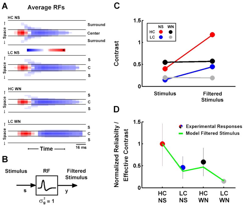
A) The spatiotemporal receptive fields for high and low contrast natural scene movie and white noise stimuli averaged across a sample of LGN cells. RFs for OFF-center cells were sign-reversed before averaging. RFs are displayed as in Figure 2A. B) The linear part of the linear-nonlinear model of encoding in the early visual pathway. The spatiotemporal visual stimulus (s) is passed through a linear filter (the spatiotemporal RF) to produce the filtered stimulus (y). The RF is normalized to have unit variance. C) The RMS contrast of the high and low contrast natural scene movie and white noise stimuli, and the corresponding ‘effective contrast’ of the filtered stimuli after processing in the RFs shown in A. D) The average reliability of experimental LGN responses to high and low contrast natural scene movie and white noise stimuli (circles, error bars represent one standard deviation) and the corresponding effective contrasts of filtered high and low contrast natural scene movie and white noise stimuli (line). Both sets of values were normalized to their values during high contrast natural scene stimulation.
Figure 8. Stimulus sparseness, effective contrast, noise, and offset determine the sparseness of LGN responses.
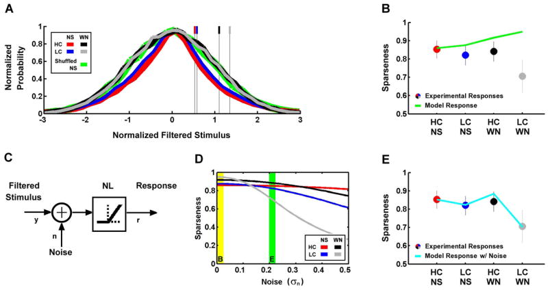
A) The probability distributions of filtered high and low contrast natural scene movie and white noise stimuli after processing in the RFs shown in Figure 7A (thick lines), and the corresponding normalized offsets (thin lines). The result of shuffling the frames of the high contrast NS stimulus before filtering is also shown. Distributions were normalized to have unit standard deviation and the same peak value. B) The average sparseness of experimental LGN responses to high and low contrast natural scene movie and white noise stimuli (circles, error bars represent one standard deviation) and corresponding sparseness of LN model responses (line). C) The nonlinear part of the linear-nonlinear model of encoding in the early visual pathway with added noise. The filtered stimulus (y) is added to Gaussian white noise (n) before passing through the static nonlinearity to produce the response (r). D) The sparseness of LN model responses to high and low contrast natural scene movie and white noise stimuli for different levels of noise. The yellow bar indicates no noise, as shown in B, and the green bar indicates the noise level where sparseness of the model responses matches that observed experimentally, as shown in E. E) The average sparseness of experimental LGN responses to high and low contrast natural scene movie and white noise stimuli (circles, error bars represent one standard deviation) and corresponding sparseness of LN model responses (line) with the noise level marked by the green bar in D.
We examined the effects of spatiotemporal integration under each stimulus condition by comparing the contrast of the stimulus before and after processing in the RF, as illustrated in Figure 7B. Figure 7C shows the RMS contrast (standard deviation) of the four stimuli along with the standard deviation of the corresponding filtered stimuli, which we denote ‘effective contrast’. Because the RFs are normalized to have unit variance, the difference between the original and effective contrasts is a direct measure of the extent to which a stimulus contains the features to which the corresponding RF is sensitive. As is evident in Figure 7C, spatiotemporal integration in the RF results in an increase in the effective contrasts of the NS stimuli relative to those of the WN stimuli, indicating that the NS stimuli contain more of the features to which the RF is sensitive. As shown in Figure 7D, a comparison of the effective contrasts of the four stimuli (line) with the experimentally observed reliability in the LGN responses (circles) reveals a strong correspondence (note that, because of the difference in the units of reliability and effective contrast, both sets of values are normalized to their values for high contrast NS). This suggests that it is not the overall contrast of the stimulus, but its effective contrast that determines the reliability of LGN responses.
To understand the contrast- and correlation-induced changes in the sparseness of LGN responses, we must consider both the properties of the filtered stimulus as well as the additional processing that takes place in the NL. Figure 8A shows the probability distributions of the stimuli after filtering in the generic RFs (thick lines), normalized to have unit standard deviation and the same peak value, along with the corresponding normalized offsets of the generic NLs (thin lines). The distributions of the filtered NS stimuli (red and blue) have relatively heavy tails (and, therefore, high sparseness), indicated by a high kurtosis (k = 4.06), while those of the filtered WN stimuli (black and gray) are Gaussian (k = 3.01). The high kurtosis in the distributions of the filtered NS stimuli disappears when the frames of the stimuli are shuffled before spatiotemporal integration in the RF (green), indicating that the increased kurtosis is due primarily to the temporal correlations in the NS. The kurtosis of the filtered stimulus affects the sparseness of the overall response, as the sparseness of the response of the generic LN model (with high contrast natural scene RF and NL) to the original high contrast NS stimulus is 0.86 and shuffling the frames of the stimulus decreases this value to 0.83.
Sparseness is also dependent on the offset of the NL, as only those filtered stimuli which are greater than the offset can evoke a response. Thus, one expects the sparseness of the model responses to increase as the normalized offset is increased, with the lowest sparseness for high contrast NS responses and the highest sparseness for low contrast WN responses. Indeed, as shown in Figure 8B, the sparseness of the model responses (line) increases as contrast and correlations are decreased. However, this is the opposite of what is observed in the experimental responses (circles), where decreases in contrast and correlations evoke a decrease in sparseness. While the sparseness of the model responses to high contrast NS stimuli matches that observed experimentally, the correspondence between model and experiment for low contrast WN is relatively weak.
The differences in the sparseness of the model and experimental responses shown in Figure 8B can be reconciled by adding noise to the filtered stimulus in the LN model, as illustrated in Figure 8C. This added noise increases the variability of responses to identical stimuli and, therefore, decreases the sparseness of the response. Because the filtered stimuli have different effective contrasts, a fixed level of noise will have a different effect on each stimulus, causing a relatively small decrease in the sparseness of the high contrast NS response and a relatively large decrease in the sparseness of the low contrast WN response. As shown in Figure 8D, as the noise level is increased, the sparseness of the model responses is decreased, with the strongest decreases for the low contrast WN responses. When there is no noise (figure 8D, yellow bar), the sparseness is highest for the low contrast WN response and lowest for the high contrast NS response, as was shown in Figure 8B (green line). As the noise level is increased and the sparseness of the responses decrease at different rates, there is a certain noise level (figure 8D, green bar) at which the sparseness of the model and experimental responses are in close agreement, as shown in Figure 8E. These results suggests that the sparseness of LGN responses is determined by a number of factors, including the sparseness and effective contrast of the filtered stimulus, noise, and the offset of the NL.
Discussion
By comparing responses to high and low contrast natural scene movie and white noise stimuli, we have shown that the functional properties of LGN neurons adapt to changes in stimulus contrast and correlations. In response to a decrease in contrast, we observed changes in spatiotemporal integration, evidenced by an decrease in the surround strength and a slowing of the temporal dynamics of the RF. A decrease in contrast also evoked increases in gain (a given stimulus caused a larger response) and selectivity (a larger stimulus was required to evoke a response), evidenced by increases in the gain and normalized offset of the NL. A decrease in correlations evoked similar changes, as well as a decrease in the spatial extent of the RF center. These results reveal a number of novel adaptive phenomena and provide a comprehensive characterization of the effects of changes in stimulus contrast and correlations on LGN response properties.
Relation to previous studies of contrast adaptation
Our results regarding the effects of contrast adaptation on temporal dynamics, gain, and offset are consistent with those of previous studies in the early visual pathway. The first studies of contrast adaptation in the retina reported changes in gain and temporal dynamics similar to those observed in our results (Shapley and Victor, 1978, 1981). As the contrast of a grating stimulus was increased, the temporal frequency responses of retinal ganglion cells showed a decrease in overall gain, a phase advance, and a shift in tuning toward higher temporal frequencies (corresponding to the decrease in gain and transition to faster dynamics in our results). These changes were well predicted by a model in which ganglion cell dynamics were dependent on a measure of ‘neural contrast’ similar to the measure of effective contrast used here (Victor, 1987). More recent studies using white noise stimuli and LN model-based analyses have reported similar changes (Smirnakis et al., 1997; Chander and Chichilnisky, 2001; Kim and Rieke, 2001; Brown and Masland, 2001). Studies of contrast adaptation in the retina using intracellular recordings have also reported changes in baseline membrane potential (Baccus and Meister, 2002; Zaghloul et al., 2005). Following an increase in the contrast of the stimulus, the steady-state baseline membrane potential of retinal ganglion cells decreased (corresponding to the increase in normalized offset in our results). Recent studies in the LGN have used gratings of different contrasts to demonstrate similar effects on gain and temporal dynamics (Mante et al., 2005), as well as baseline membrane potential (Solomon et al., 2004). Our results verify that these changes in temporal dynamics, gain, and offset are also evident under more natural stimulus conditions.
It is likely that the adaptive changes that we observe in the LGN originate in the retina. Contrast-induced changes in temporal dynamics, gain, and offset are already evident in bipolar cells (Kim and Rieke, 2001; Rieke, 2001; Manookin and Demb, 2006; Beaudoin et al., 2007) and are enhanced during spike generation in ganglion cells (Kim and Rieke, 2001; Zaghloul et al., 2005; Beaudoin et al., 2007). The mechanisms that underlie these changes are activity dependent (Rieke, 2001; Kim and Rieke, 2003; Manookin and Demb, 2006; Beaudoin et al., 2007), suggesting that the level of adaptation is determined by the effective contrast of stimulus (not the RMS contrast), which is consistent with our results.
Our results also demonstrate that an increase in contrast during both natural and white noise stimulation causes an increase in the strength of the RF surround and has no effect on the size of the RF center. There have been several studies of the effects of stimulus contrast on the spatial RFs of LGN neurons using disk and grating stimuli, but explicit comparison of our results with those of these studies is difficult. One study using concentric disks to stimulate the center and surround separately found that increasing the contrast of the surround stimulus caused an increase in surround strength (Kremers et al., 2004), which is consistent with our results. Another study using disk stimuli reported a change in the size of the RF center, but no change in the relative strength of the classical RF surround (Nolt et al., 2004). However, the stimuli used in this study were spatially uniform (only the temporal contrast was changed), and it is possible that the changes in surround strength that we observe are due to changes in spatial contrast that were not present in the disk stimulus. Finally, a recent study using grating stimuli reported that an increase in contrast caused an increase in the strength of the ‘suppressive field’ (Bonin et al., 2005). Any differences between our results and the results of these studies are likely due to the properties of the stimuli used in each study, but further study is necessary to fully clarify this issue.
Relation to previous studies of adaptation to correlations
To our knowledge, there is only one other study in the early visual pathway with which to compare our results on adaptation to stimulus correlations. Hosoya and colleagues (2005) showed that the RFs of retinal ganglion cells adapt to predictable spatial and temporal patterns in a manner that facilitates the detection of novel stimuli. These results are consistent with our observations of the differences in the RFs estimated from responses to natural and white noise stimuli at the same contrast. For example, natural stimuli contain strong spatial correlations and the increased strength of the RF surround during natural stimulation decreases the sensitivity of the neuron to these correlations while increasing its sensitivity to novel stimuli such as edges. This interpretation is also consistent with the results of a recent study in the visual cortex which demonstrated that changes in spatial frequency tuning evoked by changes in stimulus correlations increase the information in the neural response (Sharpee et al., 2006). We also observed differences in the gains and normalized offsets of the NLs estimated from responses to NS and WN stimuli at the same overall contrast, but as of yet there are no comparable studies of these phenomena.
The effects of contrast and correlations on reliability and sparseness
Our results suggest that the reliability and sparseness of LGN responses are determined not by the overall contrast of the stimulus, but by its effective contrast (the standard deviation of the stimulus after filtering in the RF). Effective contrast is a direct measure of the extent to which a stimulus contains the features to which the RF is sensitive, and is similar to other measures of local contrast that have been used previously (Victor, 1987; Tadmor and Tolhurst, 2000). Effective contrast can be viewed in the frequency domain as the extent to which the frequency content of the stimulus and the frequency tuning of the neuron overlap. From this perspective, it is apparent why the effective contrast of NS stimuli is higher than that of WN stimuli with a similar overall contrast (see Figure 7C), as the power in NS stimuli is concentrated at low frequencies to which the system is most sensitive, while power in WN stimuli is spread evenly across all frequencies.
In examining the effects of stimulus correlations on LGN responses, we chose to compare low contrast NS and WN responses because these stimuli had similar RMS contrasts and evoked responses with similar mean firing rates. However, because these stimuli also have different effective contrasts, it is possible that the observed differences in the reliability and sparseness of low contrast NS and WN responses are not due to the change in correlations per se, but instead to the change in effective contrast that results from the change in correlations. If this were true, then the reliability and sparseness of responses to low contrast NS and high contrast WN, which have different correlations but similar effective contrasts, should be similar. Indeed, when comparing responses to low contrast NS and high contrast WN stimuli, the decreases in reliability and sparseness corresponding to the decrease in correlations are no longer evident (see Figures 6A and B). In fact, the reliability and sparseness of the high contrast WN responses are slightly higher than those of the low contrast NS responses. This suggests that, while stimulus correlations have an indirect effect on reliability and sparseness, these response properties are determined primarily by effective contrast.
Adaptation to stimulus correlations
Given that it is not correlations themselves, but their impact on the effective contrast of the stimulus that underlies the differences in the reliability and sparseness of low contrast NS and WN responses, one might also expect that the adaptive changes evident in the comparison of the low contrast natural scene and white noise RFs and NLs are also driven by the change in effective contrast, not the change in correlations. If this were true, then these changes, like those in reliability and sparseness, would no longer be evident in a comparison between the RFs and NLs for NS and WN stimuli with similar effective contrasts. However, nearly all of the observed differences between low contrast natural scene and white noise RFs and NLs (spatial width, surround strength, gain, and normalized offset) are still significant when RFs and NLs are compared across low contrast NS and high contrast WN. This suggests that these effects are indeed adaptations to stimulus correlations, as they are evident when the natural scene and white noise RFs and NLs are compared at similar overall and effective contrasts. Thus, while reliability and sparseness are similar for stimuli with different correlations (and similar effective contrasts), the underlying RFs and NLs are different, indicating that the observed changes in RFs and NLs reflect adaptive mechanisms designed to preserve reliability and sparseness.
The functional mechanisms underlying reliability and sparseness
Our results suggest that reliability is dependent primarily on the effective contrast of the stimulus (see Figure 7), while sparseness is determined by a number of factors including the sparseness and effective contrast of the filtered stimulus, noise, and the offset of the NL (see Figure 8). Because filtered NS stimuli are more sparse than filtered WN stimuli (as measured by kurtosis), responses to NS (with a fixed NL) will be more sparse than responses to WN at the same effective contrast. Sparseness is also influenced by the relative sizes of the stimulus-dependent neural activity (effective contrast) and the stimulus-independent neural activity (noise). For stimuli with a high effective contrast, the neuron will respond reliably to the features of the stimulus to which it is sensitive, with high sparseness (constrained by the sparseness of the stimulus). For stimuli with a low effective contrast, the response of the neuron will be a maintained discharge driven primarily by noise, with equal probability of response at all times and, thus, low sparseness. Our data suggest that the offset of the NL adapts to changes in stimulus sparseness (as determined by correlations) and effective contrast to maintain the sparseness of the response. For example, the offsets for low contrast NS and high contrast WN (stimuli with different sparseness and similar effective contrast) are dramatically different while the sparseness of LGN responses to these stimuli are similar.
The coding of natural stimuli in the LGN
Our results show that natural stimuli are coded with greater reliability and sparseness than white noise stimuli in the LGN, and suggest that these differences are due to differences in effective contrast. For stimuli with similar overall contrasts, the reliability and sparseness of responses to natural stimuli were higher than those of responses to white noise (see Figures 6A and B). Furthermore, the sparseness of LGN responses was far more robust to a change in contrast during natural stimulation than during white noise stimulation. While a decrease in contrast caused a small decrease in sparseness during natural stimulation, the decrease was much larger during white noise stimulation. Thus, the mechanisms that produce a sparse response in the LGN may be effective over the range of effective contrasts that are typical during natural stimulation, but are unable to maintain sparseness at the very low effective contrast of the low contrast WN stimulus. This suggests that the adaptive changes that we have characterized here may be optimized for the processing of visual stimuli with statistical properties that are typical of the natural environment.
Experimental Procedures
Recordings from cat LGN
The surgical and experimental preparations used for this study have been described in detail previously (Weng et al., 2005). Briefly, cats were initially anesthetized with Ketamine (10 mg/kg, intramuscular) followed by thiopental sodium (surgery: 20 mg/Kg, intravenous; recording: 1–2 mg/Kg/hr, intravenous; supplemented as needed). A craniotomy and duratomy were made to introduce recording electrodes into LGN (anterior: 5.5; lateral 10.5). Animals were paralyzed with Atracurium Besylate (0.6–1 mg/kg/hr, intravenous) to minimize eye movements and artificially ventilated. All surgical and experimental procedures were performed in accordance with United States Department of Agriculture (USDA) guidelines and were approved by the Institutional Animal Care and Use Committee (IACUC) at the State University of New York, State College of Optometry. LGN responses were recorded extracellularly within layer A. Recorded voltage signals were conventionally amplified, filtered, and passed to a computer running the RASPUTIN software package (Plexon Inc., Dallas, TX). For each cell, spike waveforms were identified initially during the experiment and verified carefully off-line by spike sorting analysis. Cells were classified as X or Y according to their responses to counterphased sine wave gratings (Hochstein and Shapley, 1976). All cells included in this study were non-lagged cells.
Natural scene movie and white-noise stimuli
Movie sequences were recorded by members of the laboratory of Peter König (Institute of Neuroinformatics, ETH/UNI Zürich) using a removable lightweight CCD-camera mounted to the head of a freely roaming cat in natural environments such as grassland and forest (Kayser et al., 2003). It is important to note that while these movies provide an approximation of the actual stimulus that the cat receives in the natural environment, they do not capture the effects of saccades and fixational eye movements, which can have significant effects on the statistics of the visual input (Rucci and Casile, 2005). Movies were recorded via a cable connected to the leash onto a standard VHS-VCR (Pal) carried by the human experimenter and digitized at a temporal resolution of 25 Hz. Each frame of the movies consisted of 320 × 240 pixels and 16 bit color depth. For this study, the movies were converted to 8-bit gray scale and a 48 × 48 section of each frame was used. To improve temporal resolution, movies were interpolated by a factor of 2 (to a sampling rate of 50 Hz) using commercial software (MotionPerfect, Dynapel Systems Inc.). Following interpolation, the intensities of each movie frame were rescaled to have a mean value of 125 (possible values were 0–255) for presentation. For all analyses in this study, the stimuli were scaled to have zero mean and possible values between −106 and 106. To create high and low contrast versions of the movies, each frame was rescaled to have an RMS contrast of 0.40 (high contrast) or 0.15 (low contrast). Aside from the difference in contrast, the high and low contrast movie segments were identical, and the contrast transformations did not affect the mean intensity of the stimulus. Thus, within the RF of any particular neuron, the mean intensity of the high and low contrast movies was the same. During experimental presentation, movies were shown on a 20-inch monitor with a refresh rate of 120 Hz, with pixel intensities updated every other refresh so that playback approximated the intended temporal resolution of the interpolated movies. The spatial resolution of the stimulus was such that each pixel was a square measuring 0.2° (RF center width, when measured as described below, was typically between 0.5 – 0.7°).
For all cells in this study, a single 15 min movie segment was shown at high and low contrast for RF and NL estimation. For analysis of the single 15 min movie segments, only those cells for which the peak of the RF estimate was at least 10 times larger than the noise (standard deviation of RF estimated from shuffled responses) were included. This sample included 68 cells: 44 cells that were ON-center (19 X cells, 19 Y cells, and 6 cells that were not classified because responses to counterphased sine wave gratings were not recorded) and 24 cells that were OFF-center (11 X cells, 8 Y cells, and 5 cells that were not classified). For a subset of 26 cells, 24 repeated trials of a different 90 s movie segment were also shown at high and low contrast for cross-validation of the RFs and NLs. For a subset of 31 cells, a 6 min segment of a spatiotemporal binary white noise stimulus was also shown at high and low contrast, along with 120 repeated trials of different 12 s segments of natural scene movie and white noise stimuli at high and low contrast. For the white noise stimulus, each frame was rescaled to have an RMS contrast of 0.55 (high contrast) or 0.20 (low contrast). The spatial resolution and refresh rate of the white noise stimulus were the same as those of the movies.
Measurement of reliability and sparseness
Reliability and sparseness were measured from responses to repeated identical stimuli. Reliability was measured as the signal to noise ratio (for firing rate in 8 ms bins) as described by Borst and Theunissen (Borst and Theunissen, 1999). First, the signal spectrum is obtained by computing the power spectrum of the response after averaging across all trials. Next, to obtain the noise power, the response from each trial is subtracted from the average response and the power spectrum of this difference is computed. These difference spectra are averaged over all trials to yield the overall noise spectrum. Finally, the signal to noise ratio is given by the ratio of the total power of the signal and noise spectra.
Sparseness was measured as defined by Vinje and Gallant (Vinje and Gallant, 2000):
where μ is the mean firing rate, σ is the standard deviation of the firing rate, and n is the number of time bins. For a response that is the same in every time bin (flat PSTH), the sparseness is 0. For a response that is zero in all but one time bin, the sparseness is 1.
Estimation of receptive fields
In order to estimate receptive fields from responses to correlated natural stimuli, an estimation procedure which accounts for the auto-correlation structure of the stimulus must be employed. We have previously developed a recursive least-squares (RLS) algorithm to estimate RFs from responses to natural scene movies (Lesica and Stanley, 2006). Importantly, through recursive computation, RLS avoids the explicit inversion of the stimulus auto-correlation matrix, resulting in a convergence rate that is independent of the eigenvalue spread of the stimulus auto-correlation matrix (Haykin, 2002). This is especially important when estimating RFs from a limited presentation of correlated stimuli.
We denote the visual input as the spatiotemporal signal s[p, n]. For our computer driven stimuli discretized in space-time, p represents the grid index of a stimulus pixel on the screen and n is the time sample. We denote the RF as g[p,m], representing P (total pixels in stimulus) separate temporal RFs, each with M (length of temporal RF) lags. To generate a linear prediction of the LGN response, the stimulus is convolved with the RF: y[n] = sn * gn, If s and g are organized appropriately into the column vectors sn and gn, then this discrete time integration in space and convolution in time can be written as a vector multiplication y[n] = snTgn, where sn and gn are the column vectors:
and T denotes matrix transpose. At each time step, the RF estimate computed from previous data ĝn|n−1 is used to generate a linear prediction of the response of the neuron to the new stimulus (the subscript n|n − 1 denotes an estimate at time n given all data up to and including time n − 1). This prediction is compared with the actual response r[n] to yield the prediction error: e[n] = r[n] − snT ĝn|n−1. The RF estimate is updated by scaling the error by a gain factor related to the correlation structure of the stimulus: ĝn+1|n = ĝn|n−1 + Gn e[n]. The gain is computed each time step as follows:
To initialize the algorithm, the initial conditions ĝ0|−1 = 0 and K 0|−1 = Δ × I are used. The regularization parameter Δ affects the convergence properties and steady state error of the RLS estimate. Estimating an RF using a least-squares method requires the inversion of the stimulus auto-correlation matrix (although in RLS, explicit inversion is avoided via recursive solution). If the stimulus is correlated, the eigenvalue spread of the auto-correlation matrix can become rather large, and the inversion may be ill-conditioned. Regularization of this matrix can reduce its condition number (ratio of largest to smallest eigenvalue) by adding a constant to all of the elements along the diagonal (Haykin, 2002). However, this manipulation of the diagonal elements of the stimulus auto-correlation matrix also introduces a bias into the RF estimate. Thus, regularization is a tradeoff between error avoided by decreasing the condition number of the stimulus auto-correlation matrix and error introduced by biasing the RF estimate. A set of rules for choosing this value based on the signal to noise ratio in the system has been developed (Haykin, 2002). For this study, the value of Δ which produced the RF estimates that provided the most accurate predictions of responses to natural scene movies was used (Δ = 0.001).
In addition to having strong spatial and temporal correlations, natural stimuli are often also spherically asymmetric (Simoncelli et al., 2003), and this asymmetry can bias RF estimates obtained using least-squares techniques such as the one described above. To examine the effects of spherical asymmetry in our RF estimates, we simulated LGN responses using the LN model with a known RF and NL as described below. We estimated the RF from simulated responses to both Gaussian white noise stimuli and the movie stimuli used in this study and found that the estimates were not significantly different, which suggests that the spherical asymmetry of the movies used in this study did not cause a large bias in the experimental RF estimates.
For RF estimation, spike times were binned at 128 Hz to give an estimate of the firing rate. Thus, each spatiotemporal RF estimate consisted of 441 spatial points (21 × 21 grid) spaced at 0.2 cycles per degree each with 24 temporal points spaced at 8 ms. RF estimates for a given cell were estimated using the same number of spikes for high and low contrast responses. Each response was broken into 9 segments and RFs were calculated separately for each segment. The mean of these 9 RFs was used for measuring RF properties and in the LN model to predict the response of the neuron to novel stimuli. The error bars on the RF estimates represent ± one standard deviation of the 9 RF estimates.
Definition of center and surround
RFs were separated into center and surround components using the following method (Lesica and Stanley, 2004): First, the point with the largest amplitude (maximal point) in the spatiotemporal RF was determined. Next, the center of the RF was defined as those spatial points at the same latency as the maximal point that 1) formed a contiguous region with the maximal point and other center pixels and 2) had an amplitude with the same sign as the maximal point and a value that was above the error level for that neuron. The error level for each neuron was based on the RF estimate from randomly shuffled responses. The standard deviation of this estimate (equal to zero in an ideal setting with infinite data) provides a measure of the uncertainty in the actual RF estimate. The surround was defined as a ring around the center region, a maximum of 4 pixels wide.
Estimation of static nonlinearities
The static nonlinearities for each cell were calculated by convolving the stimulus with the spatiotemporal RF to yield the filtered stimulus and comparing it with the actual response of the neuron (firing rate in 8 ms bins). Before convolution, the mean of each stimulus was set to zero and each RF was normalized to have unit variance. The values of the filtered stimulus were sorted into ascending order and separated into groups of 250 values. For each group, the mean values of the filtered stimulus and corresponding actual firing rates were used to define the static nonlinearity. As described above for the calculation of RFs, each response was broken into 9 segments and NLs were calculated separately for each segment. The mean of these 9 NLs was used for measuring NL properties and in the LN model to predict the response of the neuron to novel stimuli. The error bars on the NL estimates represent ± one standard deviation of the 9 NL estimates.
Measurement of receptive field and nonlinearity properties
To quantify the effects of adaptation to changes in stimulus contrast and correlations, we measured several properties of the estimated RFs and NLs. To measure the width of the spatial RF, the spatial profile of the RF (at the latency of the peak) was fit with a symmetric two-dimensional difference of Gaussians function. The width of the spatial RF was defined as the width of this function at half of its peak value. The surround/center ratio and temporal width of the RF were measured directly from the raw RF estimates. The sur- round/center ratio of the RF was defined as the absolute value of the peak of the temporal profile of the RF surround divided by the peak of the temporal profile of the RF center. The width of the temporal RF was defined as the width of the primary phase of the temporal profile of the RF center at half of its peak value. Changes in contrast and correlations also had significant effects on the latency (time to peak) of the temporal profile of the RF center, but not on the biphasic ratio (the absolute value of the peak of the primary phase of temporal profile of the RF center divided by the peak of the secondary phase of temporal profile of the RF center).
To measure gain (α) and offset (θ), the static nonlinearities were fit with a half-wave rectifier:
The only RF or NL parameter value that was significantly different across animals for a given stimulus condition was θ. This is likely due to the different anesthesia requirements of each animal, as θ is reflective of the baseline membrane potential (Baccus and Meister, 2002; Zaghloul et al., 2005). To account for this difference, the values of θ for each stimulus condition were adjusted to have the same mean value for each animal.
Across cell types (X/Y, ON/OFF), there were several significant differences between RF and NL parameters. The width of the spatial RF was significantly larger for Y cells than for X cells during both high contrast (X: 0.63 ± 0.16 deg., Y: 0.75 ± 0.18 deg.) and low contrast (X: 0.63 ± 0.14 deg., Y: 0.73 ± 0.15 deg.) natural stimulation (t tests, p < 0.01), the relative strength of the surround was significantly larger for Y cells than for X cells during high contrast natural stimulation (X: 0.13 ± 0.04, Y: 0.16 ± 0.06, t test, p < 0.05), and the width of the temporal profile of the RF center was significantly larger for OFF cells than for ON cells during low contrast white noise stimulation (ON: 25 ± 0.4 ms, OFF: 29 ± 0.4 ms, t test, p < 0.01). Also, the correlation coefficients between LN model predictions and experimental responses to repeated identical segments of novel NS stimuli (for firing rate in 8 ms bins) were higher for X cells than for Y cells at both HC (X: 0.73, Y: 0.69) and LC (X: 0.78, Y: 0.75), but these differences were not significant (t tests, p > 0.1).
Supplementary Material
Acknowledgments
NAL, DAB, and GBS were supported by National Geospatial-Intelligence Agency Grant HM1582-05-C-0009. JJ, CW, CIY, and JMA were supported by National Eye Institute Grant EY-05253 and Research foundation at State University of New York. The authors would like to thank C. Kayser and the members of the laboratory of Peter König for providing the natural scene movies, and C. Leibold and C. Machens for helpful discussions.
Footnotes
Publisher's Disclaimer: This is a PDF file of an unedited manuscript that has been accepted for publication. As a service to our customers we are providing this early version of the manuscript. The manuscript will undergo copyediting, typesetting, and review of the resulting proof before it is published in its final citable form. Please note that during the production process errors may be discovered which could affect the content, and all legal disclaimers that apply to the journal pertain.
References
- Baccus SA, Meister M. Fast and slow contrast adaptation in retinal circuitry. Neuron. 2002;36:909–919. doi: 10.1016/s0896-6273(02)01050-4. [DOI] [PubMed] [Google Scholar]
- Beaudoin DL, Borguis BG, Demb JB. Cellular basis for contrast gain control over the receptive field center of mammalian retinal ganglion cells. J Neurosci. 2007;27:2636–2645. doi: 10.1523/JNEUROSCI.4610-06.2007. [DOI] [PMC free article] [PubMed] [Google Scholar]
- Bonin V, Mante V, Carandini M. The suppressive field of neurons in lateral geniculate nucleus. J Neurosci. 2005;25:10844–10856. doi: 10.1523/JNEUROSCI.3562-05.2005. [DOI] [PMC free article] [PubMed] [Google Scholar]
- Borst A, Theunissen FE. Information theory and neural coding. Nat Neurosci. 1999;2:947–957. doi: 10.1038/14731. [DOI] [PubMed] [Google Scholar]
- Brenner N, Bialek W, de Ruyter van Steveninck R. Adaptive rescaling maximizes information transmission. Neuron. 2000;26:695–702. doi: 10.1016/s0896-6273(00)81205-2. [DOI] [PubMed] [Google Scholar]
- Brown SP, Masland RH. Spatial scale and cellular substrate of contrast adaptation by retinal ganglion cells. Nat Neurosci. 2001;4:44–51. doi: 10.1038/82888. [DOI] [PubMed] [Google Scholar]
- Chander D, Chichilnisky EJ. Adaptation to temporal contrast in primate and salamander retina. J Neurosci. 2001;21:9904–9916. doi: 10.1523/JNEUROSCI.21-24-09904.2001. [DOI] [PMC free article] [PubMed] [Google Scholar]
- Dong DW, Atick JJ. Statistics of time-varying images. Network: Comput Neural Syst. 1995;6:345–358. [Google Scholar]
- Fairhall AL, Lewen GD, Bialek W, de Ruyter van Stevenick RR. Efficiency and ambiguity in an adaptive neural code. Nature. 2001;412:787–790. doi: 10.1038/35090500. [DOI] [PubMed] [Google Scholar]
- Field DJ. Relations between the statistics of natural images and the response properties of cortical cells. J Opt Soc Am A. 1987;4:2379–2393. doi: 10.1364/josaa.4.002379. [DOI] [PubMed] [Google Scholar]
- Haykin S. Adaptive Filter Theory. 4. New Jersey: Prentice Hall; 2002. [Google Scholar]
- Hochstein S, Shapley RM. Quantitative analysis of retinal ganglion cell classifications. J Physiol. 1976;262:237–264. doi: 10.1113/jphysiol.1976.sp011594. [DOI] [PMC free article] [PubMed] [Google Scholar]
- Hosoya T, Baccus SA, Meister M. Dynamic predictive coding by the retina. Nature. 2005;436:71–77. doi: 10.1038/nature03689. [DOI] [PubMed] [Google Scholar]
- Kayser C, Einhauser W, Konig P. Temporal correlations of orientations in natural scenes. Neurocomputing. 2003;52:117–123. [Google Scholar]
- Kim KJ, Rieke F. Temporal contrast adaptation in the input and output signals of the salamander retinal ganlgion cells. J Neurosci. 2001;21:287–299. doi: 10.1523/JNEUROSCI.21-01-00287.2001. [DOI] [PMC free article] [PubMed] [Google Scholar]
- Kim KJ, Rieke F. Slow na+ inactivation and variance adaptation in salamander retinal ganglion cells. J Neurosci. 2003;23:1506–1516. doi: 10.1523/JNEUROSCI.23-04-01506.2003. [DOI] [PMC free article] [PubMed] [Google Scholar]
- Kremers J, Kozyrev V, Silveira LC, Kilavik BE. Lateral interactions in the perception of flicker and in the physiology of the lateral geniculate nucleus. J Vis. 2004;4:643–663. doi: 10.1167/4.7.10. [DOI] [PubMed] [Google Scholar]
- Lesica NA, Stanley GB. Encoding of natural scene movies by tonic and burst spikes in the lateral geniculate nucleus. J Neurosci. 2004;24:10731–10740. doi: 10.1523/JNEUROSCI.3059-04.2004. [DOI] [PMC free article] [PubMed] [Google Scholar]
- Lesica NA, Stanley GB. Decoupling functional mechanisms of adaptive encoding. Network. 2006;17:43–60. doi: 10.1080/09548980500328409. [DOI] [PubMed] [Google Scholar]
- Manookin MB, Demb JB. Presynaptic mechanism for slow contrast adaptation in mammalian retinal ganglion cells. Neuron. 2006;50:453–464. doi: 10.1016/j.neuron.2006.03.039. [DOI] [PubMed] [Google Scholar]
- Mante V, Frazor RA, Bonin V, Geisler WS, Carandini M. Independence of luminance and contrast in natural scenes and in the early visual system. Nat Neurosci. 2005;8:1690–1697. doi: 10.1038/nn1556. [DOI] [PubMed] [Google Scholar]
- Nolt MJ, Kumbhani RD, Palmer LA. Contrast-dependent spatial summation in the lateral geniculate nucleus and retina of the cat. J Neurophysiol. 2004;92:1708–1717. doi: 10.1152/jn.00176.2004. [DOI] [PubMed] [Google Scholar]
- Rieke F. Temporal contrast adaptation in salamander bipolar cells. J Neurosci. 2001;21:9445–9454. doi: 10.1523/JNEUROSCI.21-23-09445.2001. [DOI] [PMC free article] [PubMed] [Google Scholar]
- Rucci M, Casile A. Fixational instability and natural image statistics: implications for early visual representations. Network. 2005;16:121–138. doi: 10.1080/09548980500300507. [DOI] [PubMed] [Google Scholar]
- Shapley RM, Victor JD. The effect of contrast on the transfer properties of cat retinal ganglion cells. J Physiol. 1978;285:275–298. doi: 10.1113/jphysiol.1978.sp012571. [DOI] [PMC free article] [PubMed] [Google Scholar]
- Shapley RM, Victor JD. The contrast gain control of the cat retina. Vision Res. 1979;19:431–434. doi: 10.1016/0042-6989(79)90109-3. [DOI] [PubMed] [Google Scholar]
- Shapley RM, Victor JD. How the contrast gain control modifies the frequency responses of cat retinal ganglion cells. J Physiol. 1981;318:161–179. doi: 10.1113/jphysiol.1981.sp013856. [DOI] [PMC free article] [PubMed] [Google Scholar]
- Sharpee TO, Sugihara H, Kurgansky AV, Rebrik SP, Stryker MP, Miller KD. Adaptive filtering enhances information transmission in visual cortex. Nature. 2006;439:936–942. doi: 10.1038/nature04519. [DOI] [PMC free article] [PubMed] [Google Scholar]
- Simoncelli E, Paninsky L, Pillow J, Schwartz O. The Cognitive Neurosciences. 3. MIT Press; 2003. Characterization of neural responses with stochastic stimuli. [Google Scholar]
- Smirnakis SM, Berry MJ, Warland DK, Bialek W, Meister M. Adaptation of retinal processing to image contrast and spatial scale. Nature. 1997;386:69–73. doi: 10.1038/386069a0. [DOI] [PubMed] [Google Scholar]
- Solomon SG, Pierce JW, Dhruv NT, Lennie P. Profound contrast adaptation early in the visual pathway. Neuron. 2004;42:155–162. doi: 10.1016/s0896-6273(04)00178-3. [DOI] [PubMed] [Google Scholar]
- Tadmor Y, Tolhurst DJ. Calculating the contrasts that retinal ganglion cells and LGN neurones encounter in natural scenes. Vision Res. 2000;40:3145–3157. doi: 10.1016/s0042-6989(00)00166-8. [DOI] [PubMed] [Google Scholar]
- Victor JD. The dynamics of the cat retinal x cell centre. J Physiol. 1987;386:219–246. doi: 10.1113/jphysiol.1987.sp016531. [DOI] [PMC free article] [PubMed] [Google Scholar]
- Vinje WE, Gallant JL. Sparse coding and decorrelation in primary visual cortex during natural vision. Science. 2000;287:1273–1276. doi: 10.1126/science.287.5456.1273. [DOI] [PubMed] [Google Scholar]
- Weng C, Yeh CI, Stoelzel CR, Alonso JM. Receptive field size and response latency are correlated within the cat visual thalamus. J Neurophysiol. 2005;93:3537–3547. doi: 10.1152/jn.00847.2004. [DOI] [PubMed] [Google Scholar]
- Zaghloul KA, Boahen K, Demb JB. Contrast adaptation in subthreshold and spiking responses of mammalian y-type retinal ganglion cells. J Neurosci. 2005;24:860–868. doi: 10.1523/JNEUROSCI.2782-04.2005. [DOI] [PMC free article] [PubMed] [Google Scholar]
Associated Data
This section collects any data citations, data availability statements, or supplementary materials included in this article.