Elementary Metabolite Units (EMU): a novel framework for modeling isotopic distributions

Abstract

Metabolic Flux Analysis (MFA) has emerged as a tool of great significance for metabolic engineering and mammalian physiology. An important limitation of MFA, as carried out via stable isotope labeling and GC/MS and NMR measurements, is the large number of isotopomer or cumomer equations that need to be solved, especially when multiple isotopic tracers are used for the labeling of the system. This restriction reduces the ability of MFA to fully utilize the power of multiple isotopic tracers in elucidating the physiology of realistic situations comprising complex bioreaction networks. Here, we present a novel framework for the modeling of isotopic labeling systems that significantly reduces the number of system variables without any loss of information. The elementary metabolite unit (EMU) framework is based on a highly efficient decomposition method that identifies the minimum amount of information needed to simulate isotopic labeling within a reaction network using the knowledge of atomic transitions occurring in the network reactions. The functional units generated by the decomposition algorithm, called elementary metabolite units, form the new basis for generating system equations that describe the relationship between fluxes and stable isotope measurements. Isotopomer abundances simulated using the EMU framework are identical to those obtained using the isotopomer and cumomer methods, however, require significantly less computation time. For a typical ¹³C-labeling system the total number of equations that needs to be solved is reduced by one order-of-magnitude (100s EMUs vs. 1000s isotopomers). As such, the EMU framework is most efficient for the analysis of labeling by multiple isotopic tracers. For example, analysis of the gluconeogenesis pathway with ²H, ¹³C, and ¹⁸O tracers requires only 354 EMUs, compared to more than 2 million isotopomers.

1. INTRODUCTION

1.1 Metabolic flux analysis

Accurate flux determination is of great importance for the analysis of cell physiology in fields ranging from metabolic engineering to the study of human metabolic disease (Brunengraber et al., 1997; Hellerstein, 2003; Stephanopoulos, 1999). Initially, metabolic flux analysis (MFA) relied solely on balancing fluxes around metabolites within an assumed network stoichiometry. However, stoichiometric constraints and external flux measurements often did not provide enough information to estimate all fluxes of interest. A more powerful method for flux determination in complex biological systems is based on the use of stable isotopes (Wiechert, 2001). Metabolic conversion of isotopically labeled substrates generates molecules with distinct labeling patterns, i.e. isotope isomers (isotopomers), that can be detected by mass spectrometry (MS) and nuclear magnetic resonance (NMR) spectroscopy (Szyperski, 1995; Szyperski, 1998). Isotope measurements provide many additional independent constraints for MFA. It has been shown that at metabolic and isotopic steady state the isotopomer composition of metabolic intermediates is fully and uniquely determined by the cell’s flux state and the administered isotopic label. Quantitative interpretation of isotopomer data requires the use of mathematical models that describe the relationship between metabolic fluxes and the observed isotopomer abundances (Antoniewicz et al., 2006). Similar to metabolite balancing, balances can be set up around all isotopomers of a particular metabolite. Schmidt et al. (Schmidt et al., 1997) described an elegant method for automatically generating the complete set of isotopomer balances using a matrix based method. More recently, Wiechert et al. (Wiechert et al., 1999) introduced the concept of cumulative isotopomers (cumomers) and provided an efficient procedure for solving isotopomer models. In the forward calculation, isotopomer models are used to simulate a unique profile of isotopomer measurements for given steady-state fluxes. In MFA we are concerned with the more challenging inverse problem, i.e. to determine the flux state of the cell from measurements of isotopomer distributions. Analytical solutions to the inverse problem are only available for very simple systems. Thus, in general, fluxes in complex biological systems are determined by iterative least-squares fitting procedures, where at each iteration the forward problem is solved for an updated set of fluxes.

1.2 Limitations of isotopomer modeling method

Isotopomers are defined as isomers of a metabolite that differ only in the labeling state of their individual atoms, for example, ¹³C vs. ¹²C in carbon-labeling studies, and ²H vs. ¹H in hydrogen-labeling studies. For a metabolite comprising N atoms that may be in one of two (labeled or unlabeled) states, 2^N isotopomers are possible. Consequently, the number of isotopomers can increase dramatically when multiple tracers are applied. Consider for example glucose (C₆H₁₂O₆). There are only 64 (=2⁶) carbon atom isotopomers of glucose and 4096 (=2¹²) hydrogen atom isotopomers, but there are 2.6×10⁵ (=2⁶×2¹²) isotopomers of glucose carbon and hydrogen atoms, and 1.9×10⁸ (=2⁶×2¹²×3⁶) isotopomers of glucose carbon, hydrogen and oxygen atoms. Note that oxygen may be present in one of three stable forms, i.e. ¹⁶O, ¹⁷O, and ¹⁸O. Thus, a typical isotopomer model may contain thousands, or even millions of isotopomers when multiple isotopic tracers are applied. The number of isotopomers may be reduced somewhat by omitting unstable carboxyl and hydroxyl hydrogen atoms from the model. These atoms exchange with the solvent at rates much faster than biochemical reactions and are lost in chemical derivatization in preparation for GC/MS analysis. Thus, for example, if we consider only the seven stable (i.e. carbon bound) hydrogen atoms of glucose, then there are 128 (=2⁷) hydrogen atom isotopomers, 8192 (=2⁶×2⁷) isotopomers of glucose carbon and hydrogen atoms, and 6×10⁶ (=2⁶×2⁷×3⁶) isotopomers of glucose carbon, hydrogen and oxygen atoms. Clearly, even with this simplification there are still too many variables to allow efficient simulation of labeling distributions for multiple isotopic tracers. Note that the cumomer method cannot solve this problem, because there are always as many cumomers as isotopomers, i.e. there is a one-to-one relationship between cumomers and isotopomers (Wiechert et al., 1999). As such, the realm of tracer experiments is currently limited to single tracers. However, multiple isotopic tracers are more powerful in elucidating the physiology of realistic situations comprising complex bioreaction networks. Therefore, the development of a methodology that extends the capability of MFA beyond the use of a single isotopic tracer is the main goal of this contribution.

1.3 A novel framework for modeling isotopic tracer systems

Here, we present a novel framework for modeling isotopic tracer systems that significantly reduces the number of system variables without any loss of information. The elementary metabolite units (EMU) framework is a bottom-up modeling approach that is based on a highly efficient decomposition algorithm that identifies the minimum amount of information needed to simulate isotopic labeling within a reaction network. The functional units generated by the decomposition algorithm, called elementary metabolite units (EMUs), form the new basis for generating system equations that describe the relationship between fluxes and isotopomer abundances. Isotopomer abundances simulated using the EMU framework are identical to those obtained using the isotopomer and cumomer methods, however, require significantly fewer variables. We will show that for a typical carbon-13 labeling system the total number of variables and equations that needs to be solved is reduced by one order-of-magnitude (100s EMUs vs. 1000s isotopomers/cumomers). As such, the EMU framework is most efficient for the analysis of labeling by multiple isotopic tracers. We have applied the EMU method to study the gluconeogenesis pathway probed with multiple isotopic tracers, which required only 354 EMUs compared to more than 2×10⁶ isotopomers/cumomers.

2. THEORY

2.1 Elementary Metabolite Units (EMU)

We define an elementary metabolite unit of a compound to be a moiety comprising any distinct subset of the compound’s atoms. Consider, for example, metabolite A consisting of 3 atoms. An EMU is a subset of any number of these 3 atoms. The size of an EMU is the number of atoms that are included in the EMU. There are 7 possible EMUs for metabolite A: 3 EMUs of size 1 (A₁, A₂, A₃), 3 EMUs of size 2 (A₁₂, A₁₃, A₂₃), and 1 EMU of size 3 (A₁₂₃), where the subscript denotes the atoms that are included in the EMU (Figure 1). Note that atoms in an EMU are not necessarily connected by chemical bonds, for example consider EMU A₁₃. In general, for a metabolite comprising N atoms 2^N -1 EMUs are possible.

Figure 1.

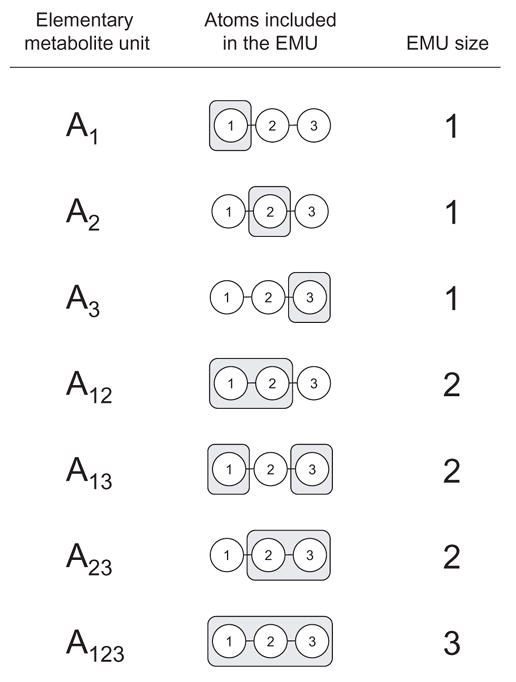
Elementary metabolite units (EMU) are distinct subsets of the compound’s atoms. There are 7 EMUs for a 3-atom metabolite A. The subscript in the first column and the shaded areas in the second column denote the atoms that are included in the EMU. The EMU size is the number of atoms included in the EMU.

In this paper, we will illustrate that the EMU framework can be used for the simulation of isotopic labeling within a reaction network using the minimum number of variables, all of which are expressed in terms of EMUs. In most cases, only a very small fraction of all possible EMUs is required to simulate the isotopic labeling. This approach is fundamentally different from the isotopomer and cumomer methods, where the simulation model always uses the complete set of all possible isotopomer/cumomers. In the next sections, we will first illustrate the EMU approach for simulating MS measurements, and in section 2.8 we will show how NMR measurements can be simulated using EMUs.

2.2 EMU reactions

First, we need to introduce the concept of an EMU reaction. Figure 2 shows three types of biochemical reactions that we distinguish: a condensation reaction, a cleavage reaction, and a unimolecular reaction. For each reaction type in Figure 2 we would like to determine the minimum amount of information that is needed to determine the mass isotopomer distribution (MID) of product C, i.e. EMU C₁₂₃. For the condensation reaction, MID of C₁₂₃ is fully determined by MIDs of EMUs A₁₂ and B₁. For example, the M+0 abundance of C₁₂₃ is equal to the product of M+0 abundances of A₁₂ and B₁, i.e. C_123,M+0=A_12,M+0·B_1,M+0. The full MID of C₁₂₃ is obtained from the convolution (or Cauchy product, denoted by ‘×’) of MIDs of A₁₂ and B₁, i.e. C₁₂₃=A₁₂×B₁ (Figure 2). For the cleavage and unimolecular reactions, the MID of C₁₂₃ is equal to the MID of A₁₂₃. Note that for the cleavage reaction atoms of A that are not transferred to C₁₂₃ are not considered in the EMU reaction, i.e. their labeling doesn’t affect the labeling state of C. Note also that EMU reactions are always size balanced, i.e. the EMU product is formed either from EMUs of the same size, or by condensation of smaller EMUs such that the total size of substrate EMUs equals the size of the EMU product. Thus, there can only be two types of EMU reactions: condensation and unimolecular EMU reactions. Table 1 shows the EMU reactions corresponding to the biochemical reactions in Figure 2.

Figure 2.

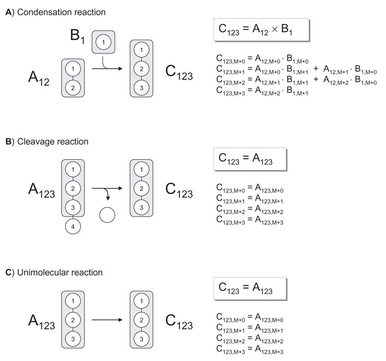
Three types of biochemical reactions with the corresponding EMU reactions. Shaded areas indicate atoms included in the EMUs. The mass isotopomer distribution (MID) of product C is fully determined by MIDs of substrate EMUs. For the condensation reaction, MID of C₁₂₃ is obtained from the convolution (or Cauchy product, denoted by ‘×’) of MIDs of A₁₂ and B₁. For the cleavage reaction and unimolecular reaction MID of C₁₂₃ equals MID of A₁₂₃.

Table 1.

EMU reactions corresponding to the reactions shown in Figure 2. Note that EMU reactions are always EMU size balanced, i.e. the size of the EMU product always equals the total size of substrate EMUs.

Reaction type	Biochemical reaction	EMU reaction	EMU size balance
Condensation	A + B → C	A12 + B1 → C123	2 + 1 = 3
Cleavage	A → B + C	A123 → C123	3 = 3
Unimolecular	A → C	A123 → C123	3 = 3

2.3 Decomposing metabolic networks into EMU reactions

We will now describe an algorithm that systematically decomposes any biochemical reaction network into EMU reactions using the knowledge of atomic transitions occurring in the network reactions. These EMU reactions will then form the basis for generating model equations for isotopic simulations (next section). Consider the example network shown in Figure 3 that will be used to illustrate the theory behind EMU decomposition. In this network, metabolite A is the sole substrate and metabolites E and F are two network products. The intermediary metabolites B, C and D are assumed to be at metabolic and isotopic steady state. The stoichiometry and atom transitions for the reactions are given in Table 2. The structural input that is required for EMU decomposition is threefold:

Figure 3.

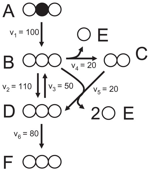
Simple metabolic network used to illustrate the decomposition of a metabolic network into EMU reactions. Atom transitions for the reactions in this model are given in Table 2. The assumed steady-state fluxes have arbitrary units and the network substrate A is labeled on the second atom.

Table 2.

Stoichiometry and atom transitions for the reactions in the example metabolic network.

Reaction number	Reaction stoichiometry	Atom transformations*
1	A → B	abc → abc
2	B ↔ D	abc ↔ abc
3	B → C + E	abc → bc + a
4	B + C → D + E + E	abc + de → bcd + a + e
5	D → F	abc → abc

^*For each metabolite atoms are identified using lower case letters to represent successive atoms of that metabolite.

1. The assumed reaction network stoichiometry

2. Atom transitions for all reactions in the network

3. List of metabolites/metabolite fragments that need to be simulated

In this example, we would like to set up the simplest possible model to simulate the MID of metabolite F, i.e. EMU F₁₂₃. The following algorithm systematically identifies all EMU reactions that are needed for this simulation model. First, we identify in the network model all EMU reactions that form EMU F₁₂₃. In this case, F₁₂₃ is formed only in reaction 6 from EMU D₁₂₃. We record this EMU reaction and the newly identified EMU(s) and repeat this process for all new EMUs, starting with the largest EMU size, i.e. D₁₂₃. Here, D₁₂₃ is formed in two reactions, i.e. in reaction 2 from B₁₂₃, and in reaction 5 from B₂₃+C₁. Next, B₁₂₃ is formed in reactions 1 and 3 from A₁₂₃ and D₁₂₃, respectively. Note that A₁₂₃ is a network substrate, i.e. it is not produced by any reaction in the network, and D₁₂₃ was already considered in the previous step. Thus, we have identified all EMU reactions of size 3 that need to be considered. Next, we proceed with EMUs of size 2 that were previously identified; here, B₂₃ is formed in reaction 1 and 3 from A₂₃, and D₂₃, respectively, etc. We complete this process for all new EMUs of size 2 and 1, until the EMUs have been traced back to EMUs of network substrates or EMUs that were already accounted for. Table 3 shows the complete EMU decomposition for this system. In this case, 18 EMU reactions were identified connecting 14 EMUs. Of these 14 EMUs, 10 EMUs correspond to intermediary metabolites whose labeling is unknown, and 4 EMUs are fully defined by the choice of substrate labeling of metabolite A. It should be clear that the described decomposition algorithm is exhaustive, unsupervised, and always identifies the minimal set of EMU reactions that need to be considered in the simulation model. Furthermore, this algorithm is easily implemented and is computationally efficient, i.e. the decomposition completes within seconds even for the largest network model that we have considered. The main advantage of the EMU decomposition is that metabolites are never broken into smaller pieces than is strictly required to describe the labeling state of the selected metabolites. In contrast, the isotopomer and cumomer frameworks always use all 2^N isotopomers per metabolite to simulate the system. In this example, the complete set of 36 isotopomers describe the system, with 28 unknown isotopomers and 8 substrate isotopomers. Thus, in this example the number of system variables was reduced by more than 50% using the EMU framework.

Table 3.

Complete list of EMU reactions generated for metabolite F with the described decomposition algorithm. Subscripts denote atoms that are included in the respective EMUs. Note that EMU reactions are always size balanced.

Reaction No.	EMU reaction	EMU reaction size balance
6	D123 → F123	3 = 3
2	B123 → D123	3 = 3
5	B23 + C1 → D123	2 + 1 = 3
1	A123 → B123	3 = 3
3	D123 → B123	3 = 3
1	A23 → B23	2 = 2
3	D23 → B23	2 = 2
2	B23 → D23	2 = 2
5	B3 + C1 → D23	1 + 1 = 2
4	B2 → C1	1 = 1
1	A2 → B2	1 = 1
3	D2 → B2	1 = 1
2	B2 → D2	1 = 1
5	B3 → D2	1 = 1
1	A3 → B3	1 = 1
3	D3 → B3	1 = 1
2	B3 → D3	1 = 1
5	C1 → D3	1 = 1

2.4 Setting up EMU balances and simulating labeling distribution

The EMU reactions obtained from network decomposition form the new basis for generating system equations. EMU reaction networks are much less connected than isotopomer systems, and we can group EMU reactions into decoupled reaction networks based on: (i) the EMU size, and (ii) network connectivity (see section 3.4 for an example). For the example network we obtain three decoupled reaction networks of EMU size 1, 2, and 3, respectively (Figure 4). Similar to metabolite and isotopomer balancing, we can set up balances around all EMUs. In general, EMU balances can be written as a set of equations that are linear in the unknown EMU variables:

Figure 4.

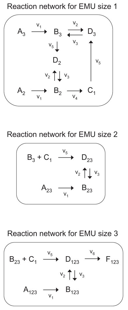
Decoupled EMU reaction networks generated for the simulation of metabolite F. Note that the EMU reaction networks contain only these EMUs that are strictly required to simulate F.

$${\text{A}}_{1,\text{k}}(\text{v})·{\text{X}}_{1,\text{k}}={\text{B}}_{1,\text{k}}(\text{v})·{\text{Y}}_{1,\text{k}}({{\text{y}}_1}^{\text{in}})$$ (1a)

$${\text{A}}_{2,\text{k}}(\text{v})·{\text{X}}_{2,\text{k}}={\text{B}}_{2,\text{k}}(\text{v})·{\text{Y}}_{2,\text{k}}({{\text{y}}_2}^{\text{in}},{\text{X}}_1)$$ (1b)

...

$${\text{A}}_{\text{n},\text{k}}(\text{v})·{\text{X}}_{\text{n},\text{k}}={\text{B}}_{\text{n},\text{k}}(\text{v})·{\text{Y}}_{\text{n},\text{k}}({{\text{y}}_{\text{n}}}^{\text{in}},{\text{X}}_{\text{n}-1},\dots ,{\text{X}}_1)$$ (1c)

Matrices X_i,k and Y_i,k represent to the unknown (balanced), and known EMU variables, respectively, and y_iⁱⁿ are EMUs of network substrates. The first subscript denotes the EMU size and the second the subnetwork number, i.e. in case there are multiple decoupled EMU networks of the same EMU size. For brevity will omit the second subscript if there is only one subnetwork of a certain EMU size. Each row in matrices Y_i,k and X_i,k contains the MID for the corresponding EMU. The EMU balances written in matrix form corresponding to the EMU networks in Figure 4 are shown below.

$$\left[\begin{array}{ccccc}-{\text{v}}_4& {\text{v}}_4& 0& 0& 0\\ 0& -{\text{v}}_1-{\text{v}}_3& {\text{v}}_3& 0& 0\\ 0& {\text{v}}_2& -{\text{v}}_2-{\text{v}}_5& {\text{v}}_5& 0\\ 0& 0& 0& -{\text{v}}_1-{\text{v}}_3& {\text{v}}_3\\ {\text{v}}_5& 0& 0& {\text{v}}_2& -{\text{v}}_2-{\text{v}}_5\end{array}\right]\hspace{0.17em}·\hspace{0.17em}\left[\begin{array}{c}{\text{C}}_1\\ {\text{B}}_2\\ {\text{D}}_2\\ {\text{B}}_3\\ {\text{D}}_3\end{array}\right]\hspace{0.17em}=\hspace{0.17em}\left[\begin{array}{cc}0& 0\\ -{\text{v}}_1& 0\\ 0& 0\\ 0& -{\text{v}}_1\\ 0& 0\end{array}\right]\hspace{0.17em}·\hspace{0.17em}\left[\begin{array}{c}{\text{A}}_2\\ {\text{A}}_3\end{array}\right]$$ (2a)

$$\left[\begin{array}{cc}-{\text{v}}_5-{\text{v}}_2& {\text{v}}_2\\ {\text{v}}_3& -{\text{v}}_1-{\text{v}}_3\end{array}\right]\hspace{0.17em}·\hspace{0.17em}\left[\begin{array}{c}{\text{D}}_{23}\\ {\text{B}}_{23}\end{array}\right]=\left[\begin{array}{cc}-{\text{v}}_5& 0\\ 0& -{\text{v}}_1\end{array}\right]\hspace{0.17em}·\hspace{0.17em}\left[\begin{array}{c}{\text{B}}_3\times {\text{C}}_1\\ {\text{A}}_{23}\end{array}\right]$$ (2b)

$$\left[\begin{array}{ccc}-{\text{v}}_6& {\text{v}}_6& 0\\ 0& -{\text{v}}_5-{\text{v}}_2& {\text{v}}_2\\ 0& {\text{v}}_3& -{\text{v}}_1-{\text{v}}_3\end{array}\right]\hspace{0.17em}·\hspace{0.17em}\left[\begin{array}{c}{\text{F}}_{123}\\ {\text{D}}_{123}\\ {\text{B}}_{123}\end{array}\right]=\left[\begin{array}{cc}0& 0\\ -{\text{v}}_5& 0\\ 0& -{\text{v}}_1\end{array}\right]\hspace{0.17em}·\hspace{0.17em}\left[\begin{array}{c}{\text{B}}_{23}\times {\text{C}}_1\\ {\text{A}}_{123}\end{array}\right]$$ (2c)

The product term B₃×C₁ in Eq. 2b represents the convolution of MIDs of B₃ and C₁ (see section 2.2). Matrices X₂ and Y₂ written out in full for the example network are shown below.

$$\left[\begin{array}{c}{\text{D}}_{23}\\ {\text{B}}_{23}\end{array}\right]=\left[\begin{array}{ccc}{\text{D}}_{23,\text{M}+0}& {\text{D}}_{23,\text{M}+1}& {\text{D}}_{23,\text{M}+2}\\ {\text{B}}_{23,\text{M}+0}& {\text{B}}_{23,\text{M}+1}& {\text{B}}_{23,\text{M}+2}\end{array}\right]$$ (3)

$$\left[\begin{array}{c}{\text{B}}_3\times {\text{C}}_1\\ {\text{A}}_{23}\end{array}\right]=\left[\begin{array}{ccc}{\text{B}}_{3,\text{M}+0}·{\text{C}}_{1,\text{M}+0}& ({\text{B}}_{3,\text{M}+0}·{\text{C}}_{1,\text{M}+1}+{\text{B}}_{3,\text{M}+1}·{\text{C}}_{1,\text{M}+0})& {\text{B}}_{3,\text{M}+1}·{\text{C}}_{1,\text{M}+1}\\ {\text{A}}_{23,\text{M}+0}& {\text{A}}_{23,\text{M}+1}& {\text{A}}_{23,\text{M}+2}\end{array}\right]$$ (4)

The size of matrix A_i depends on the number of balanced EMUs, and the size of matrix B_i depends on the number of input EMUs in that EMU network. Thus, for n balanced and m input EMUs, A_i is an n × n matrix and B_i is an n × m matrix. Note that matrices A_i and B_i are always strictly linear functions of fluxes, i.e. dA_i/dv_j and dB_i/dv_j are constant for any metabolic system. To simulate the isotopic labeling distribution for the selected metabolites, EMU balances are solved sequentially starting with the smallest EMU size network. Since the matrix Y₁ is known, i.e. it is fully determined by EMUs of network substrate A, we can easily calculate X₁ using standard linear algebra techniques:

$${\text{X}}_{\text{i}}={{\text{A}}_{\text{i}}}^{-1}·{\text{B}}_{\text{i}}·{\text{Y}}_{\text{i}}$$ (5)

For subsequent EMU networks, matrices Y_i may depend on previously determined EMUs of smaller size. Thus, for larger EMU sizes we must first update matrix Y_i and then calculate X_i. After all EMUs have been computed we can simply read out the simulated MIDs for the selected metabolites of interest from the rows of matrices X_i. For example, the MID of F₁₂₃ is found in the first row of matrix X₃.

2.5 Calculating first order derivatives of simulated measurements

Flux estimation algorithms and algorithms used for calculating flux confidence intervals require repeated calculation of first order derivatives, i.e. sensitivities of simulated measurements with respect to fluxes (Antoniewicz et al., 2006). Here, we present analytical expressions for the calculation of these sensitivities from EMU balances. In general, EMU balances are expressed in the following matrix form:

$${\text{A}}_{\text{i}}·{\text{X}}_{\text{i}}={\text{B}}_{\text{i}}·{\text{Y}}_{\text{i}}$$ (6)

where matrices A_i and B_i are strictly linear functions of fluxes and matrices X_i and Y_i are nonlinear functions of fluxes. Implicit differentiation of Eq. 6 yields:

$$\frac{{\text{dA}}_{\text{i}}}{\text{dv}}·{\text{X}}_{\text{i}}+{\text{A}}_{\text{i}}·\frac{{\text{dX}}_{\text{i}}}{\text{dv}}=\frac{{\text{dB}}_{\text{i}}}{\text{dv}}·{\text{Y}}_{\text{i}}+{\text{B}}_{\text{i}}·\frac{{\text{dY}}_{\text{i}}}{\text{dv}}$$ (7)

Note that matrices dA_i/dv_j and dB_i/dv_j are constant for a given metabolic system. After rearrangement of Eq. 7 we obtain the following general expression for dX_i/dv:

$$\frac{{\text{dX}}_{\text{i}}}{\text{dv}}={{\text{A}}_{\text{i}}}^{-1}·\left(\frac{{\text{dB}}_{\text{i}}}{\text{dv}}·{\text{Y}}_{\text{i}}+{\text{B}}_{\text{i}}·\frac{{\text{dY}}_{\text{i}}}{\text{dv}}-\frac{{\text{dA}}_{\text{i}}}{\text{dv}}·{\text{X}}_{\text{i}}\right)$$ (8)

The above expression may be simplified for the smallest EMU size network, where all terms in matrix Y are given by network substrates and thus are constant, i.e. dY/dv=0. For EMU networks of larger EMU size, matrices Y_i may depend on previously determined EMUs of smaller size. In the example network Y₂ was given by:

$${\text{Y}}_2=\left[\begin{array}{c}{\text{B}}_3\times {\text{C}}_1\\ {\text{A}}_{23}\end{array}\right]$$ (9)

Where, B₃ and C₁ are EMUs of size 1 that are calculated from EMU size 1 balances. Application of the product rule yields the following expression for the first order derivative of the convolution of B₃ and C₁ (i.e. first row of Y₂):

$$\frac{\text{d}}{\text{dv}}\left({\text{B}}_3\times {\text{C}}_1\right)=\frac{{\text{dB}}_{\text{3}}}{\text{dv}}\times {\text{C}}_1+{\text{B}}_3\times \frac{{\text{dC}}_{\text{1}}}{\text{dv}}$$ (10)

where matrices dC₁/dv and dB₃/dv are obtained from the previously determined matrix dX₁/dv. Note that the second row of Y₂ contains A₂₃ which is a network substrate EMU, i.e. it is considered constant (dA₂₃/dv=0). Thus, we obtain the following expression for dY₂/dv:

$$\frac{{\text{dY}}_{\text{2}}}{\text{dv}}=\left[\begin{array}{c}\frac{{\text{dB}}_{\text{3}}}{\text{dv}}\times {\text{C}}_1+{\text{B}}_3\times \frac{{\text{dC}}_{\text{1}}}{\text{dv}}\\ 0\end{array}\right]$$ (11)

where (dB₃/dv)×C₁ denotes the 2D-convolution of matrix (dB₃/dv) and vector C₁. Thus, first order derivatives for any EMU size can be obtained sequentially from the EMU balances. Figure 5 summarizes the general procedure for simulating labeling distributions and calculating first order derivatives of simulated measurements with respect to fluxes using the EMU framework.

Figure 5.

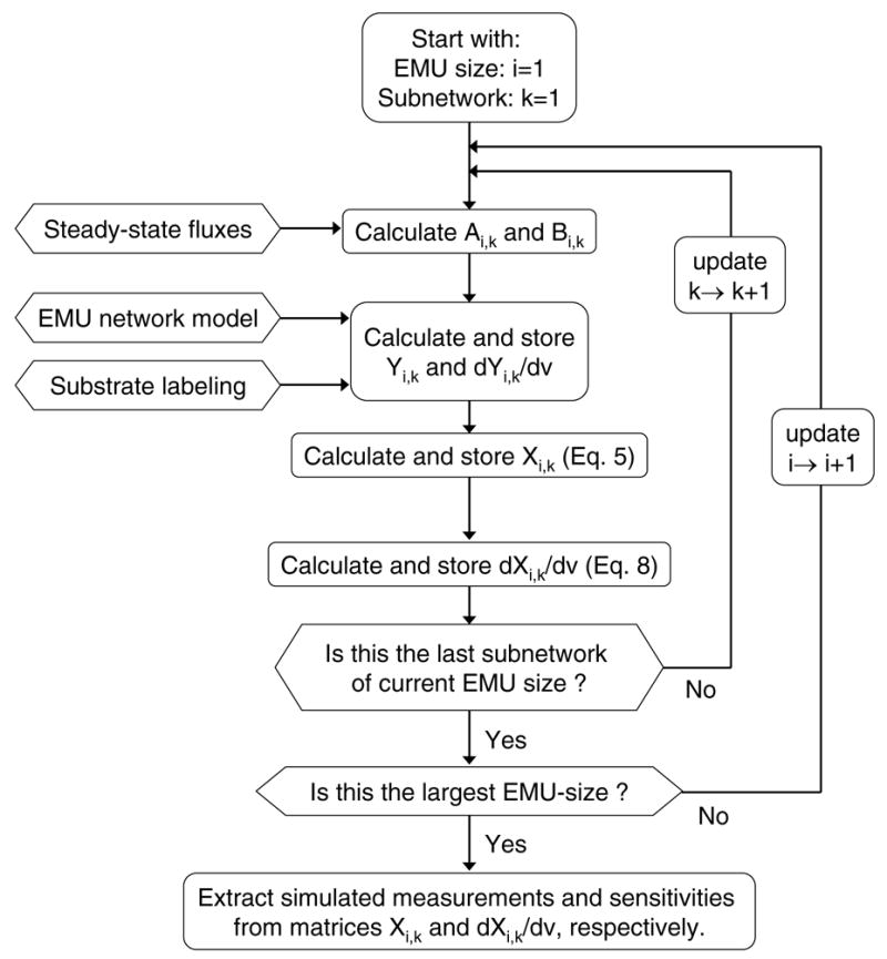
A schematic of the algorithm for simulating labeling distributions and calculating sensitivities from EMU balances. EMU balances are solved sequentially starting with the smallest EMU-size networks up to the largest EMU-size network. The simulated measurements and sensitivities are extracted from matrices X and dX/dv, respectively.

2.6 Global stability and computation time of EMU simulations

For non-zero fluxes matrices A_i are compartmental matrices, and from compartmental matrix theory we know that therefore matrices A_i are always invertible (Anderson, 1983). In other words, the EMU approach will always compute a unique and stable solution for all EMUs. The most time-consuming operation in solving EMU balances and calculating sensitivities is the inversion of matrices A_i, or rather matrix factorization of A_i. In general, the computational time for LU decomposition increases with the size of the matrix, i.e. the number of EMU nodes for each subnetwork. We found empirically that for sparsely connected EMU networks, such as the ones shown in Figure 4, the computation time increased linearly with the number of EMUs, i.e. O(n). For more highly connected networks, for example, the EMU networks corresponding to central carbon metabolism of E. coli (section 3.4), the computational time increased to the third power of the number of EMUs, i.e. O(n³). Thus, it will often be worthwhile to reduce the number of EMUs by eliminating EMU nodes that have a single influx. This will be illustrated in detail in section 3.3.

2.7 Identifying equivalent EMUs of metabolites

There is a number of considerations regarding the chemical structure of metabolites that need to be taken into account for EMU simulation models. Here, we will discuss in detail how to account for chiral, prochiral and rotationally symmetric metabolites, and how biochemically equivalent hydrogen, oxygen and other atoms should be modeled within the EMU framework. These considerations are equally important for the construction of isotopomer models, however, until now they have not received proper attention.

2.7.1 Chiral and prochiral metabolites

Tetrahedral carbon atoms with four different ligands are called chiral, whereas the term prochiral applies to carbon atoms that hold two stereoheterotopic groups (Moss, 1996). Many biological metabolites contain one or more chiral and/or prochiral carbon atoms. It is well known that biochemical reactions are highly stereospecific, i.e. enzymes differentiate between prochiral atoms and prochiral atom groups. Therefore, it is important to keep track of individual prochiral atoms in a network model and assign stereospecific atom transitions to all biochemical reactions. Consider for example the enzymatic reaction catalyzed by aconitase that converts citrate to isocitrate (Figure 6). Three of the six carbon atoms of citrate are prochiral, i.e. C2, C3 and C4. The enzyme aconitase stereospecifically transfers the pro-R hydrogen from the pro-R arm (i.e. C1-C2) of citrate to C3 of isocitrate, and produces only one of four possible stereoisomers of isocitrate, i.e. (2R,3S)-isocitrate. Note also that the prochirality of C4 is not altered by aconitase. The absolute stereochemistry for many bioreactions has been worked out in detail and can be found in biochemistry textbooks and other general literature.

Figure 6.

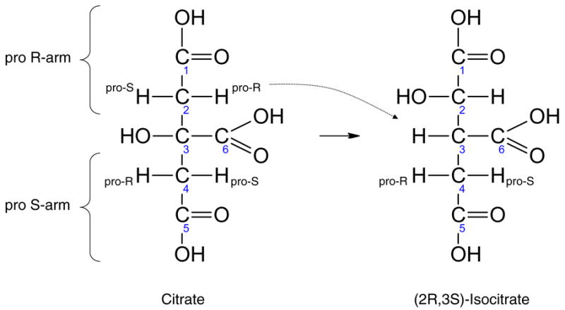
Stereospecific atom transitions for the reaction catalyzed by aconitese. Aconitase stereospecifically transfers the pro-R hydrogen from the pro-R arm of citrate to C3 of isocitrate, and produces only one of four possible stereoisomers of isocitrate, i.e. (2R,3S)-isocitrate.

2.7.2 Equivalent hydrogen and oxygen atoms

Biological molecules often contain groups of atoms that are biochemically indistinguishable. If we assume that there is no metabolic channeling, then this results in rapid equilibration of labeling at these positions. Consider for example the chemical structure of pyruvate shown in Figure 7. The three hydrogen atoms at C3 are biochemically equivalent, i.e. enzymes cannot distinguish between these atoms. Furthermore, the two oxygen atoms at C1 are biochemically equivalent due to resonance stabilization. Thus, not all of pyruvate’s EMUs are independent. For example, there are six equivalent EMUs of pyruvate that contain three carbon atoms, two of the three hydrogen atoms at C3, and one of two oxygen atom at C1. Figure 7 shows the six equivalent EMUs. We can predict the number of equivalent EMUs for any EMU as follows:

Figure 7.

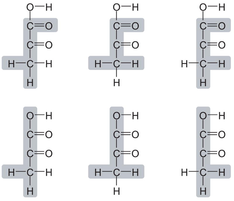
Six equivalent EMUs of pyruvate. Three hydrogen atoms of pyruvate at C3 are biochemically equivalent, and two oxygen atoms at C1 are equivalent due to resonance stabilization. As such, there are six equivalent EMUs of pyruvate containing all three carbon atoms, two of the three hydrogen atoms at C3, and one of two oxygen atom at C1. Shaded areas indicate atoms that are included in the EMUs.

$$\text{No}.\hspace{0.17em}\text{of\hspace{0.17em}equivalent\hspace{0.17em}EMUs}=\prod _{\begin{array}{l}\text{for\hspace{0.17em}each\hspace{0.17em}group\hspace{0.17em}of}\\ \text{equivalent\hspace{0.17em}atoms}\end{array}}\left(\begin{array}{c}\text{No}.\hspace{0.17em}\text{of\hspace{0.17em}equivalent\hspace{0.17em}atoms\hspace{0.17em}in\hspace{0.17em}the}\hspace{0.17em}\text{group}\\ \text{No}.\hspace{0.17em}\text{of\hspace{0.17em}these\hspace{0.17em}atoms\hspace{0.17em}in\hspace{0.17em}the\hspace{0.17em}EMU}\end{array}\right)$$ (12)

When setting up EMU balances, we need to account for the presence of equivalent EMUs. We propose the following method. First, whenever a new EMU is generated during EMU network decomposition, we identify all equivalent EMUs for that EMU. Then, for each equivalent EMU we find the EMU reaction(s) that produce that EMU, and divide the contribution from each reaction by the total number of equivalent EMUs. Note that this way we introduce only one EMU variable for each group of equivalent EMUs. For example, consider the enzymatic reaction catalyzed by malic enzyme that converts malate to pyruvate shown in Figure 8 (arbitrary numbering of atoms). The six equivalent EMUs of pyruvate from Figure 7 are produced by the following six EMU reactions:

Figure 8.

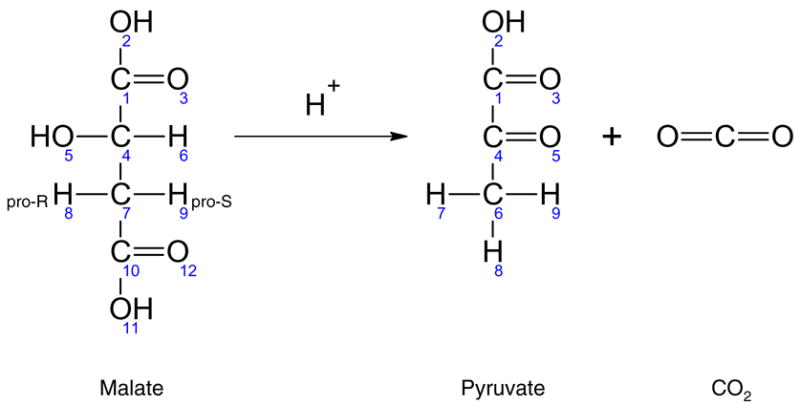
Malic enzyme converts malate to pyruvate. Note that one of the three hydrogen atoms at C_#6 of pyruvate is derived from the solvent. The two prochiral hydrogen atoms of malate at C_#7, which are biochemically distinct, become indistinguishable after malate is converted to pyruvate.

$${\text{Mal}}_{13478}+\text{H}\to {\text{Pyr}}_{134678}$$ (13a)

$${\text{Mal}}_{134789}\to {\text{Pyr}}_{134679}$$ (13b)

$${\text{Mal}}_{13479}+\text{H}\to {\text{Pyr}}_{134689}$$ (13c)

$${\text{Mal}}_{12478}+\text{H}\to {\text{Pyr}}_{124678}$$ (13d)

$${\text{Mal}}_{124789}\to {\text{Pyr}}_{124679}$$ (13e)

$${\text{Mal}}_{12479}+\text{H}\to {\text{Pyr}}_{124689}$$ (13f)

We can represent these 6 equivalent EMUs of pyruvate by a single EMU variable {Pyr₁₃₄₆₇₈}, where the brackets denote the presence of multiple equivalent EMUs. Next, we also identify that Mal₁₃₄₇₈ and Mal₁₂₄₇₈; Mal₁₃₄₇₉ and Mal₁₂₄₇₉; and Mal₁₃₄₇₈₉ and Mal₁₂₄₇₈₉ are equivalent EMUs. Taken together, we obtain the following overall EMU reaction for the production of {Pyr₁₃₄₆₇₈}:

$$\left\{{\text{Pyr}}_{134678}\right\}=\frac{1}{3}\left\{{\text{Mal}}_{13478}\right\}\times \text{H}+\frac{1}{3}\left\{{\text{Mal}}_{13479}\right\}\times \text{H}+\frac{1}{3}\left\{{\text{Mal}}_{134789}\right\}$$ (14)

Thus, {Pyr₁₃₄₆₇₈} is formed from three EMUs of malate, i.e. {Mal₁₃₄₇₈}, {Mal₁₃₄₇₉}, and {Mal₁₃₄₇₈₉}; two groups are of EMU size 5 that combine with H⁺, and one is of EMU size 6. Note also that the two prochiral hydrogen atoms of malate that are initially biochemically distinct become indistinguishable after malate is converted to pyruvate.

Rotationally symmetric metabolites

A number of metabolites of central carbon metabolism are rotationally symmetric, i.e. they are superposable on themselves by rotation. In isotopic labeling studies these molecules also cause scrambling of isotopic labeling. It is important to note that there is a clear difference between molecules with a rotation axis and molecules with a center of inversion (Moss, 1996). The two types of symmetry have different characteristics. Only molecules with a rotation axis are superposable on themselves. Figure 9 shows the structures of (2S,3R)-butane-1,2,3,4-tetraol (i.e. erythritol) which has a center of inversion, and (2R,3R)-butane-1,2,3,4-tetraol which has a rotation axis. Carbon atoms C1 and C4, and C2 and C3 of erythriol are chemically equivalent, i.e. they react identically in chemical reactions and have the same chemical properties, however, in enzymatic reactions these groups are biochemically distinct. In contrast, carbon atoms C1 and C4, and C2 and C3 of (2R,3R)-butane-1,2,3,4-tetraol are both chemically and biochemically equivalent, i.e. they are not distinguished by enzymes, and thus result in label scrambling.

Figure 9.

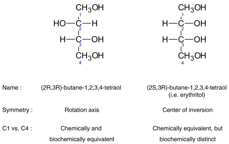
Differences between molecules with a rotation axis and center of inversion. (2S,3R)-Butane-1,2,3,4-tetraol (i.e. erythritol) has a center of inversion and is not superposable on itself. Thus, carbon atoms C1 and C4, and C2 and C3 of erythritol are biochemically distinct. (2R,3R)-Butane-1,2,3,4-tetraol, on the other hand, has a rotation axis and is superposable on itself. Hence, carbon atoms C1 and C4, and C2 and C3 are biochemically indistinguishable, resulting in scrambling of isotopic labeling.

The most important examples of rotationally symmetric molecules in central metabolism are fumarate, succinate, and D-mannitol. Figure 10 shows the structure of fumarate (with arbitrary numbering of atoms). It should be clear that fumarate has a rotation axis, i.e. after rotating 180° fumarate superposes on itself. Furthermore, the two oxygen atoms at the first carbon and the two oxygen atoms at the last carbon atom are biochemically equivalent due to resonance stabilization. These characteristics of fumarate need to be considered when we identify equivalent EMUs of fumarate. It should also be clear that the number of equivalent EMUs may increase due to rotational symmetry. EMUs of rotationally symmetric molecules may have twice as many equivalent EMUs as nonsymmetric molecules, assuming a rotational symmetry of 180 degrees. The multiplier will increase if the angle is less, e.g. in benzene where the rotational symmetry is 60 degrees the multiplier would be 6 (=360/6)

Figure 10.

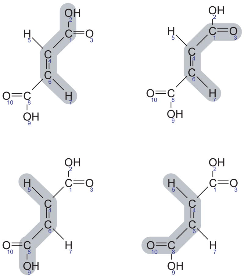
Equivalent EMUs of fumarate, a rotationally symmetric molecule. The following four EMUs are equivalent: Fum₁₂₄₆₇, Fum₁₃₄₆₇, Fum₄₅₆₈₉, and Fum_4568,10 (numbering of fumarate atoms is arbitrary). Shaded areas indicate atoms included in the EMUs.

$$\text{No}.\hspace{0.17em}\text{of\hspace{0.17em}equivalent\hspace{0.17em}EMUs}\le \text{2}\times \prod _{\begin{array}{l}\text{for\hspace{0.17em}each\hspace{0.17em}group\hspace{0.17em}of}\\ \text{equivalent\hspace{0.17em}atoms}\end{array}}\left(\begin{array}{c}\text{No}.\hspace{0.17em}\text{of}\hspace{0.17em}\text{equivalent\hspace{0.17em}atoms\hspace{0.17em}in\hspace{0.17em}the\hspace{0.17em}group}\\ \text{No}.\hspace{0.17em}\text{of\hspace{0.17em}these}\hspace{0.17em}\text{atoms\hspace{0.17em}in\hspace{0.17em}the\hspace{0.17em}EMU}\end{array}\right)$$ (15)

Figure 10 shows, for example, the four equivalent EMUs of fumarate Fum₁₂₄₆₇. Note also, for example, that fumarate EMU F₁₄₆₈ has no equivalent EMUs, because its rotational equivalent is F₁₄₆₈ itself. Hence, when we enumerate equivalent EMUs it is very important that we separate the effects of rotational symmetry, which is a global characteristic of a molecule, from the effects of equivalent hydrogen and oxygen atoms, which are local characteristics. To better illustrate this, consider hydrogen atoms #5 and #7 of fumarate in Figure 10. These atoms cannot be treated as equivalent atoms, because that would incorrectly identify Fum₁₂₄₆₅ as being equivalent to Fum₁₂₄₆₇. Taking these considerations into account, Figure 11 shows the complete algorithm for decomposing metabolic networks into EMU reaction networks.

Figure 11.

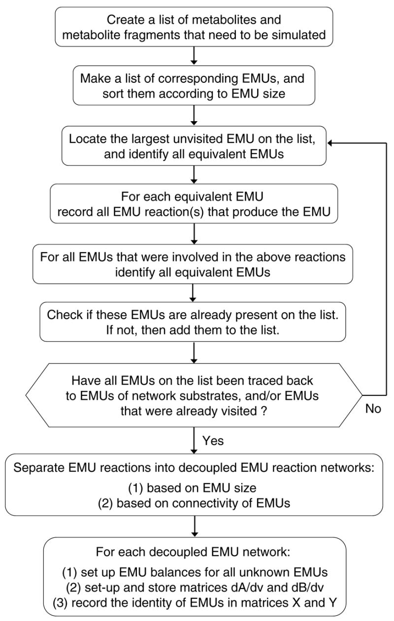
A schematic of the algorithm for the decomposition of metabolic networks into decoupled EMU networks. This algorithm systematically identifies the minimal set of EMU reactions that are needed for the simulation model. The algorithm is exhaustive, unsupervised, and computationally efficient.

2.8 Simulating NMR measurements using EMUs

Thus far, we have shown how MS measurements can be simulated using the EMU approach. We will now illustrate the method for simulating NMR measurements, in particular we will show how fractional enrichments and NMR fine spectra can be simulated.

2.8.1 Simulation of fractional enrichments

Fractional enrichments are a measure of the fractional abundance of ¹³C-atoms at specific carbon positions in a molecule. For example, Wiechert et al. (Wiechert et al., 1997) measured fractional enrichments of 25 carbon atoms of amino acids. In the EMU framework fractional enrichments are modeled by EMUs of size 1, i.e. containing a single carbon atom. Thus, to simulate fractional enrichments we can simply solve EMU balances of size 1. Network decomposition is accomplished with the same algorithm as was described before (section 2.3). In the EMU balances (Eq. 1), X_i and Y_i can now be represented by vectors that contain the fractional labeling of carbon atoms. Note that the EMU method for simulating fractional enrichments is very similar to the atom mapping matrix method that was originally proposed by Zupke and Stephanopoulos (Zupke and Stephanopoulos, 1994), and the weight-1 cumomer method as proposed by Wiechert et al. (Wiechert et al., 1999).

2.8.2 Simulation of NMR fine spectra

Data obtained from 2D [¹³C,¹H] COSY spectra, also known as NMR fine spectra, provide information on the relative amount of ¹³C-¹³C and ¹³C-¹²C carbons at specific carbon positions, where the observed carbon atom is always ¹³C-labeled and the adjacent carbon atoms are either labeled or unlabeled (Szyperski, 1995). For a secondary carbon atom, NMR fine spectra can be expressed as ratios of four isotopomer fractions, i.e. A₀₁₀, A₀₁₁, A₁₁₀, and A₁₁₁:

$$\left[\begin{array}{c}\text{singlet}\\ \text{doublet\hspace{0.17em}}3\\ \text{doublet\hspace{0.17em}}1\\ \text{doublet\hspace{0.17em}doublet}\end{array}\right]=\left[\begin{array}{c}{\text{A}}_{010}\\ {\text{A}}_{011}\\ {\text{A}}_{110}\\ {\text{A}}_{111}\end{array}\right]\hspace{0.17em}·\hspace{0.17em}{({\text{A}}_{010}+{\text{A}}_{011}+{\text{A}}_{110}+{\text{A}}_{111})}^{-1}$$ (16)

We can obtain these four isotopomer fractions from cumomer fractions A_x1x, A_x11, A_11x, and A₁₁₁, as was shown previously by van Winden et al. (van Winden et al., 2002). According to the definition by Wiechert et al. (Wiechert et al., 1999), A_x1x denotes the weight-1 cumomer fraction for which the second atom is ¹³C-labeled and the other two atoms are labeled or unlabeled, i.e. x = ‘0 or 1’. Alternatively, we have derived that the same isotopomer fractions can also be obtained from the following four EMUs: A₂, A₂₃, A₁₂, and A₁₂₃. We can easily show that cumomer fraction A_x1x is equal to the M+1 abundance of EMU A₂, i.e. the fraction of fully labeled EMU A₂; weight-2 cumomer fractions A_11x and A_x11 are equal to the M+2 abundances of EMUs A₂₃ and A₁₂, respectively (i.e. fully labeled EMUs); and weight-3 cumomer fraction A₁₁₁ is equal to the M+3 abundance of EMU A₁₂₃ (i.e. fully labeled EMUs).

$$\left[\begin{array}{c}{\text{A}}_{010}\\ {\text{A}}_{110}\\ {\text{A}}_{011}\\ {\text{A}}_{111}\end{array}\right]={\left[\begin{array}{cccc}1& 1& 1& 1\\ 0& 1& 0& 1\\ 0& 0& 1& 1\\ 0& 0& 0& 1\end{array}\right]}^{-1}·\hspace{0.17em}\left[\begin{array}{c}{\text{A}}_{\text{x}1\text{x}}\\ {\text{A}}_{\text{x}11}\\ {\text{A}}_{11\text{x}}\\ {\text{A}}_{111}\end{array}\right]={\left[\begin{array}{cccc}1& 1& 1& 1\\ 0& 1& 0& 1\\ 0& 0& 1& 1\\ 0& 0& 0& 1\end{array}\right]}^{-1}·\hspace{0.17em}\left[\begin{array}{c}{\text{A}}_2\\ {\text{A}}_{23}\\ {\text{A}}_{12}\\ {\text{A}}_{123}\end{array}\right]$$ (17)

Thus, we can simulate NMR fine spectra either by solving weight-1, 2, and 3 cumomer balances (van Winden et al., 2002), or alternatively by solving EMU balances for the EMUs A₂, A₂₃, A₁₂, and A₁₂₃. For convenience, X_i and Y_i can be represented as vectors (not matrices) that contain the fractional abundances of the fully labeled EMUs. It should be clear that the number of EMUs generated for the EMUs of size 1, 2, and 3 will always be smaller, or equal to the number of weight-1, 2, and 3 cumomers. Therefore, it is always more efficient to simulate NMR fine spectra using the EMU framework.

The EMU framework can be extended even further to capture NMR fine spectra for tertiary carbon atoms, and long-range ¹³C-¹³C couplings. In that case, the following eight EMUs need to be simulated: A₂, A₁₂, A₂₃, A₂₄, A₁₂₃, A₂₃₄, A₁₂₄, and A₁₂₃₄. After simulation of these EMUs, we can convert the calculated fractional abundances of fully labeled EMUs to isotopomer fractions using Eq. 18, and then to NMR signal intensities using Eq. 19.

$$\left[\begin{array}{c}{\text{A}}_{0100}\\ {\text{A}}_{0101}\\ {\text{A}}_{0110}\\ {\text{A}}_{0111}\\ {\text{A}}_{1100}\\ {\text{A}}_{1101}\\ {\text{A}}_{1110}\\ {\text{A}}_{1111}\end{array}\right]={\left[\begin{array}{cccccccc}1& 1& 1& 1& 1& 1& 1& 1\\ 0& 1& 0& 1& 0& 1& 0& 1\\ 0& 0& 1& 1& 0& 0& 1& 1\\ 0& 0& 0& 1& 0& 0& 0& 1\\ 0& 0& 0& 0& 1& 1& 1& 1\\ 0& 0& 0& 0& 0& 1& 0& 1\\ 0& 0& 0& 0& 0& 0& 1& 1\\ 0& 0& 0& 0& 0& 0& 0& 1\end{array}\right]}^{-1}\hspace{0.17em}·\hspace{0.17em}\left[\begin{array}{c}{\text{A}}_2\\ {\text{A}}_{24}\\ {\text{A}}_{23}\\ {\text{A}}_{234}\\ {\text{A}}_{12}\\ {\text{A}}_{124}\\ {\text{A}}_{123}\\ {\text{A}}_{1234}\end{array}\right]$$ (18)

$$\left[\begin{array}{c}\text{singlet}\\ \text{doublet\hspace{0.17em}}4\\ \text{doublet\hspace{0.17em}}3\\ \text{double\hspace{0.17em}doublet\hspace{0.17em}34}\\ \text{doublet\hspace{0.17em}1}\\ \text{double\hspace{0.17em}doublet\hspace{0.17em}14}\\ \text{double\hspace{0.17em}doublet\hspace{0.17em}13}\\ \text{quadruple\hspace{0.17em}doublet}\end{array}\right]=\left[\begin{array}{c}{\text{A}}_{0100}\\ {\text{A}}_{0101}\\ {\text{A}}_{0110}\\ {\text{A}}_{0111}\\ {\text{A}}_{1100}\\ {\text{A}}_{1101}\\ {\text{A}}_{1110}\\ {\text{A}}_{1111}\end{array}\right]\hspace{0.17em}·\hspace{0.17em}{\left({\text{A}}_{0100}+{\text{A}}_{0101}+{\text{A}}_{0110}+{\text{A}}_{0111}+{\text{A}}_{1100}+{\text{A}}_{1101}+{\text{A}}_{1110}+{\text{A}}_{1111}\right)}^{-1}$$ (19)

Note that in Eqs. 18 and 19 we have assumed that the observed carbon atom is C2.

3. PRACTICAL APPLICATIONS

3.1 Simple network model

In this example we will compare the EMU framework for simulating mass isotopomer distributions to the isotopomer and cumomer frameworks. Consider the simple network model that was introduced in section 2.3 (Figure 3). The assumed steady-state fluxes and labeling of substrate A are shown in Figure 3. The solution to the EMU balances from Eq. 2 are shown below.

Solution of EMU balances for reaction network of EMU size 1

$$\left[\begin{array}{c}{\text{C}}_1\\ {\text{B}}_2\\ {\text{D}}_2\\ {\text{B}}_3\\ {\text{D}}_3\end{array}\right]={\left[\begin{array}{ccccc}-20& 20& 0& 0& 0\\ 0& -150& 50& 0& 0\\ 0& 110& -130& 20& 0\\ 0& 0& 0& -150& 50\\ 20& 0& 0& 110& -130\end{array}\right]}^{-1}·\hspace{0.17em}\left[\begin{array}{cc}0& 0\\ -100& 0\\ 0& 0\\ 0& -100\\ 0& 0\end{array}\right]\hspace{0.17em}·\hspace{0.17em}\left[\begin{array}{cc}0& 1\\ 1& 0\end{array}\right]=\left[\begin{array}{cc}0.0667& 0.9333\\ 0.0667& 0.9333\\ 0.2000& 0.8000\\ 0.9333& 0.0667\\ 0.8000& 0.2000\end{array}\right]$$

Solution of EMU balances for reaction network of EMU size 2

$$\left[\begin{array}{c}{\text{D}}_{23}\\ {\text{B}}_{23}\end{array}\right]={\left[\begin{array}{cc}-130& 110\\ 50& -150\end{array}\right]}^{-1}\hspace{0.17em}·\hspace{0.17em}\left[\begin{array}{cc}-20& 0\\ 0& -100\end{array}\right]\hspace{0.17em}·\hspace{0.17em}\left[\begin{array}{ccc}0.0622& 0.8756& 0.0622\\ 0& 1& 0\end{array}\right]=\left[\begin{array}{ccc}0.0133& 0.9733& 0.0133\\ 0.0044& 0.9911& 0.0044\end{array}\right]$$

Solution of EMU balances for reaction network of EMU size 3

$$\begin{array}{c}\left[\begin{array}{c}{\text{F}}_{123}\\ {\text{D}}_{123}\\ {\text{B}}_{123}\end{array}\right]={\left[\begin{array}{ccc}-80& 80& 0\\ 0& -130& 110\\ 0& 50& -150\end{array}\right]}^{-1}\hspace{0.17em}·\hspace{0.17em}\left[\begin{array}{cc}0& 0\\ -20& 0\\ 0& -100\end{array}\right]\hspace{0.17em}·\hspace{0.17em}\left[\begin{array}{cccc}0.0003& 0.0702& 0.9253& 0.0041\\ 0& 1& 0& 0\end{array}\right]\\ =\left[\begin{array}{cccc}0.0001& 0.8008& 0.1983& 0.0009\\ 0.0001& 0.8008& 0.1983& 0.0009\\ 0.0000& 0.9336& 0.0661& 0.0003\end{array}\right]\end{array}$$

Thus, we find that the simulated MID of F is 0.0 mol% (M+0), 80.1 mol% (M+1), 19.8 mol% (M+2), and 0.1 mol% (M+3). These simulated abundances are identical to those obtained using the isotopomer and cumomer methods. The main difference between the methods is the number of equations that was solved to simulate the labeling of metabolite F. For the isotopomer method, 28 nonlinear isotopomer balances were solved using Newton’s iterative method. With the cumomer method, 4 linear problems of size 4, 11, 10, and 3, respectively, were solved using standard linear algebra techniques. Note that the total number of cumomers was the same as the number of isotopomers. In contrast, with the EMU model 3 linear problems of size 5, 2, and 3, respectively, were solved. Table 4 summarizes the comparison between the three modeling methods for this simple example.

Table 4.

Comparison of three modeling approaches for simulating mass isotopomer labeling of F in the example network (Figure 3). The simulated abundances were identical for all methods, i.e. the EMU, isotopomer, and cumomer methods. The EMU method required 10 variables to simulate the labeling of F, as opposed to 28 variables for the isotopomer and cumomer methods (a reduction of 64%).

		isotopomer model	cumomer model	EMU model
Simulated mass isotopomer distribution of metabolite F (molfractions)	M+0	0.0001	0.0001	0.0001
	M+1	0.8008	0.8008	0.8008
	M+2	0.1983	0.1983	0.1983
	M+3	0.0009	0.0009	0.0009
Type of model equations		nonlinear	linear	linear
Number of variables in each subproblem		28	4, 11, 10, 3	5, 2, 3
Total number of variables		28	28	10

3.2 Tricarboxylic acid cycle

The second example that we consider is the simplified model of the tricarboxylic acid (TCA) cycle shown in Figure 12. The stoichiometry and atom transitions for the eight reactions are given in Table 5. In this network, acetyl coenzyme A and aspartate are the two substrates, and glutamate and carbon dioxide are the products. Here, we simulated the steady-state labeling distribution of glutamate assuming a mixture of 25% [2-¹³C]AcCoA and 25% [1,2-¹³C]AcCoA as the tracer input. The assumed flux distribution is shown in Figure 12. In this example, we only considered the labeling of carbon atoms and for simplicity ignored natural isotope enrichments. The algorithm described in section 2.3 decomposed the TCA cycle network into 4 decoupled EMU reaction networks that are shown in Figure 13. The total number of balanced EMUs was 24, i.e. 8 EMUs in the first network (EMU size 1), 5 EMUs in the second (EMU size 2), 8 EMUs in the third (EMU size 3), and 3 EMUs in the fourth network (EMU size 5). The EMU balances for the four decoupled networks are shown below.

Figure 12.

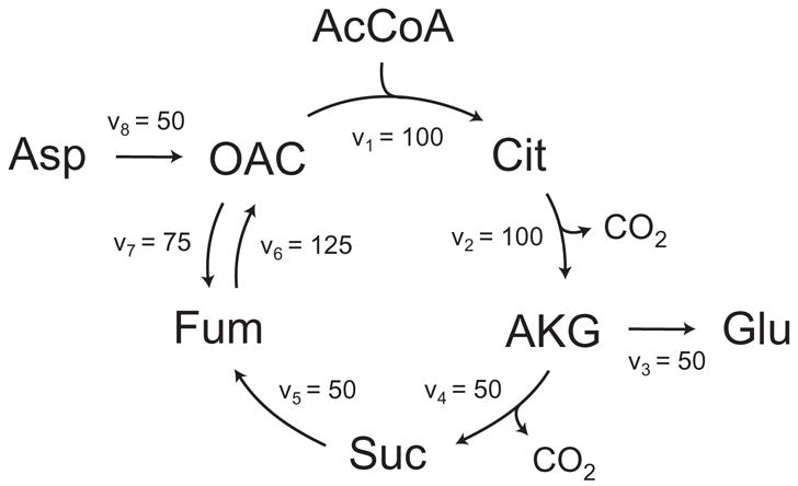
Simplified model of the tricarboxylic acid cycle. Abbreviations of metabolites: OAC, oxaloacetate; Asp, aspartate; AcCoA, acetyl coenzyme A; Cit, citrate; AKG, α-ketoglutarate; Glu, glutamate; Suc, succinate. The assumed fluxes have arbitrary units.

Table 5.

Stoichiometry and atom transitions for reactions of the TCA cycle. This network model was used to simulate the steady-state mass isotopomer distribution of glutamate.

Reaction number	Reaction stoichiometry	Carbon atom transformations*
1	OAC + AcCoA → Cit	abcd + ef → dcbfea
2	Cit → AKG + CO2	abcdef → abcde + f
3	AKG → Glu	abcde → abcde
4	AKG → Suc + CO2	abcde → bcde + a
5	Suc → Fum	½ abcd + ½ dcba → ½ abcd + ½ dcba
6	Fum → OAC	½ abcd + ½ dcba → abcd
7	OAC → Fum	abcd → ½ abcd + ½ dcba
8	Asp → OAC	abcd → abcd

^*For each compound atoms are identified using lower case letters to represent successive atoms of each compound. Abbreviations of metabolites: OAC, oxaloacetate; Asp, aspartate; AcCoA, acetyl coenzyme A; Cit, citrate; AKG, α-ketoglutarate; Glu, glutamate; Suc, succinate.

Figure 13.

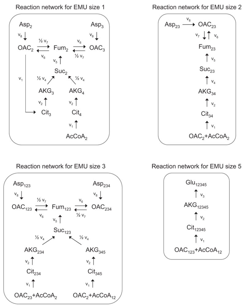
EMU reaction networks generated for glutamate from EMU network decomposition of the TCA cycle. The complete molecule of glutamate corresponds to EMU Glu₁₂₃₄₅. Subscripts denote carbon atoms that are included in the EMUs. Abbreviations of metabolites are same as in Figure 12.

$$\left[\begin{array}{cccccccc}-{\text{v}}_6-{\text{v}}_8& {\text{v}}_6& .& .& .& .& .& .\\ \frac{1}{2}{\text{v}}_7& -{\text{v}}_5-{\text{v}}_7& \frac{1}{2}{\text{v}}_7& {\text{v}}_5& .& .& .& .\\ .& {\text{v}}_6& -{\text{v}}_6-{\text{v}}_8& .& .& .& .& .\\ .& .& .& -{\text{v}}_4& \frac{1}{2}{\text{v}}_4& \frac{1}{2}{\text{v}}_4& .& .\\ .& .& .& .& -{\text{v}}_2& .& {\text{v}}_2& .\\ .& .& .& .& .& -{\text{v}}_2& .& {\text{v}}_2\\ {\text{v}}_1& .& .& .& .& .& -{\text{v}}_1& .\\ .& .& .& .& .& .& .& -{\text{v}}_1\end{array}\right]\hspace{0.17em}·\hspace{0.17em}\left[\begin{array}{c}{\text{OAC}}_2\\ {\text{Fum}}_2\\ {\text{OAC}}_3\\ {\text{Suc}}_2\\ {\text{AKG}}_3\\ {\text{AKG}}_4\\ {\text{Cit}}_3\\ {\text{Cit}}_4\end{array}\right]=\left[\begin{array}{ccc}-{\text{v}}_8& .& .\\ .& .& .\\ .& -{\text{v}}_8& .\\ .& .& .\\ .& .& .\\ .& .& .\\ .& .& .\\ .& .& -{\text{v}}_1\end{array}\right]\hspace{0.17em}·\hspace{0.17em}\left[\begin{array}{c}{\text{Asp}}_2\\ {\text{Asp}}_3\\ {\text{AcCoA}}_2\end{array}\right]$$

$$\left[\begin{array}{ccccc}-{\text{v}}_8-{\text{v}}_6& {\text{v}}_6& .& .& .\\ {\text{v}}_7& -{\text{v}}_7-{\text{v}}_5& {\text{v}}_5& .& .\\ .& .& -{\text{v}}_4& {\text{v}}_4& .\\ .& .& .& -{\text{v}}_2& {\text{v}}_2\\ .& .& .& .& -{\text{v}}_1\end{array}\right]\hspace{0.17em}·\hspace{0.17em}\left[\begin{array}{c}{\text{OAC}}_{23}\\ {\text{Fum}}_{23}\\ {\text{Suc}}_{23}\\ {\text{AKG}}_{34}\\ {\text{Cit}}_{34}\end{array}\right]=\left[\begin{array}{cc}-{\text{v}}_8& .\\ .& .\\ .& .\\ .& .\\ .& -{\text{v}}_1\end{array}\right]\hspace{0.17em}·\hspace{0.17em}\left[\begin{array}{c}{\text{Asp}}_{23}\\ {\text{OAC}}_2\times {\text{AcCoA}}_2\end{array}\right]$$

$$\begin{array}{l}\left[\begin{array}{cccccccc}-{\text{v}}_6-{\text{v}}_8& {\text{v}}_6& .& .& .& .& .& .\\ \frac{1}{2}{\text{v}}_7& -{\text{v}}_5-{\text{v}}_7& \frac{1}{2}{\text{v}}_7& {\text{v}}_5& .& .& .& .\\ .& {\text{v}}_6& -{\text{v}}_6-{\text{v}}_8& .& .& .& .& .\\ .& .& .& -{\text{v}}_4& \frac{1}{2}{\text{v}}_4& \frac{1}{2}{\text{v}}_4& .& .\\ .& .& .& .& -{\text{v}}_2& .& {\text{v}}_2& .\\ .& .& .& .& .& -{\text{v}}_2& .& {\text{v}}_2\\ .& .& .& .& .& .& -{\text{v}}_1& .\\ .& .& .& .& .& .& .& -{\text{v}}_1\end{array}\right]\hspace{0.17em}·\hspace{0.17em}\left[\begin{array}{c}{\text{OAC}}_{123}\\ {\text{Fum}}_{123}\\ {\text{OAC}}_{234}\\ {\text{Suc}}_{123}\\ {\text{AKG}}_{234}\\ {\text{AKG}}_{345}\\ {\text{Cit}}_{234}\\ {\text{Cit}}_{345}\end{array}\right]\\ =\left[\begin{array}{cccc}-{\text{v}}_8& .& .& .\\ .& .& .& .\\ .& -{\text{v}}_8& .& .\\ .& .& .& .\\ .& .& .& .\\ .& .& .& .\\ .& .& -{\text{v}}_1& .\\ .& .& .& -{\text{v}}_1\end{array}\right]\hspace{0.17em}·\hspace{0.17em}\left[\begin{array}{c}{\text{Asp}}_{123}\\ {\text{Asp}}_{234}\\ {\text{OAC}}_{23}\times {\text{AcCoA}}_2\\ {\text{OAC}}_2\times {\text{AcCoA}}_{12}\end{array}\right]\\ \left[\begin{array}{ccc}-{\text{v}}_3& {\text{v}}_3& .\\ .& -{\text{v}}_2& {\text{v}}_2\\ .& .& -{\text{v}}_1\end{array}\right]\hspace{0.17em}·\hspace{0.17em}\left[\begin{array}{c}{\text{Glu}}_{12345}\\ {\text{AKG}}_{12345}\\ {\text{Cit}}_{12345}\end{array}\right]\\ =\left[\begin{array}{c}.\\ .\\ -{\text{v}}_1\end{array}\right]\hspace{0.17em}·\hspace{0.17em}\left[{\text{OAC}}_{123}\times {\text{AcCoA}}_{12}\right]\end{array}$$

Rotational symmetric molecules fumarate and succinate were modeled as described in section 2.7, and the following groups of EMUs were identified as equivalent: Fum₂ and Fum₃; Suc₂ and Suc₃; Fum₁₂₃ and Fum₂₃₄; Suc₁₂₃ and Suc₂₃₄. Note that the EMU model only contains EMUs of size 5 and smaller, even though citrate contains 6 carbon atoms. This is direct consequence of the EMU decomposition, and clearly illustrates the advantage of the EMU framework. The decomposition will never generate EMUs of larger size than the simulated metabolites, i.e. in this case 5 (= size of Glu₁₂₃₄₅). In contrast, the isotopomer and cumomer methods used 2⁶=64 variables for citrate. The 24 EMUs constituted a significant reduction from the complete set of 176 isotopomers/cumomers that were required to describe this system (a reduction of 86%). The cumomer model consisted of seven subproblems of size 6, 28, 53, 52, 28, 8, and 1, respectively. As expected, all three modeling methods, i.e. EMU, isotopomer, and cumomer, simulated identical mass isotopomer abundances for glutamate: 34.64 mol% (M+0), 26.95 mol% (M+1), 27.08 mol% (M+2), 8.07 mol% (M+3), 2.86 mol% (M+4), and 0.39 mol% (M+5).

3.3 Reducing EMU balances

In section 2.6 we noted that the computational effort for solving EMU balances depends on the number of EMU nodes. It is often possible to reduce the number of EMU variables in the EMU networks by eliminating EMU nodes with a single influx. Note that no information is lost in this process. We applied this strategy to simplify the EMU networks for the TCA cycle example. The reduced EMU networks are shown in Figure 14. In this case, the number of EMUs was reduced from 24 to 9 EMUs, i.e. 95% reduction compared to the complete set of 176 isotopomers. The corresponding EMU balances are shown below.

Figure 14.

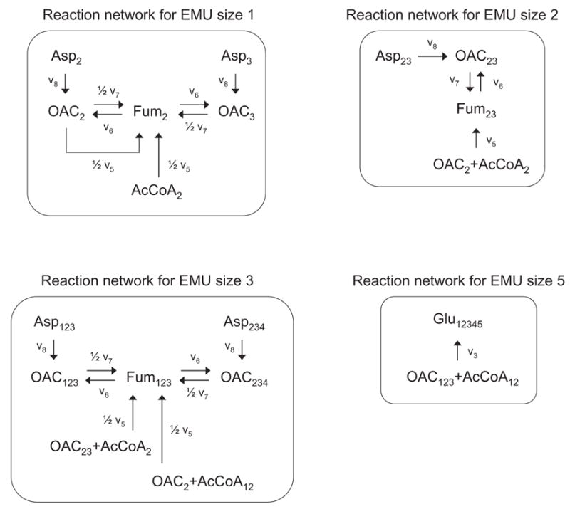
Simplified EMU reaction networks for glutamate. The EMU networks from Figure 13 were reduced by lumping linear EMU nodes having only one influx. Abbreviations of metabolites are same as in Figure 12.

$$\left[\begin{array}{ccc}-{\text{v}}_8-{\text{v}}_6& {\text{v}}_6& 0\\ \frac{1}{2}{\text{v}}_7+\frac{1}{2}{\text{v}}_5& -{\text{v}}_5-{\text{v}}_7& \frac{1}{2}{\text{v}}_7\\ 0& {\text{v}}_6& -{\text{v}}_8-{\text{v}}_6\end{array}\right]\hspace{0.17em}·\hspace{0.17em}\left[\begin{array}{c}{\text{OAC}}_2\\ {\text{Fum}}_2\\ {\text{OAC}}_3\end{array}\right]=\left[\begin{array}{ccc}-{\text{v}}_8& 0& 0\\ 0& 0& -\frac{1}{2}{\text{v}}_5\\ 0& -{\text{v}}_8& 0\end{array}\right]\hspace{0.17em}·\hspace{0.17em}\left[\begin{array}{c}{\text{Asp}}_2\\ {\text{Asp}}_3\\ {\text{AcCoA}}_2\end{array}\right]$$

$$\left[\begin{array}{cc}-{\text{v}}_8-{\text{v}}_6& {\text{v}}_6\\ {\text{v}}_7& -{\text{v}}_5-{\text{v}}_7\end{array}\right]\hspace{0.17em}·\hspace{0.17em}\left[\begin{array}{c}{\text{OAC}}_{23}\\ {\text{Fum}}_{23}\end{array}\right]=\left[\begin{array}{cc}-{\text{v}}_8& 0\\ 0& -{\text{v}}_5\end{array}\right]\hspace{0.17em}·\hspace{0.17em}\left[\begin{array}{c}{\text{Asp}}_{23}\\ {\text{OAC}}_2\times {\text{AcCoA}}_2\end{array}\right]$$

$$\left[\begin{array}{ccc}-{\text{v}}_8-{\text{v}}_6& {\text{v}}_6& 0\\ \frac{1}{2}{\text{v}}_7& -{\text{v}}_5-{\text{v}}_7& \frac{1}{2}{\text{v}}_7\\ 0& {\text{v}}_6& -{\text{v}}_8-{\text{v}}_6\end{array}\right]\hspace{0.17em}·\hspace{0.17em}\left[\begin{array}{c}{\text{OAC}}_{123}\\ {\text{Fum}}_{123}\\ {\text{OAC}}_{234}\end{array}\right]=\left[\begin{array}{cccc}-{\text{v}}_8& 0& 0& 0\\ 0& 0& -\frac{1}{2}{\text{v}}_5& -\frac{1}{2}{\text{v}}_5\\ 0& -{\text{v}}_8& 0& 0\end{array}\right]\hspace{0.17em}·\hspace{0.17em}\left[\begin{array}{c}{\text{Asp}}_{123}\\ {\text{Asp}}_{234}\\ {\text{OAC}}_{23}\times {\text{AcCoA}}_2\\ {\text{OAC}}_3\times {\text{AcCoA}}_{12}\end{array}\right]$$

$${\text{Glu}}_{12345}={\text{OAC}}_{123}\times {\text{AcCoA}}_{12}$$

Note that with the reduced EMU model we can simulate the labeling of glutamate in this system for any steady-state fluxes and any substrate labeling by solving four very simple linear problems of size 3, 2, 3, and 1, respectively. The solutions to the EMU balances for the assumed steady-state fluxes and labeling of acetyl-CoA are shown below. As expected, the simulated MID of glutamate was identical to that obtained with the full EMU model and the isotopomer and cumomer models. Table 6 summarizes the comparison of modeling methods for the TCA cycle example.

Table 6.

Comparison of modeling approaches for the simulation of isotopomer labeling of glutamate in the TCA cycle model (Figure 12). Glutamate labeling was simulated using the EMU, isotopomer, and cumomer methods. The assumed fluxes are shown in Figure 12 and the assumed labeling of AcCoA was 25% [2-¹³C]AcCoA and 25% [1,2-¹³C]AcCoA. Simulated abundances were identical for all three methods. The reduced EMU model consisted of only 9 EMU variables, as opposed to 176 variables for the isotopomer and cumomer models (a reduction of 95%).

		isotopomer model	cumomer model	EMU full model	EMU reduced model
Simulated mass isotopomer distribution (MID) of glutamate (molfractions)	M+0	0.3464	0.3464	0.3464	0.3464
	M+1	0.2695	0.2695	0.2695	0.2695
	M+2	0.2708	0.2708	0.2708	0.2708
	M+3	0.0807	0.0807	0.0807	0.0807
	M+4	0.0286	0.0286	0.0286	0.0286
	M+5	0.0039	0.0039	0.0039	0.0039
Type of model equations		nonlinear	linear	linear	linear
Number of variables in each subproblem		176	6, 28, 53, 52, 28, 8, 1	8, 5, 8, 3	3, 2, 3, 1
Total number of variables		176	176	24	9

Solution of EMU balances for reaction network of EMU size 1

$$\left[\begin{array}{c}{\text{OAC}}_2\\ {\text{Fum}}_2\\ {\text{OAC}}_3\end{array}\right]={\left[\begin{array}{ccc}-175& 125& 0\\ 62\frac{1}{2}& -125& 37\frac{1}{2}\\ 0& 125& -175\end{array}\right]}^{-1}\hspace{0.17em}·\hspace{0.17em}\left[\begin{array}{ccc}-50& 0& 0\\ 0& 0& -25\\ 0& -50& 0\end{array}\right]\hspace{0.17em}·\hspace{0.17em}\left[\begin{array}{cc}1& 0\\ 1& 0\\ 0.5& 0.5\end{array}\right]=\left[\begin{array}{cc}0.8333& 0.1667\\ 0.7667& 0.2333\\ 0.8333& 0.1667\end{array}\right]$$

Solution of EMU balances for reaction network of EMU size 2

$$\left[\begin{array}{c}{\text{OAC}}_{23}\\ {\text{Fum}}_{23}\end{array}\right]={\left[\begin{array}{cc}-175& 125\\ 75& -125\end{array}\right]}^{-1}·\hspace{0.17em}\left[\begin{array}{cc}-50& 0\\ 0& -50\end{array}\right]\hspace{0.17em}·\hspace{0.17em}\left[\begin{array}{ccc}1& 0& 0\\ 0.4167& 0.5000& 0.0833\end{array}\right]=\left[\begin{array}{ccc}0.7083& 0.2500& 0.0417\\ 0.5917& 0.3500& 0.0583\end{array}\right]$$

Solution of EMU balances for reaction network of EMU size 3

$$\begin{array}{c}\left[\begin{array}{c}{\text{OAC}}_{123}\\ {\text{Fum}}_{123}\\ {\text{OAC}}_{234}\end{array}\right]={\left[\begin{array}{ccc}-175& 125& 0\\ 37\frac{1}{2}& -125& 37\frac{1}{2}\\ 0& 125& -175\end{array}\right]}^{-1}\hspace{0.17em}·\hspace{0.17em}\left[\begin{array}{cccc}-50& 0& 0& 0\\ 0& 0& -25& -25\\ 0& -50& 0& 0\end{array}\right]\hspace{0.17em}·\hspace{0.17em}\left[\begin{array}{cccc}1& 0& 0& 0\\ 1& 0& 0& 0\\ 0.3542& 0.4792& 0.1458& 0.0208\\ 0.4167& 0.2917& 0.2500& 0.0417\end{array}\right]\\ =\left[\begin{array}{cccc}0.6927& 0.1927& 0.0990& 0.0156\\ 0.5698& 0.2698& 0.1385& 0.0219\\ 0.6927& 0.1927& 0.0990& 0.0156\end{array}\right]\end{array}$$

Solution of EMU balance for reaction network of EMU size 5

$$[{\text{Glu}}_{12345}]=[\begin{array}{cccccc}0.3464& 0.2695& 0.2708& 0.0807& 0.0286& 0.0039\end{array}]$$

3.4 Central carbon metabolism of E. coli

In this example we applied the EMU framework to a realistic metabolic network model of E. coli central carbon metabolism. The network was comprised of 73 reactions (with corresponding carbon atom transitions) of which 17 were assumed reversible, utilizing 76 metabolites with 5 substrates, 65 balanced intracellular metabolites, and 6 products. The network model included reactions for the glycolysis, pentose phosphate pathway, Entner-Doudoroff pathway, TCA cycle, product formation, amphibolic reactions, one-carbon metabolism, and amino acid biosynthesis reactions. For this network we simulated the mass isotopomer distributions of 26 amino acid fragments that can be measured experimentally by GC/MS. Table 7 provides an overview of the simulated amino acid fragments. In this case, the network model was decomposed into 14 decoupled EMU reaction networks of EMU size 1 to 9. Table 8 summarizes the EMU decomposition. The largest EMU subnetwork was EMU size 1 subnetwork (i.e. one-carbon EMUs), which contained 141 EMUs. The total number of EMUs was 307, which was reduced to 223 EMUs by eliminating EMU nodes with a single influx. In comparison, there were 4,612 isotopomers/cumomers required to simulate the same amino acid fragments, i.e. a reduction of 93–95%. It is interesting to note that there were 241 carbon atoms in this network model, but only 141 EMUs of size 1 were required for the simulation model. Thus, clearly not all individual carbon atoms needed to be simulated in this network. In contrast, the cumomer method required balancing of all 241 weight-1 cumomers. The simulated mass isotopomer distributions from all three methods (i.e. EMU, isotopomer, cumomer) were identical (results not shown).

Table 7.

Selected ion fragments of TBDMS derivatized amino acids that were simulated using the EMU and isotopomer methods.

Amino acid	Monitored intensities	Amino acid carbon atoms*	Fragmentation
Ala	232 – 239 260 – 268	2-3 1-2-3	M – C5H9O M – C4H9
Gly	218 – 224 246 – 253	2 1-2	M – C5H9O M – C4H9
Val	260 – 269 288 – 298	2-3-4-5 1-2-3-4-5	M – C5H9O M – C4H9
Leu	274 – 283	2-3-4-5-6	M – C5H9O
Ile	274 – 283	2-3-4-5-6	M – C5H9O
Ser	288 – 296 362 – 370 390 – 399	2-3 2-3 1-2-3	M – C7H15O2Si M – C5H9O M – C4H9
Thr	376 – 382 404 – 414	2-3-4 1-2-3-4	M – C5H9O M – C4H9
Met	292 – 298 320 – 327	2-3-4-5 1-2-3-4-5	M – C5H9O M – C4H9
Phe	302 – 307 308 – 316 336 – 345	1-2 2-3-4-5-6-7-8-9 1-2-3-4-5-6-7-8-9	M – C7H7 M – C5H9O M – C4H9
Asp	302 – 309 376 – 382 390 – 397 418 – 428	1-2 1-2 2-3-4 1-2-3-4	M – C8H17O2Si M – C6H11O M – C5H9O M – C4H9
Glu	330 – 336 404 – 411 432 – 443	2-3-4-5 2-3-4-5 1-2-3-4-5	M – C7H15O2Si M – C5H9O M – C4H9
Tyr	302 – 307	1-2	M – C13H21OSi

^*The identity of amino acid ion fragments were verified previously.

Table 8.

Comparison of modeling approaches to simulate the labeling of 26 amino acid fragments in the E. coli network model. With the EMU method, the network model was decomposed into 14 decoupled EMU networks with 307 total EMUs (223 EMUs after model reduction). In comparison 4,612 isotopomers/cumomers were required (a reduction of 93–95%).

	isotopomer model	cumomer model	EMU full model	EMU reduced model
Type of model	nonlinear	linear	linear	linear
Number of variables in each subproblem	4,612	54, 241, 527, 771, 876, 832, 655, 404, 183, 57, 11, 1	EMU size 1: 141 EMU size 2: 87 EMU size 3: 46 EMU size 4: 12, 8, 1, 1 EMU size 5: 5, 1, 1, 1, 1 EMU size 6: none EMU size 7: none EMU size 8: 1 EMU size 9: 1	EMU size 1: 101 EMU size 2: 62 EMU size 3: 32 EMU size 4: 9, 7, 1, 1 EMU size 5: 4, 1, 1, 1, 1 EMU size 6: none EMU size 7: none EMU size 8: 1 EMU size 9: 1
Total number of variables	4,612	4,612	307	223

3.5 Gluconeogenesis pathway

In this final example we consider the pathway of gluconeogenesis shown in Figure 15. We constructed a detailed biochemical network model for this pathway, where we considered all carbon, hydrogen, and oxygen atom transitions. This pathway is suitable for probing with multiple isotopic tracers, i.e. ¹³C, ²H, and ¹⁸O. In this example, the goal was to simulate the mass isotopomer distribution of glucose. Glucose is the main product of gluconeogenesis and is easily analyzed by GC/MS. The gluconeogenesis network model was comprised of 24 reactions utilizing 21 metabolites, with 5 substrates (oxaloacetate, glycerol, glycogen, NADH, and water), 14 balanced intracellular metabolites, and 2 products (glucose, and CO₂). Table 9 shows the number of carbon, hydrogen, and oxygen atoms for each of the 21 metabolites in this system. Note that we only considered stable, i.e. carbon-bound, hydrogen atoms for each metabolite (see section 1.2). Simulation of this system using the isotopomer and cumomer methods is impossible, because that would require 2,637,120 variables. With the EMU approach, however, the network was decomposed into 60 decoupled EMU reaction networks of EMU size 1 to 19, with 493 total EMUs, which was further reduced to 354 EMUs by eliminating EMU nodes with a single influx. Table 10 shows the complete list of EMU networks generated from EMU decomposition for this example. Note that the largest EMU network contained only 12 EMUs (9 in the reduced EMU model). With this model, simulation of the mass isotopomer distribution of glucose for any fluxes and labeling input took less than 0.1 sec (on a Pentium III 1.6 GHz computer). Thus, we have reduced the computational complexity of simulating the gluconeogenesis pathway from an impossible problem to solve to a set of linear subproblems that are trivial to solve. In Table 11 we compare the EMU method vs. the isotopomer/cumomer methods, considering alternative labeling strategies with combinations of ¹³C, ²H, and ¹⁸O tracers. In all cases the EMU method was superior compared to the isotopomer/cumomer methods.

Figure 15.

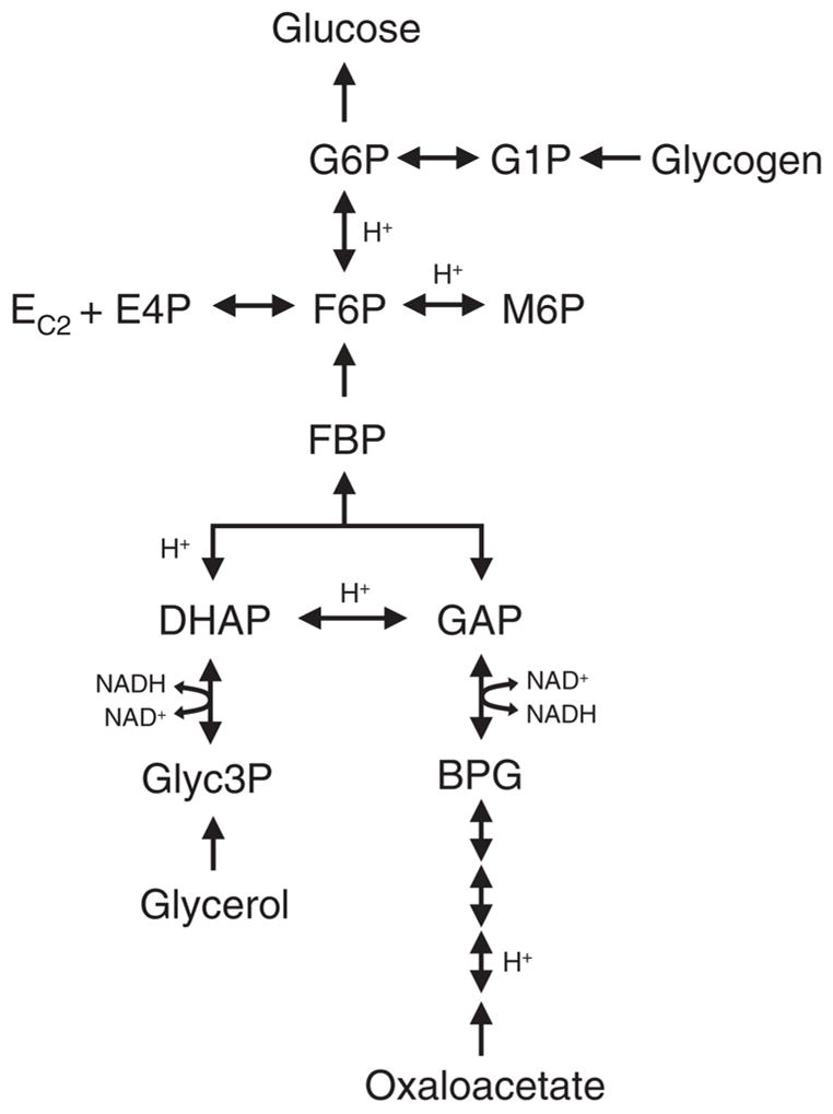
Reactions of the gluconeogenesis pathway used to simulate the labeling of glucose.

Table 9.

Metabolites in the gluconeogenesis pathway. For each metabolite we considered solely stable, i.e. carbon-bound, hydrogen atoms.

Metabolite name	Carbon atoms	Hydrogen atoms	Oxygen atoms	Total atoms
Balanced metabolites
Glucose 6-phosphate (G6P)	6	7	6	19
Fructose 6-phosphate (F6P)	6	7	6	19
Fructose 1,6-bisphosphate (FBP)	6	7	6	19
Dihydroxyacetone phosphate (DHAP)	3	4	3	10
Glyceraldehyde 3-phosphate (GAP)	3	4	3	10
1,3-Bisphosphoglycerate (BPG)	3	3	4	10
3-Phosphoglycerate (3PG)	3	3	4	10
2-Phosphoglycerate (2PG)	3	3	4	10
Phosphoenolpyruvate (PEP)	3	2	3	8
Glucose 1-phosphate (G1P)	6	7	6	19
Mannose 6-phosphate (M6P)	6	7	6	19
Glycerol 3-phosphate (Glyc3P)	3	5	3	11
Erythrose 4-phosphate (E4P)	4	5	4	13
Transketolase + C2H2O2 moiety (E-C2)	2	2	2	6
Products
Glucose	6	7	6	19
Carbon dioxide	1	0	2	3
Substrates
Oxaloacetate	4	2	5	11
Glycerol	3	5	3	11
Glycogen	6	7	6	19
NADH	0	1	0	1
Water	0	2	1	3

Table 10.

Complete list of EMUs generated for the simulation model of glucose from EMU network decomposition of the gluconeogenesis pathway. The mass isotopomer distribution of glucose, including all carbon, hydrogen, and oxygen atoms was simulated. This required only 493 EMUs (354 EMUs in the reduced model). In comparison 2,637,120 isotopomers/cumomers would have been required to describe this system.

Full EMU model		Reduced EMU model
EMU size	No. EMUs in subnetwork	EMU size	No. EMUs in subnetwork
1	11, 8	1	8, 5
2	12, 11, 9	2	9, 8, 6
3	11, 11, 11, 10, 9	3	8, 8, 8, 7, 6
4	12, 11, 11, 11, 9, 9, 9, 6, 1	4	9, 8, 8, 8, 6, 6, 6, 4, 1
5	12, 12, 11, 10, 9, 9, 9, 9, 5, 6, 1, 1, 1	5	9, 9, 8, 7, 6, 6, 6, 6, 4, 4, 1, 1, 1
6	12, 10, 10, 10, 10, 9, 9, 9, 5, 1, 1	6	9, 8, 7, 7, 7, 6, 6, 6, 4, 1, 1
7	11, 10, 10, 10, 9, 8	7	9, 7, 7, 7, 6, 6
8	10, 9, 8	8	7, 7, 6
9	9, 5	9	7, 3
10	5	10	3
11	none	11	none
12	none	12	none
13	6	13	4
14	none	14	none
15	none	15	none
16	none	16	none
17	5	17	4
18	5, 4	18	4, 4
19	6	19	4
Total number of EMUs = 493		Total number of EMUs = 354

Table 11.

Comparison of modeling approaches for simulating glucose labeling in the gluconeogenesis pathway. Different combinations of stable isotopes can be used to trace this pathway. Here, we considered ¹³C-carbon tracers, ²H-hydrogen tracers, and ¹⁸O-oxygen tracers. The total number of variables required to simulate the labeling of glucose was determined for the EMU approach and the isotopomer/cumomer methods.

	Total number of variables
Tracer used	Isotopomer/cumomer methods	EMU full model	EMU reduced model
13C	396	51	35
18O	420	88	61
2H	768	121	84
13C + 18O	21,392	142	100
13C + 2H	42,224	206	145
18O + 2H	42,416	379	268
13C + 18O + 2H	2,637,120	493	354

4. DISCUSSION

Metabolic flux analysis (MFA) provides key parameters for quantifying physiology in fields ranging from metabolic engineering to the analysis of human metabolic disease. The mathematical centerpiece of MFA is the simulation model that describes labeling dynamics under transient or stationary conditions. An important limitation of MFA as carried out via stable-isotope labeling and stable-isotope measurements is the large number of isotopomer equations that need to be solved, especially when multiple isotopic tracers are used for the labeling of the system. The isotopomer/cumomer modeling framework is a generic top-down modeling strategy. It provides the most detailed description of the labeling state of a system given by the isotopomer fractions of all metabolites. It has been the assumption that this description of a system’s labeling state is required to interpret isotope data (Wiechert and Wurzel, 2001). However, alternative modeling methods have been developed for specific isotope measurements and for specific input of labeling. For example, it is well known that fractional enrichments of carbon atoms can be simulated efficiently using atom mapping matrices, the method that was originally proposed by Zukpe and Stephanopoulos (Zupke and Stephanopoulos, 1994). More recently, Van Winden et al. (van Winden et al., 2002) developed the concept of bondomers that allows efficient simulation of NMR fine spectra and MS data without the use of isotopomers. However, the bondomer method is valid only for ¹³C-labeling experiments where a single uniformly ¹³C-labeled substrate is applied. If multiple carbon sources are present, then all substrates need to be uniformly ¹³C-labeled with the same enrichment. This requirement significantly limits the applicability of the bondomer method.

In this contribution we have developed a novel approach for modeling isotopomer distributions that significantly reduces the size of the computational problem without any loss of information. This approach is valid for any stable-isotope measurement and any labeling input. The elementary metabolite unit (EMU) framework is a bottom-up modeling approach and is based on a highly efficient decomposition algorithm that identifies the minimum amount of information that is required for isotopic simulations. We have shown that for realistic metabolic networks EMU models are orders-of-magnitude smaller than corresponding isotopomer and cumomer models, especially when multiple isotopic tracers are applied. As such, the EMU approach is the preferred method for simulating MS and NMR measurements for metabolic flux and network analysis. Important applications of the EMU method include the analysis of metabolic pathways using a combination of multiple isotopic tracers, e.g. gluconeogenesis pathway in section 3.5, and the analysis of nonstationary systems. Due to the significant model-size reduction the EMU framework allows efficient analysis of dynamic systems. For example, the time required for dynamic simulations of the E. coli network is on the order of seconds for the EMU model, compared to an hour for the corresponding cumomer model. These and other applications of the EMU approach will be explored in more detail in subsequent studies.

References

- Anderson DH. Compartmental modeling and tracer kinetics. Springer-Verlag; New York: 1983. [Google Scholar]
- Antoniewicz MR, Kelleher JK, Stephanopoulos G. Determination of confidence intervals of metabolic fluxes estimated from stable isotope measurements. Metab Eng. 2006;8:324–337. doi: 10.1016/j.ymben.2006.01.004. [DOI] [PubMed] [Google Scholar]
- Brunengraber H, Kelleher JK, Des RC. Applications of mass isotopomer analysis to nutrition research. Annu Rev Nutr. 1997;17:559–596. doi: 10.1146/annurev.nutr.17.1.559. [DOI] [PubMed] [Google Scholar]
- Hellerstein MK. In vivo measurement of fluxes through metabolic pathways: the missing link in functional genomics and pharmaceutical research. Annu Rev Nutr. 2003;23:379–402. doi: 10.1146/annurev.nutr.23.011702.073045. [DOI] [PubMed] [Google Scholar]
- Moss GP. Basic terminology of stereochemistry. Pure Appl Chem. 1996;68:2193–2222. [Google Scholar]
- Schmidt K, Carlsen KM, Nielsen J, Villadsen J. Modeling isotopomer distributions in biochemical networks using isotopomer mapping matrices. Biotechnol Bioeng. 1997;55:831–840. doi: 10.1002/(SICI)1097-0290(19970920)55:6<831::AID-BIT2>3.0.CO;2-H. [DOI] [PubMed] [Google Scholar]
- Stephanopoulos G. Metabolic fluxes and metabolic engineering. Metab Eng. 1999;1:1–11. doi: 10.1006/mben.1998.0101. [DOI] [PubMed] [Google Scholar]
- Szyperski T. Biosynthetically directed fractional 13C-labeling of proteinogenic amino acids. An efficient analytical tool to investigate intermediary metabolism. Eur J Biochem. 1995;232:433–448. doi: 10.1111/j.1432-1033.1995.tb20829.x. [DOI] [PubMed] [Google Scholar]
- Szyperski T. 13C-NMR, MS and metabolic flux balancing in biotechnology research. Q Rev Biophys. 1998;31:41–106. doi: 10.1017/s0033583598003412. [DOI] [PubMed] [Google Scholar]
- van Winden WA, Heijnen JJ, Verheijen PJ. Cumulative bondomers: a new concept in flux analysis from 2D [13C,1H] COSY NMR data. Biotechnol Bioeng. 2002;80:731–745. doi: 10.1002/bit.10429. [DOI] [PubMed] [Google Scholar]
- Wiechert W. 13C metabolic flux analysis. Metab Eng. 2001;3:195–206. doi: 10.1006/mben.2001.0187. [DOI] [PubMed] [Google Scholar]
- Wiechert W, Mollney M, Isermann N, Wurzel M, de Graaf AA. Bidirectional reaction steps in metabolic networks: III. Explicit solution and analysis of isotopomer labeling systems. Biotechnol Bioeng. 1999;66:69–85. [PubMed] [Google Scholar]
- Wiechert W, Siefke C, deGraaf AA, Marx A. Bidirectional reaction steps in metabolic networks: II. Flux estimation and statistical analysis. Biotechnology and Bioengineering. 1997;55:118–135. doi: 10.1002/(SICI)1097-0290(19970705)55:1<118::AID-BIT13>3.0.CO;2-I. [DOI] [PubMed] [Google Scholar]
- Wiechert W, Wurzel M. Metabolic isotopomer labeling systems. Part I: global dynamic behavior. Math Biosci. 2001;169:173–205. doi: 10.1016/s0025-5564(00)00059-6. [DOI] [PubMed] [Google Scholar]
- Zupke C, Stephanopoulos G. Modeling of isotope distributions and intracellular fluxes in metabolic networks using atom mapping matrices. Biotechnology Progress. 1994;10:489–498. [Google Scholar]