Exploiting noise in array CGH data to improve detection of DNA copy number change

Abstract

Developing effective methods for analyzing array-CGH data to detect chromosomal aberrations is very important for the diagnosis of pathogenesis of cancer and other diseases. Current analysis methods, being largely based on smoothing and/or segmentation, are not quite capable of detecting both the aberration regions and the boundary break points very accurately. Furthermore, when evaluating the accuracy of an algorithm for analyzing array-CGH data, it is commonly assumed that noise in the data follows normal distribution. A fundamental question is whether noise in array-CGH is indeed Gaussian, and if not, can one exploit the characteristics of noise to develop novel analysis methods that are capable of detecting accurately the aberration regions as well as the boundary break points simultaneously? By analyzing bacterial artificial chromosomes (BACs) arrays with an average 1 mb resolution, 19 k oligo arrays with the average probe spacing <100 kb and 385 k oligo arrays with the average probe spacing of about 6 kb, we show that when there are aberrations, noise in all three types of arrays is highly non-Gaussian and possesses long-range spatial correlations, and that such noise leads to worse performance of existing methods for detecting aberrations in array-CGH than the Gaussian noise case. We further develop a novel method, which has optimally exploited the character of the noise, and is capable of identifying both aberration regions as well as the boundary break points very accurately. Finally, we propose a new concept, posteriori signal-to-noise ratio (p-SNR), to assign certain confidence level to an aberration region and boundaries detected.

INTRODUCTION

Amplification or deletion of chromosomal segments can lead to abnormal mRNA transcript levels and result in the malfunctioning of cellular processes. Locating chromosomal aberrations in genomic DNA samples is an important step in understanding the pathogenesis of many diseases, most notably cancers. Microarray-based comparative genomic hybridization (array CGH) is a powerful technique for measuring such changes (1–5). To realize the promise of the array CGH technique, it is very important to develop effective methods to identify aberration regions from array CGH data. Existing analysis methods (6–23) can be roughly classified into two categories: smoothing-based (6–9) and segmentation-based (10–19). The latter approaches explicitly model the observed array data as a series of segments, with unknown boundaries and unknown heights estimated from the data by employing certain optimization criterion. While the boundary points thus identified are reliable, the aberration regions identified may be less so, in the sense that some of them may be false positives. Smoothing-based approaches assume that true signals in a specific region, aberration or non-aberration, are smoother than any kind of noise superimposed on the signals. Therefore, they attempt to reduce noise by comparing individual data points to their adjacent ones and modifying them. While such methods can reduce the number of false aberration regions identified, the boundary points detected are usually less accurate than segmentation-based methods. It would be very desirable to develop new methods for analyzing array CGH data, with both the merits of smoothing and segmentation based approaches. Such a goal may not be fully accomplished by just incorporating mean or median smoothing to a segmentation-based method.

The term ‘noise’ is often used in biology to describe experimental measurement imprecision. In particular, when evaluating the accuracy of an algorithm for detecting aberrations, it is commonly assumed that noise in the data follows normal distribution. However, this important assumption has not been verified/falsified based on the analysis of experimental data. More importantly, one has to ask whether the performance of an algorithm depends on the character of the noise, and if yes, can one exploit the characteristics of noise to improve detection of aberrations?

To address the above questions, in this work, we treat any deviations from mean values as noise. Therefore, our noise essentially represents the array CGH measurements themselves, encompassing both global measurement imprecision and localized underlying biological alterations. Based on the analysis of bacterial artificial chromosomes (BACs) arrays with an average 1 mb resolution (2), 19 k oligo arrays with the average probe spacing < 100 kb (24) and 385 k oligo arrays with the average probe spacing of about 6 kb http://www.nimblegen.com/product/cgh/, we show that when there are aberrations, noise in all three types of arrays is highly non-Gaussian and possesses long-range spatial correlations. We also show that such noise indeed leads to worse performance of existing methods for detecting aberrations in array-CGH than the Gaussian noise case. Fortunately, such noise can be exploited to devise a novel algorithm for analyzing array-CGH, which is capable of identifying both aberration regions as well as the boundary break points very accurately. We also address the fundamental question of how to assign certain confidence level to an aberration region and boundaries detected, by proposing a new concept, posteriori signal-to-noise ratio (p-SNR).

CHARACTERIZATION OF NOISE IN ARRAY CGH

In this section, we carry out distributional analysis as well as spatial correlation analysis of array-CGH noise, and assess the effect of such noise on the performance of published algorithms for detecting aberrations from array-CGH data. Below, we first describe data.

Data

In this paper, we analyze data of three resolutions, BAC array (2), 19 k oligo array (24) and 385 k oligo array http://www.nimblegen.com/product/cgh/. The BAC array (2) has an average 1 mb resolution. It is from Stanford University, which can be freely downloaded from http://www.nature.com/ng/journal/v29/n3/suppinfo/ng754_S1.html. It consisted of 15 human cell lines with known karyotypes (12 fibroblast cell lines, 2 chorionic villus cell lines and 1 lymphoblast cell line) from the NIGMS Human Genetics Cell Repository. Each cell line had been hybridized with an array CGH of 2276 BACs, spotted in triplicate. The variable used for analysis was the normalized average of the log base 2 test over reference ratio, as processed by the original authors. In each cell line, there were either one or two aberrations. Among the 15 cell lines, 6 had aberrations that covered an entire chromosome. Note that some of these datasets were recently used by Olshen and Vankatraman (12) to evaluate the effectiveness of their algorithm for detecting aberrations from the data. For convenience, the names of the 15 cell lines are listed in the first column of Table 1.

Table 1.

p-SNR and Hurst parameter for noise of the 15 BAC array data (2).

Cell line/chromosome(s)	p-SNR	H
GM01750/9/14	3.555/5.905	0.743
GM01524/6	5.308	0.739
GM01535/5/12	4.032/12.170	0.688
GM03134/8	2.829	0.619
GM03563/3/9	3.910/11.019	0.715
GM05296/10/11	5.793/3.741	0.666
GM07081/7	3.193	0.664
GM13031/17	5.172	0.667
GM13330/1/4	3.982/7.947	0.663
GM00143/18	4.429	0.741
GM02948/13	3.960	0.718
GM03576/2/21	5.080/5.473	0.770
GM04435/16/21	4.337/4.266	0.707
GM07408/20	5.774	0.712
GM10315/22	5.277	0.728

When there are two aberration regions, p-SNR is defined for both regions.

The 19 k oligo array data (24) are from Harvard Medical school. It has an average probe spacing of <100 kb. The complete OligoLibrary consists of 18 861 oligos representing 18 664 LEADSTM clusters and 197 positive controls. There are four datasets for lymphoma tumors that developed in ATM deficient mice

The 385 k oligo array data http://www.nimblegen.com/product/cgh/ has a median probe spacing of 6 000 bp through genic and intergenic regions. There are two datasets for the 385 k oligo array data. One is the normal female versus male case, where polymorphisms are observed by our method (to be described later) in chromosomes 1, 4 and 5. Another is the tumor case, where chromosome 8 has the longest aberration length (∼2000), while chromosomes 10 and 19–22 do not have detectable aberrations at all. (see Figure 1). Note that if we downsample the data to a resolution comparable to the BAC array data (2), then the longest aberration region in chromosome 8 only has less than 20 points. Therefore, the 385 k oligo array data http://www.nimblegen.com/product/cgh/ has the smallest aberration regions.

Figure 1.

The 385 k oligo array data for (a) chromosome 1, normal; (c) chromosome 1, tumor; (e) chromosome 8, normal; (g) chromosome 8, tumor. The right column ones are the corresponding data processed by the proposed method described in Exploiting noise to improve deflection of aberrations from array CGH data. The negative peak in (b) contains six sample points.

Distributional analysis of array CGH noise

When carrying out distributional analysis, an important issue to consider is the size of the sample points. For the 385 k oligo array data http://www.nimblegen.com/product/cgh/, we have considered noise for each chromosome in two scenarios, corresponding to that aberration and non-aberration regions (i) are considered together and (ii) are considered separately. The results are similar for both scenarios. For the BAC array data (2) and the 19 k oligo array data (24), we have also considered two cases, (i) each chromosome is considered separately and (ii) all the chromosomes are combined together. While the distribution for all the chromosomes combined is not the same as that for individual chromosomes, the qualitative feature of deviation from Gaussian distributions is similar for both cases. Comparisons of these different scenarios suggest that the non-Gaussian distributions discussed below may not be due to summation of multiple Gaussian distributions with different variance, corresponding to the euploid and copy-number-variant parts of the chromosome. In the main text here, we present results for the first scenario for all three types of data. Readers interested in knowing more details about the second scenario are referred to Supplementary Figures 1–3.

To simplify analysis, we have simply formed histograms. This is justified by noticing that the number of sample points is large in all the datasets. The distributions for the noise in two of the 15 BAC array data (cell line GM05296 and GM04435) are shown in Figure 2a and b. We observe that the distribution deviates from the Gaussian distribution considerably. In fact, these are typical results for the BAC array data (2). The distribution of noise in the 19 k oligo array data (24) is even more non-Gaussian, as shown in Figure 2 c,d, which are typical among the four datasets. Since the 19 k oligo array data (24) has wider aberration regions, we suspect that the deviation from Gaussian distribution is positively correlated 5 with the length of aberration regions. This hypothesis seems to be supported by analysis of the 385 k oligo array data http://www.nimblegen.com/product/cgh/. In Figure 2 e–h we have shown the distributions for noise in chromosomes 8 and 9 of both the normal and tumor cases, where Figure 2 (e and g) are for the normal case, while Figure 2 (f and h) are for the tumor case. Note that distributions for noise in other chromosomes are very similar to those shown in Figure 2 e–h. We observe that the distribution in Figure 2 (e and g) is very close to Gaussian, while the distribution in Figure 2 (f and h) is non-Gaussian, but the deviation from Gaussian is less severe than that shown in Figure 2 (a–d). Note that there are no aberrations in the normal case, while the aberration region in the tumor case of the 385 k oligo array data http://www.nimblegen.com/product/cgh/ are smaller than those in the BAC array data (2).

Figure 2.

Probability distribution function (PDF) for noise of (a,b) BAC array data (cell line GM05296 and GM04435), (c,d) 19k oligo array data, (e) 385k oligo array data, chromosome 8, normal case, and (f) 385k oligo array data, chromosome 8, tumor case, (g) 385k oligo array data, chromosome 9, normal case, and (h) 385k oligo array data, chromosome 9, tumor case. The solid black curves are estimated from the data, while the dashed red ones are the fitted Gaussian distribution curves.

Spatial correlations in array CGH noise

Denote array CGH noise by x₁,x₂,⋯x_t and the spatial resolution by Δx. We have found that array CGH noise can be characterized as a type of fractal noise characterized by an algebraically decaying spatial autocorrelation function,

1

where m corresponds to physical spacing mΔx, 0 < H < 1 is the Hurst parameter (25). In particular, when 1/2 < H < 1, the summation of the autocorrelation becomes unbounded if m can go to infinity. Therefore, such noise process is often said to have long-range persistent correlations. We shall discuss its implications to DNA copy number change momentarily. When H = 1/2, the noise is like the white Gaussian noise.

There exist many different ways to estimate the Hurst parameter H (25,26). For ease of interpretation, we choose variance-spacing relation. To use this method, one can analyze non-overlapping running means of the original array data by constructing a new time series t = 1, 2, 3, }, m = 1, 2, 3, ···:

For a noise process with the property described by Equation (1), the variance of the running means, , declines in a power-law manner as the size of the sample, m, increases:

2

where σ² is the variance of the original time series x_t. Based on Equation (2), one can readily understand the meaning of H in terms of how effective smoothing can reduce variations in the noise. For example, when H = 0.5, var(X^(m)) drops to σ²/10 when m = 10. However, if H becomes 0.75, then for the variance to drop to σ²/10, one needs to take m = 100. This is an order of magnitude larger than if H = 0.5. In other words, smoothing is less effective in reducing variations in the data. For notational convenience, we shall re-write Equation (2) as

3

We examine the long-range spatial correlations in the 385 k oligo array data http://www.nimblegen.com/product/cgh/ first. Since the datasets have very high-spatial resolution, in each chromosome, we have plenty of data points. We carry out variance-spacing relation analysis of the data in each chromosome separately. When aberration regions exist in the data, we pre-process the data using two methods. One is to discard the part of data corresponding to the aberration regions. Another is to retain the part of data corresponding to the aberration regions, with the mean of that part removed. It is clear that after processing by either method, the remaining data is the fluctuations or noise in the array probes. The characteristics of fluctuations by both methods are similar. Below, we present results for the first method. Figure 3 shows log₂ F(m) vs. log₂ m for the data of the six chromosomes of the 385 k oligo array data, where the red diamond is for the tumor case, while the black circle is for the normal case. The solid black and dashed red lines are straight lines fitted by linear least squares regression, whose slopes estimate the Hurst parameter. We observe that the fitted straight lines are valid up to m = 2¹⁰. Since the spatial resolution of the data are ∼6 kb, this corresponds to ∼6 Mb physical spacing within the chromosome. We also observe that for the chromosomes 1, 8, 9 and 12, which have fairly large aberration regions, the Hurst parameters for the tumor case are larger than those for the normal case. In fact, in the tumor case, those Hurst parameters are much larger than 0.5, indicating strong long-range spatial correlations. However, for the chromosomes 19 and 20, which do not have any aberration regions, there is little difference in the Hurst parameter between the tumor and the normal case.

Figure 3.

log₂F(m) versus log₂ m for the data of the 6 chromosomes of the 385 k oligo array datasets. The red diamond is for the tumor case, while the black circle is for the normal case. The solid black and dashed red lines are straight lines fitted by linear least squares regression. There are no aberrations in chromosomes 19 and 20. The Hurst parameters are obtained as the slopes of the straight lines, which are indicated in the figure.

Comparing spatial correlation analysis with distributional analysis of the 385k oligo array data http://www.nimblegen.com/product/cgh/, we make a few interesting observations. In terms of distributions, all the chromosomes are similar: the distributions are close to Gaussian in the normal case (Figure 2e and g) but deviate, with similar degree, from Gaussian in the tumor case (Figure 2f and h). In terms of spatial correlations, chromosomes with aberrations are characterized by a Hurst parameter larger than 0.5 (Figure 3a–d), indicating array probes to be correlated with array probes not only nearby but also far away. Because of this, different chromosomes in the tumor case become different, depending on whether there are aberrations in the chromosomes, and if yes, how large the aberration regions are. On the other hand, chromosomes without aberrations become all similar, irrespective of whether they are in the normal or tumor case. Therefore, spatial correlation is a better means to characterize aberrations than the distribution.

Due to the low spatial resolution of the BAC array data (2) and the 19 k oligo array data (24), in each chromosome, we do not have enough data points to carry out variancespacing relation analysis. Thus, we have performed the analysis based on the whole array data, without separating the data into different chromosomes. We find that the Hurst parameters for the BAC array data (2) and the 19 k oligo array data (24) are in the range of 0.6–0.77 (H for the BAC array data (2) are listed in the 3rd column of Table 1). While they are all larger than 0.5, suggesting long-range spatial correlations, we have to emphasize that such long-range spatial correlations are the correlations across chromosomes, and therefore, are different than the correlations in the 385 k oligo array data http://www.nimblegen.com/product/cgh/, which are within chromosomes. We believe this is the primary reason that the Hurst parameters for the BAC array data (2) and the 19 k oligo array data (24) are smaller than those of the 385 k oligo array data http://www.nimblegen.com/product/cgh/ with tumors. While the long-range spatial correlations in the BAC array data (2) and the 19 k oligo array data (24) might not have much biological relevance, they are important features to consider when one designs methods to detect DNA copy number changes from them.

Effect of array noise on detection of aberrations

To illustrate the effect of array noise on detection of aberrations, we choose CGHseg algorithm (15), which is one of the best segmentation based algorithms, and consider simulated data of various aberration widths (5, 10, 20 and 40 probes) and noise levels (SNR of 1, 2, 3 and 4). SNR is defined as the mean magnitude of the aberration (i.e. signal) divided by the SD of the superimposed noise. Two types of noise are considered. One is simulated Gaussian noise. The other is the actual noise in the BAC array data (2). For each aberration width and SNR, we generate 100 artificial chromosomes, each consisting of 100 probes and with the square-wave signal profile added to the center of the chromosome. To generate receiver operating characteristic (ROC) curve corresponding to a particular aberration width and SNR, we calculate the true positive rates (TPR) and the false positive rates (FPR). TPR is defined as the number of probes inside the aberration whose fitted values are above the threshold level divided by the number of probes in the aberration. FPR is defined as the number of probes outside the aberration whose fitted values are above the threshold level divided by the total number of probes outside the aberration. We vary the threshold value for aberration from the minimum log-ratio value to the maximum. Each threshold value results in a TPR and a FPR, represented by a point on the ROC curve. Similar simulation procedure has been used by Lai et al. (23). Figure 4 shows the ROC curves corresponding to different aberration widths and SNRs, where the purple curves correspond to the simulation with real array noise, while the green curves correspond to the simulation with Gaussian noise. We observe that the green curves are generally above the purple ones. This is especially so when SNR = 1 and the aberration width is 20. Therefore, we can conclude that performance of CGHseg algorithm for detecting aberrations from array CGH data are worse when real array noise is used than when Gaussian noise is used. Interestingly, other existing methods behave similarly.

Figure 4.

ROC curves corresponding to different aberration widths and SNRs

Summary

Summarizing the results discussed so far, we can conclude that when there are aberrations, noise in array CGH is highly non-Gaussian and possesses long-range spatial correlations. It appears that the non-Gaussian feature as well as the long-range spatial correlation feature become stronger when the aberration regions become larger. When SNR is low and the aberration width is large, performance of existing methods for detecting aberrations is worse with this type of noise than when noise is assumed to be Gaussian.

EXPLOITING NOISE TO IMPROVE DETECTION OF ABERRATIONS FROM ARRAY CGH DATA

We now present an algorithm for detecting aberrations from array CGH data that has considerably taken into account the character of array noise. Since the method has merits of both smoothing and segmentation based methods, we denote it by CGHss. It consists of five steps. They are detailed below.

1. To reduce noise, the original log₂ ratio data y(n), n = 1,2,⋯,N is filtered by a median filter. In order not to lose too much information about the boundary, the length of the filter is 3-point. Let us denote the resulting data by y₁(n).

2. Construct a random walk process from y₁(n) by simply forming partial summation of y₁(n) based on the following formula,

   4

   where μ is the mean of y₁(n); then is partitioned into overlapping segments of length 3 and overlap 2, and the local trend in each segment is calculated to be the ordinate of a linear least-squares fit for the random walk in that segment. Denote the difference between the original walk and the local trend by y₂(n).

   Note this step plays the role of smoothing. In particular, as will be shown in Figure 5c, the pattern of can be well associated with the aberration regions. We emphasize that unlike conventional lossy smoothing, here, information on original data can be recovered. Hence, it is a lossless smoothing. Furthermore, y₂(n) can be used to estimate the Hurst parameter through the method called detrended fluctuation analysis (28). Therefore, this is the step that has fully taken into account the spatial correlation feature of the data.

3. Let var{a,b} denote the variance of two variables a and b, which is simply (a − b)²/2. Now we modify y₁(n) according to the following rule:

   5

   Note this step does both segmentation and smoothing.
4. Let

   

   and define

   6

   where T₁ is a threshold value. This step yields a square wave-like signal. With this signal, we can make simple decisions, which is our step (5).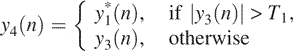

5. Set thresholds T₂ (a positive number) and T₃ (a negative number), and identify the regions in y₄(n) data greater than T₂ or less than T₃ as potential amplifications or deletions in array CGH data. Sometimes in order to reduce false positives, we may discard small regions with only one or two probes. However this should be done with caution, since some microdeletions may only contain a single probe.

Figure 5.

A schematic figure illustrating the proposed method. (a) shows the original array data, (b-g) show the signals y₁(n), , y₂(n), , y₃(n) and y₄(n), respectively. The dashed red lines in (f) denote the threshold T₁.

To make the above steps concrete, we have simulated an artificial chromosome data consisting of 100 probes, with the centering 10 probes having aberrations. The simulated data y(n) is shown in Figure 5a. Figure 5b–g show the signals y₁(n), , y₂(n), , y₃(n) and y₄(n), respectively. The red dashed lines in Figure 5f correspond to a more or less arbitrarily chosen threshold value T₁.

Note all the three thresholds, T₁, T₂ and T₃, can be defined by users. Also note that the ROC curves presented below do not depend on T₁ sensitively. After we describe the concept of p-SNR, we shall provide some guidelines as how to choose T₂ and T₃.

We now compute the ROC curves for our method under the same setting as when we discussed the CGHseg algorithm (Figure 4, green and purple curves). They are shown in Figure 4 as red and black curves, for array noise and Gaussian noise, respectively. First we note that comparing with the results of a recent comparison paper (23), our method is comparable to the best smoothing based methods. Next, we make two interesting observations from Figure 4 (i) The ROC curves for our method are very similar for the array noise and the Gaussian noise. This is because our method has fully taken into account the character of the array noise. (ii) Our method is more accurate than CGHseg, especially when SNR is low and the aberration width is narrow. As we shall argue later, in the low SNR case, a good threshold to choose would correspond to the case of TPR + FPR =1 = 1. Under such a criterion, our method is almost 20% more accurate than CGHseg, for the case of SNR = 1 and aberration width = 5. Therefore, our method will be especially useful for processing array CGH data with small SNR [the 19 k oligo array data (24) belong to this category, as we shall show in the next section].

Next we examine the performance of our method for detecting the boundaries of aberrations. Figure 6 compares our result with those obtained using the CGHseg algorithm (15) The simulated data, shown in Figure 6a, consists of a single aberration region, from 48 to 52. Due to fairly low SNR, visually it is hard to tell which region might be the aberration region. However, our method correctly detects both the aberration region and the two breakpoints, as shown in Figure 6b. The CGHseg algorithm, however, does not seem to be able to cope with such low SNR data. This is evident in Figure 6(c and d) (as well as Supplementary Figures 4–7): The CGHseg method may not only produce false aberration regions, but also fail to detect boundary points correctly. The reason that our method works better is that a few steps of our method have used smoothing. In particular, the second step of our method is a lossless smoothing. No other methods have done so.

Figure 6.

Comparison of our result with those obtained using CGHseg algorithm (15). The aberration region consists of 5 probes, from 48 to 52. SNR is 2. (a) shows the simulated data; this signal is also shown in (b–d) as blue dots. (b) shows the result of our method. The red curve is y₄(n), as explained in the procedure. The breakpoints 48 and 52 are both correctly detected; (c) shows the result by CGHseg algorithm using heteroscedastic model, the estimated number of segments is K = 3, while the breakpoints identified are 65 and 66; (d) shows the result by CGHseg algorithm using homoscedastic model. The estimated number of segments is K = 8, one of the two breakpoints, 48, is correctly detected. In (c and d), red lines represent the estimated mean of each segment, and green lines, the estimated mean plus or minus 1SD. To aid visual inspection, vertical dotted lines are drawn in (b–d).

Finally, we evaluate our method by analyzing 15 BAC array data (2). Figure 7 compares aberration detection by using Figure 7a and b our method and Figure 7c and d the method of Olshen and Vankatraman Olshen (12) The cell line is GM05296, with known aberrations on chromosomes 10 and 11. We observe that the two methods perform similarly well. As will be explained later, these two datasets have fairly high SNR, and hence, aberration detection is not too difficult.

Figure 7.

Aberration detection using (a,b) our method and (c,d) the method of Olshen and Vankatraman (12). The cell line is GM05296, with known aberrations on chromosomes 10 and 11. The dotted points are the original data. Red lines in (a,b) are the y₄(n) signals explained in the procedure. They represent the estimated mean of each segment in (c,d). To aid visual inspection, vertical dotted lines are drawn in all the plots.

POSTERIORI SIGNAL-TO-NOISE-RATIO (P-SNR)

We now consider an important question: after one applies an algorithm to identify aberration regions and breakpoints from an array CGH data, how much confidence can one have on the final result? When there are a lot of data available, together with information on the background normal situations, one may follow the procedure discussed by Wang et al. Wang et al. (19). Here, we consider the more challenging case of only one array data are available.

Our solution is quite simple. It amounts to utilizing the information summarized by ROC curves obtained by numerical simulations as much as possible. From Figure 4, it is clear that the accuracy of detection depends on two critical parameters, the size of the aberration region and SNR. In fact, from Figure 4, it is clear that SNR is even more important than the size of the aberration region. Therefore, a good starting point would be to estimate SNR after one identifies one or a few aberration regions. This can be achieved by using the following simple formula:

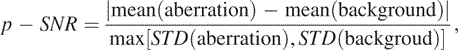7

where p is used to emphasize that this is a posteriori estimation, and mean and STD denote mean and SD of the data in the aberration region and background region (i.e. non-aberration region), respectively. When there are multiple aberration regions, p-SNR may be estimated for each aberration region identified. When this is the case, one needs to take the background region to be only around that aberration region. The p-SNR for the BAC array data (2) are listed in the second column of Table 1. We observe that they are quite large, indicating that one can have high-confidence in the final detection results for the BAC array data (2). The p-SNR for the 385 k oligo array data http://www.nimblegen.com/product/cgh/ are around 0.9 to 1.5, and are even smaller for the 19 k oligo array data (24) (around 0.7–1.1). In particular, we have estimated the p-SNR for the 385 k and 19 k oligo array data based on the X chromosome using sex-mismatched samples. We have found that the p-SNR for the two array platforms are 1.26 and 1.03, respectively, both falling in the range for each type of data listed above. Although we do not have access to the sex-mismatched X chromosome data for the BAC array data (2), based on our analysis of the other two types of data, we have good reason to believe that the p-SNR for the BAC array data's sex-mismatched X chromosome would be at least around 3, therefore, much larger than the p-SNR of the other two types of data.

Our concept of p-SNR suggests that a good starting point to choose the parameters T₂ and T₃ used in step (5) of our algorithm may correspond to signal intensity divided by p-SNR. This amounts to choosing one SD of the data. This rule suggests an iterative operation: starting from arbitrarily chosen T₂ and T₃, calculate the corresponding p-SNR, then use the criterion discussed above to obtain a new estimate of T₂ and T₃, finally calculate the new p-SNR′. If p-SNR and p-SNR′ are similar, then the two parameters have been chosen appropriately.

We emphasize that our method works excellently if p-SNR is high. However, if p-SNR is low, then one may choose threshold values that roughly yield TPR + FPR = 1, where TPR and FPR define the ROC curve. In this case, however, one should bear in mind that the classification may be incorrect with a probability of FPR.

DISCUSSION

In this paper, we have examined noise in array CGH data of three resolution, the BAC array data, the 19 k and 385 k oligo array data, and found that noise is highly non-Gaussian and possesses long-range spatial correlations. We have also developed a novel method for processing array CGH data. The method is a suitable combination of smoothing and segmentation, and has fully taken into account the characteristics of noise in array CGH data. We have shown that the method is as accurate as the best smoothing-based methods for detecting aberration regions, and as accurate as the best segmentation-based methods for finding boundary points. Furthermore, we have proposed a new concept, (p-SNR), to quantify the confidence level of aberration regions and boundaries detected. We have found that p-SNR for the 15 publicly available BAC array CGH data are all quite large, indicating it is a relatively easy matter to accurately detect aberrations and boundaries from those data. However, p-SNR for the four 19k oligo array data are quite small, suggesting it is considerably more challenging to detect aberrations from such array CGH data.

Although we have found that array CGH noise is highly non-Gaussian with long-range spatial correlations, we do not clearly know the mechanisms. A challenging task for future research would be to understand the biological mechanisms of such noise, as well as understand whether those mechanisms are differentially related to different types of diseases.

Being able to identify smaller copy-number changes that affect only a few probes is of particular importance in the field of copy number polymorphism. This is because inherited, germ-line copy number variants are typically much smaller than rearrangements in cancer genomes. For example, two recent papers, one by McCarroll et al. (29), another by Conrad et al. (30), identified a large class of inherited, multikilobase deletion polymorphisms that are predominantly smaller than 20 kb in size. We emphasize that in order to detect small copy number changes, the key is to improve the resolution of the array technology so that at least 2 points can be sampled for the region of interest. If only a single isolated point can be sampled, then it would be impossible by any analysis method to classify it as a true copy number change or just an outlier or noise.

Finally, readers interested in this method are strongly encouraged to contact with the authors (e.g. gao@ece.ufl.edu) to obtain the source Matlab code.

REFERENCES

- 1.Pinkel D, Segraves R, Sudar D, Clark S, Poole I, Kowbel D, Collins C, Kuo WL, Chen C, Zhai Y. High resolution analysis of DNA copy number variation using comparative genomic hybridization to microarrays. Nature Genet. 1998;20:207–211. doi: 10.1038/2524. [DOI] [PubMed] [Google Scholar]
- 2.Snijders AM, Nowak N, Segraves R, Blackwood S, Brown N, Conroy J, Hamilton G, Hindle AK, Huey B, Kimura K. Assembly of microarrays for genome-wide measurement of DNA copy number. Nature Genet. 2001;29:263–264. doi: 10.1038/ng754. [DOI] [PubMed] [Google Scholar]
- 3.Solinas-Toldo S, Lampel S, Stilgenbauer S, Nickolenko J, Benner A, Dohner H, Cremer T, Lichter P. Matrixbased comparative genomic hybridization: biochips to screen for genomic imbalances. Genes Chromosomes Cancer. 1997;20:399–407. [PubMed] [Google Scholar]
- 4.Ishkanian AS, Malloff CA, Watson SK, DeLeeuw RJ, Chi B, Coe BP, Snijders A, Albertson DG, Pinkel D, Marra MA. A tiling resolution DNA microarray with complete coverage of the human genome. Nature Genet. 2004;36:299–303. doi: 10.1038/ng1307. [DOI] [PubMed] [Google Scholar]
- 5.Pinkel D, Albertson DG. Array comparative genomic hybridization and its applications in cancer. Nature Genet. 2005;37 doi: 10.1038/ng1569. [DOI] [PubMed] [Google Scholar]
- 6.Pollack JR, Sorlie T, Perou CM, Rees CA, Jeffrey SS, Lonning PE, Tibshirani R, Botstein D, Borresen-Dale A-L, Brown PO. Microarray analysis reveals a major direct role of DNA copy number alteration in the transcriptional program of human breast tumors. Proc. Natl Acad. Sci. USA. 2002;99:12963–12968. doi: 10.1073/pnas.162471999. [DOI] [PMC free article] [PubMed] [Google Scholar]
- 7.Beheshti B, Braude I, Marrano P, Thorner P, Zielenska M, Squire JA. Chromosomal localization of DNA amplifications in neuroblastoma tumors using cDNA microarray comparative genomic hybridization. Neoplasia. 2003;5:53–62. doi: 10.1016/s1476-5586(03)80017-9. [DOI] [PMC free article] [PubMed] [Google Scholar]
- 8.Hsu L, Self SG, Grove D, Randolph T, Wang K, Delrow JJ, Loo L, Porter P. Denoising array-based comparative genomic hybridization data using wavelets. Biostatistics. 2005;6:211–226. doi: 10.1093/biostatistics/kxi004. [DOI] [PubMed] [Google Scholar]
- 9.Eilers PHC, de Menezes RX. Quantile smoothing of array CGH data. Bioinformatics. 2005;21:1146–1153. doi: 10.1093/bioinformatics/bti148. [DOI] [PubMed] [Google Scholar]
- 10.Hodgson G, Hager JH, Volik S, Hariono S, Wernick M, Moore D, Nowak N, Albertson DG, Pinkel D, Collins C, et al. Genome scanning with array CGH delineates regional alterations in mouse islet carcinomas. Nature Genet. 2001;29:459–464. doi: 10.1038/ng771. [DOI] [PubMed] [Google Scholar]
- 11.Jong K, Marchiori E, Meijer G, Vaart AVD, Ylstra B. Breakpoint identification and smoothing of array comparative genomic hybridization data. Bioinformatics. 2004;20:3636–3637. doi: 10.1093/bioinformatics/bth355. [DOI] [PubMed] [Google Scholar]
- 12.Olshen AB, Venkatraman ES, Lucito R, Wigler M. Circular binary segmentation for the analysis of array-based DNA copy number data. Biostatistics. 2004;5:557–572. doi: 10.1093/biostatistics/kxh008. [DOI] [PubMed] [Google Scholar]
- 13.Hupe P, Stransky N, Thiery J-P, Radvanyi F, Barillot E. Analysis of array CGH data: from signal ratio to gain and loss of DNA regions. Bioinformatics. 2004;20:3413–3422. doi: 10.1093/bioinformatics/bth418. [DOI] [PubMed] [Google Scholar]
- 14.Daruwala R-S, Rudra A, Ostrer H, Lucito R, Wigler M, Mishra B. A versatile statistical analysis algorithm to detect genome copy number variation. Proc. Natl Acad. Sci. USA. 2004;101:16292–16297. doi: 10.1073/pnas.0407247101. [DOI] [PMC free article] [PubMed] [Google Scholar]
- 15.Picard F, Robin S, Lavielle M, Vaisse C, Daudin J-J. A statistical approach for array CGH data analysis. BMC Bioinformatics. 2005;6:27. doi: 10.1186/1471-2105-6-27. [DOI] [PMC free article] [PubMed] [Google Scholar]
- 16.Autio R, Hautaniemi S, Kauraniemi P, Yli-Harja O, Astola J, Wolf M, Kallioniemi A. CGH-Plotter: MATLAB toolbox for CGH-data analysis. Bioinformatics. 2003;19:1714–1715. doi: 10.1093/bioinformatics/btg230. [DOI] [PubMed] [Google Scholar]
- 17.Myers CL, Dunham MJ, Kung SY, Troyanskaya OG. Accurate detection of aneuploidies in array CGH and gene expression microarray data. Bioinformatics. 2004;20:3533–3543. doi: 10.1093/bioinformatics/bth440. [DOI] [PubMed] [Google Scholar]
- 18.Lingjaerde OC, Baumbusch LO, Liestol K, Glad IK, Borresen-Dale A-L. CGH-Explorer: a program for analysis of array-CGH data. Bioinformatics. 2005;21:821–822. doi: 10.1093/bioinformatics/bti113. [DOI] [PubMed] [Google Scholar]
- 19.Wang P, Kim Y, Pollack J, Narasimhan B, Tibshirani R. A method for calling gains and losses in array CGH data. Biostatistics. 2005;6:45–58. doi: 10.1093/biostatistics/kxh017. [DOI] [PubMed] [Google Scholar]
- 20.Snijders AM, Fridlyand J, Mans DA, Segraves R, Jain AN, Pinkel D, Albertson DG. Shaping of tumor and drug-resistant genomes by instability and selection. Oncogene. 2003;22:4370–4379. doi: 10.1038/sj.onc.1206482. [DOI] [PubMed] [Google Scholar]
- 21.Sebat J, Lakshmi B, Troge J, Alexander J, Young J, Lundin P, Maner S, Massa H, Walker M, Chi M, et al. Large-scale copy number polymorphism in the human genome. Science. 2004;305:525–528. doi: 10.1126/science.1098918. [DOI] [PubMed] [Google Scholar]
- 22.Fridlyand J, Snijders AM, Pinkel D, Albertson DG, Jain A. Hidden Markov models approach to the analysis of array CGH data. J Multivariate Anal. 2004;90:132–153. [Google Scholar]
- 23.Lai WR, Johnson MD, Kucherlapati R, Park PJ. Bioinformatics. 2005. Comparative analysis of algorithms for identifying amplifications and deletions in array CGH data. [DOI] [PMC free article] [PubMed] [Google Scholar]
- 24.Ziv S, Brenner O, Amariglio N, Smorodinsky NI, Galron R, Carrion DV, Zhang WJ, Sharma GG, Pandita RK, et al. Impaired genomic stability and increased oxidative stress exacerbate different features of Ataxia-telangiectasia. Hum. Mol. Genet. 2005;14:2929–2943. doi: 10.1093/hmg/ddi324. [DOI] [PubMed] [Google Scholar]
- 25.Mandelbrot BB. The Fractal Geometry of Nature. San Francisco: Freeman; 1982. [Google Scholar]
- 26.Gao JB, Hu J, Tung WW, Cao YH, Sarshar N, Roychowdhury VP. Assessment of long range correlation in time series: How to avoid pitfalls. Phys. Rev. E. 2006;73:016117. doi: 10.1103/PhysRevE.73.016117. [DOI] [PubMed] [Google Scholar]
- 27.Gao JB, Billock VA, Merk I, Tung WW, White KD, Harris JG, Roychowdhury VP. Inertia and memory in ambiguous visual perception. Cogn. Process. 2006;7:105–112. doi: 10.1007/s10339-006-0030-5. [DOI] [PubMed] [Google Scholar]
- 28.Peng CK, Buldyrev SV, Havlin S, Simons M, Stanley HE, Goldberger AL. Mosaic organization of dna nucleotides. Phys. Rev. E. 1994;49:1685–1689. doi: 10.1103/physreve.49.1685. [DOI] [PubMed] [Google Scholar]
- 29.McCarroll SA, Hadnott TN, Perry GH, Sabeti PC, Zody MC, Barrett JC, Dallaire S, Gabriel SB, Lee C, Daly MJ, Altshuler DM. Common deletion polymorphisms in the human genome. Nature Genet. 2006;38:86–92. doi: 10.1038/ng1696. [DOI] [PubMed] [Google Scholar]
- 30.Conrad DF, Andrews TD, Carter NP, Hurles ME, Pritchard JK. A high-resolution survey of deletion polymorphism in the human genome. Nature Genet. 2006;38:75–81. doi: 10.1038/ng1697. [DOI] [PubMed] [Google Scholar]