Anatomical constraints on source models for high-resolution EEG and MEG derived from MRI

Abstract

Electroencephalography (EEG) remains the primary tool for measuring changes in dynamic brain function due to disease state with the millisecond temporal resolution of neuronal activity. In recent decades EEG has been supplanted by CT and MRI for the localization of tumors and lesions in the brain. In contrast to the excellent temporal resolution of EEG, the spatial information in EEG is limited by the volume conduction of currents through the tissues of the head. We have extracted source models (position and orientation) from MRI scans to investigate the theoretical relationship between brain sources and EEG recorded on the scalp. Although detailed information about the boundaries between different tissues can also be obtained from MRI, these models are only approximate because of our relatively poor knowledge of the conductivities of the different tissue compartments in living heads. We also compare the resolution of EEG with magnetoecephalography (MEG) which offers the advantage of requiring less detail about volume conduction in the head. The brain’s magnetic field depends only on the position of sources in the brain and the position and orientation of the sensors. We demonstrate that EEG and MEG space average neural activity over comparably large volumes of the brain; however, they are preferentially sensitive to sources of different orientation suggesting a complementary role for EEG and MEG. High-resolution EEG methods potentially yield much better localization of source activity in superficial brain areas. These methods do not make any assumptions about the sources, and can be easily co-registered with the brain surface derived from MRI. While there is much information to be gained by using anatomical MRI to develop models of the generators of EEG/MEG, functional neuroimaging (e.g., fMRI) signals and EEG/MEG signals are not easily related.

Introduction

Electroencephalography (EEG) is widely used in the diagnosis and monitoring of epilepsies, including epilepsies associated with brain tumors. Historically, EEG also served as a diagnostic tool for detecting brain tumors. In 1936, Grey Walter, who introduced the term “delta waves,” first identified the association between excessive slow waves (< 2 Hz) and tumors of the cerebral hemispheres (1). The foci of the abnormal delta waves typically overlays the underlying area of cerebral infarct (2–3). The role of EEG in detecting focal tumors and lesions has been supplanted by CT and MRI. Today, EEG is used primarily to complement these studies by assessing dynamic brain function. In particular, EEG can be used to evaluate the effects of tumor or lesion on surrounding tissue and distant brain areas that are functionally coupled to that region.

EEG is a very large-scale measure of brain source activity, apparently recording synaptic activity synchronized over macroscopic (centimeter), regional, and even whole brain spatial scales (4–5). The inherent complexity of the spatiotemporal dynamics of EEG indicates that conceptual models that view source activity as consisting of only one source region are inadequate. Synchrony among neural populations in compact regions of the brain produces localized dipole current sources. Synchrony among dipole sources distributed across the cortex can give rise to regional or global sources. EEG reflects this brain source activity, of unknown spatial extent, that has been spatially filtered by the volume conduction of currents through the head.

The existence of localized generators is apparently not a general property of EEG data

The objective of any realistic source analysis is to characterize EEG sources without making prior assumptions about the actual nature of the sources. In some cases, such as short latency sensory evoked potentials or epileptic discharges, the assumption that a single focal region of the cortex is the main EEG generator may be used to justify modeling signals with a single dipole source. However, in general, EEG signals can evidently be generated regionally or even globally, involving neural populations acting in concert. EEG signals related to cognitive processes probably involve distributed cortical tissue, perhaps in multiple, widely separated brain regions. A mixture of local, regional, and global sources is a more useful picture of the sources of EEG (3).

MEG (magnetoencephalography) is a relatively new technology that provides useful insights into brain sources when used as an adjunct to EEG measurements. The small magnetic field generated by brain sources can be recorded 1–2 cm above the scalp by SQUID (Superconducting Quantum Interference Device) coils, using either single coils (magnetometers) or pairs of coils (gradiometers). MEG is two orders of magnitude more expensive than EEG, which has limited its adoption in both cognitive and clinical studies. One common but entirely erroneous idea is that MEG spatial resolution is inherently superior to EEG spatial resolution, and that MEG should simply replace EEG in order to extract more accurate information about sources. MEG and EEG are selectively sensitive to different sources; this can be either an advantage or disadvantage of MEG, depending on application. The main advantage of MEG is that far less detailed information about the tissues of the head is required to model the generators.

In this paper, anatomical information from MRI is used to model the sources underlying EEG and MEG signals. MRI based models of the cortex are used to demonstrate the EEG and MEG are largely sensitive to different sources. Estimates of the boundaries between tissues with different conductivity, specifically the brain, skull, and scalp, can also be obtained from MRI and incorporated into a boundary element model (BEM) of the head. However, because of limitations in our knowledge of tissue conductivity, it is not at all clear that these models represent a significant improvement over spherical and ellipsoidal models that assume uniform layers. High-resolution EEG methods are a model independent approach to detect the sources of EEG signals based on spatial filtering. By combining high-resolution EEG methods with source models derived from MRI, detailed estimates of superficial cortical sources can be obtained from EEG.

Methods

Dipole sources of EEG and MEG

The dipole approximation to cortical current sources provides the basis for any realistic source model of EEG or MEG. It is based on the idea that at large distances, any complex current distribution in a small region of the cortex can be approximated by a “dipole” or more accurately, a dipole moment per unit volume (5). A “large” distance in this case is at least 3 or 4 times the distance between the effective poles of the dipole. Superficial gyral surfaces are located at roughly 1.5–2 cm from scalp electrodes, separated by a thin layer of cerebrospinal fluid (CSF), skull, and scalp. In this context, the dipole approximation appears valid only for superficial cortical tissue with a maximum extent in any dimension of roughly 0.5 cm or less. Macrocolumns (approximately 3 mm diameter) provide a convenient scale to picture dipoles. This spatial scale is sufficiently large that synaptic sources within the volume will be approximately balanced by sinks within the volume (eliminating monopolar source terms) and small enough to be approximated by a dipole. However, the word “dipole” is actually just convenient jargon for dipole moment per unit volume P(r, t), which is a space-average of synaptic sources (5). The strength of the dipole moment depends not only on the strength of the individual sources, but also their spatial distribution within the tissue mass, for instance by the concentration of positive and negative sources in different cortical layers.

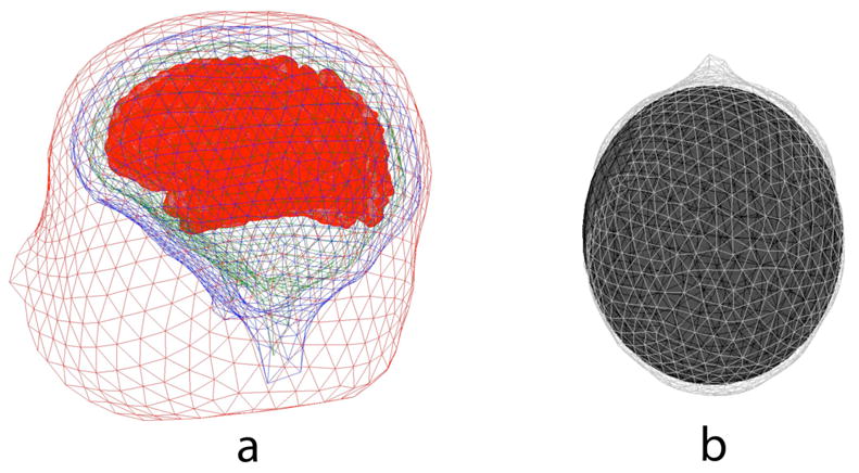
With this definition, there can be multiple active dipole sources within a 2 cm² gyral crown; that is, the crown forms a small dipole layer. The sources of many (if not most) EEG and MEG signals may then be pictured as tens of thousands cortical dipoles, mainly oriented perpendicular to the cortical surface forming dipole layers (or folded dipole sheets), as depicted pictorially in Fig. 1a. The EEG electrode affixed to the scalp in Figure 1a measures the scalp potential with reference to another electrode (not shown); the MEG sensor in free space measures the component of the magnetic field that passes through the coil. At any location in the cortex, the dipole moment is a vector indicating separate strengths in three orthogonal directions. However, approximately 85% of neurons are pyramidal cells oriented perpendicular to the cortical surface (6). Thus, the moment normal to the cortex is expected to be strongest suggesting that dipole orientation can be approximated from the cortical geometry. EEG is most sensitive to correlated dipole layer in gyri (regions ab, de, gh), less sensitive to correlated dipole layer in sulcus (region hi) and insensitive to opposing dipole layer in sulci (regions bcd, efg) and random layer (region ijklm). MEG is most sensitive to correlated and minimally opposed dipole layer (hi) and much less sensitive to all other sources shown, which are opposing, random or radial dipoles.

Figure 1.

Sources of EEG and MEG. a. Neocortical sources can be generally pictured as dipole layers (or “dipole sheets”, in and out of cortical fissures and sulci) with meso-source strength varying as a function of cortical location. EEG is most sensitive to correlated dipole layer in gyri (regions ab, de, gh), less sensitive to correlated dipole layer in sulcus (region hi) and insensitive to opposing dipole layer in sulci (regions bcd, efg) and random layer (region ijklm). MEG is most sensitive to correlated and minimally apposed dipole layer (hi) and much less sensitive to all other sources shown, which are opposing, random or radial dipoles. b. Source model obtained by segmenting MRI images (left hemisphere shown). The source model consists of more than 10⁶ vertices. The sources are assumed normal to the cortical surface.

These considerations provide very strong motivation for making use of MRI to determine the locations and orientation of brain sources. Figure 1b shows a source model consisting of around a hundred thousand dipoles for each hemisphere. The brain surface geometry was obtained by a combination of automated and manual segmentation using Brain Voyager (Brain Innovation, Germany). The source model excludes any subcortical structures; because of their smaller surface area and greater distance to scalp electrodes, subcortical structures such as the thalamus make negligible contributions to EEG and MEG signals (7).

Volume conduction models

The relationship between EEG potentials Φ(r, t) and the dipole moment per unit volume P(r, t) (μA/mm²) can be written in terms of a Green’s function G_E(r,r′) that describes the head volume conductor:

$$\mathrm{\Phi }(\mathbf{r},t)=\underset{B}{\int }{G}_E(\mathbf{r},{\mathbf{r}}^{\prime })•\mathbf{P}({\mathbf{r}}^{\prime },t)d{\mathbf{r}}^{\prime }$$ (1)

The Green’s function expresses the relationship between a unit source at location r′ and the measurement point on the scalp surface r; it depends only on the properties of volume conduction in the head. The potential anywhere on the scalp surface is then expressed as an integral (or weighted sum) of contributions from all sources in brain. The weight given to each source within the volume of the brain depends on the locations and conductivities of the different tissues in the head. However, if we assume all of the sources are in the cortex, and the geometry of the cortical surface is obtained from an MRI, as in Figure 1b, the sources can be reasonably assumed oriented normal to the cortical surface. In this case Eq. (1) reduces to an integral over the surface of the brain.

Many properties of EEG recordings of neural activity can be inferred by studying the properties of head volume conduction independent of any specific source configuration or experimental data. Head models that consist of concentric spherical shells representing tissues with different conductivity-- brain, CSF, skull and scalp have been used extensively in modeling EEG signals (5, 8), and are referred to as four-sphere models. These idealized models have obvious shortcomings: genuine heads are not spherical, tissue layers have non-uniform thicknesses and conductivities. In particular, the skull has openings such as the optic canals. Nevertheless, the layered spherical models apparently include the most important features of large-scale volume conduction in genuine heads--the large conductivity changes that occur at three critical interfaces: CSF/skull, skull/scalp and scalp/air space. The CSF layer exerts a very small influence in these models and is often excluded, resulting in a three-sphere model.

The three-sphere and four-sphere models have been used extensively in simulation studies of high-resolution EEG (9,10), EEG coherence estimates (8, 11–12) and form the basis for a number of approaches to source localization (13). These concentric spheres models have been useful to test and develop source localization algorithms. Dipole localization algorithms based on concentric spherical models typically provide location accuracy in the 1 to 2 cm range in both simulations and physical experiments when the source is known to consist of only a single dipole. These experiments have involved implanted sources in both living and phantom heads (14). In these experiments, the accuracy of localization is limited only by sampling density (number of electrodes) and noise. However, we should note that the apparent success in source localization in these experiments depends strongly on the fact that there is (by design) only one dipole source.

A number of studies have proposed corrections to improve inverse solutions by using CT or MRI to find local variations in skull thickness, by constructing a model as shown in Figure 2a. In a singled layered skull (homogeneous in directions normal to its local surface), local skull current is largely determined the product of local resistivity with local thickness to a first approximation (15). Thus, if skull resistivity variations over the surface were small compared to thickness variations, corrections to volume conductor models based on more accurate skull boundaries would be expected to improve head models. However, measurements of the resistance of hydrated skull plus of different thicknesses drilled from multiple surface locations (16,17) have shown that the resistance of skull plugs was uncorrelated or perhaps even negatively correlated with skull thickness. Human skull consists of a sandwich of three layers--two compact layers, the inner and outer tables (cortical bone), plus a spongy inner layer (diploe or cancellous bone) with more fluid spaces. Most of the skull’s current passing ability is due to fluid permeating the bone, and the inner layer contains more spaces for fluid. Thicker skulls occur mainly as a result on increased thickness of the inner layer of cancellous bone, which may be largely absent in thin skull sections (17). The large uncertainty in estimates of skull conductivity in any head model whether concentric or realistic, is far more important than the errors introduced by approximating the geometry of the head by a sphere, which have been estimated at 10–15 % in simulation studies that compare spherical models to realistic Finite Element models (18).

Figure 2.

Volume conduction models. a. Realistic shaped Boundary element Model (BEM) of the head. The brain and scalp boundaries were found by segmenting the images with a threshold, and opening and closing operation respectively, while the outer skull boundary was obtained by dilation of the brain boundary (ASA, Netherlands). b. Approximation to the scalp surface with an ellipsoid. As discussed in the text, the realistic BEM suffers a potentially fatal flaw by assuming increased thickness is related to increased resistivity. The brain surface was first approximated by an ellipsoid using principal components analysis, and confocal ellipsoids were fit to skull and scalp layers. This assures uniform thickness of the skull and scalp layers in the model. On the upper surface of the scalp, the error in the approximation is less than 10% at all scalp vertex positions.

Attempts to improve volume conduction models of the head using only total skull thickness information obtained from MRI may actually reduce model accuracy. While corrections based on individual thickness variations of the three skull layers appear to be more promising, such data are not easily available in standard MRI images. Several experiments have reported large resistivity differences between hydrated dead and living skulls as well as variations between and within subjects (19–21). For these reasons, in this paper the brain, skull and scalp surfaces are approximated using confocal ellipsoids. The brain surface was first approximated by an ellipsoid using principal components analysis, and confocal ellipsoids were fit to skull and scalp layers. This assures uniform thickness of the skull and scalp layers in the model. On the upper surface of the scalp, the error in the approximation is less than 10% at all scalp vertex positions as shown in Fig. 2b. Obviously, any inverse solution that is sensitive to large local variations or general uncertainties in skull resistance should be evaluated carefully. In particular, the claim that detailed volume conduction models, which depend strongly on uncertain tissue conductivity parameters, can dramatically improve the performance of source localization algorithms is not well-justified. We simply do not know enough about the conductivity of living tissues in the head.

Magnetic Fields of the Brain

The complexity of the head geometry and the paucity of information about electrical properties of living tissues in the head are the strongest (and perhaps the only) reasons to prefer MEG over EEG. The relationship between the radial component of the magnetic field (passing through the coil) B_r and the dipole moment per unit volume P(r,t) is summarized by the Green’s function G_M (r,r′)

$$\mathrm{\Phi }(\mathbf{r},t)=\underset{B}{\int }{G}_M(\mathbf{r},{\mathbf{r}}^{\prime })•\mathbf{P}({\mathbf{r}}^{\prime },t)d{\mathbf{r}}^{\prime }$$ (2)

The magnetic Green’s function depends only on the position of the source and sensor, and may be calculated simply from the Biot-Savart Law for the magnetic field for a current dipole in free space (5, 22). Since normal tissue is nonmagnetic, permeability (μ) is constant across the tissues of the head and free space.

Results

Sensitivity of EEG and MEG

The properties of the electric and magnetic Green’s function determines the sensitivity of EEG and MEG as demonstrated by Malmivuo and Plonsey (23) using lead field analysis in spherical volume conduction models and by placing current dipoles in spherical models (5,8,10). By introducing more realistically shaped volume conduction models such as ellipsoid, the sensitivity estimates can be further constrained to sources normal to the cortical surface derived from MRI. Figure 3a shows the magnitude of the electric Green’s function for a fixed recording position r (indicated by the green dot) over frontal cortex. At all locations other than the cortical surface the Green’s function is assumed to be zero. We have normalized the Green’s function to its maximum magnitude on the brain surface, to define the sensitivity function that describes the contribution of each source to the electrode. This electrode is most sensitive to sources in the gyral crowns closest to the surface. Although the sensitivity function falls off with distance from the electrodes, gyral crowns distributed throughout the frontal cortex contribute around half of the potential of the sources directly beneath the electrode. Sources along the sulcal walls contribute far less potential than sources in the gyral crowns.

Figure 3.

Example sensitivity distributions of EEG and MEG (magnetometer). For convenience sensitivity is normalized to the source that contributes the largest potential or magnetic field at the EEG electrode shown in the inset figure. The MEG sensor at the position corresponding to the EEG electrodes is located 2 cm above the scalp, and is oriented towards the center of the brain. a: Sensitive distribution of EEG is shown on an inflated cortex. The grey regions indicate surfaces oriented parallel to the scalp. It is apparent that this electrode is most sensitive to both the gyral and sulcal surfaces below the electrode, but is also sensitive to distant gyral syrfaces. b: Sensitivity distribution of MEG. It is apparent that this sensor is entirely insensitive to the gyral surfaces that contribute to the EEG electrode, and is mainly sensitive to the sulcal walls. The orientation of the sulcal walls plays a critical role; opposing sulcal walls contribute opposite fields to the sensor.

The preferential sensitivity of EEG to radial dipoles versus tangential dipoles can be easily observed with a single dipole in a concentric spheres model (5). Radial dipole layers covering a larger extent of the superficial cortex will make a much larger contribution to scalp potentials than smaller dipole layers. Since deeper dipole layers (for instance, in the thalamus) make much smaller contributions to scalp potentials due to the greater distance between sources and electrodes, we can generally conclude that most EEG is generated by the radial sources in the gyral crowns of large dipole layers, and that larger synchronous dipole layers generate larger EEG signals. Although averaging (including Fourier methods), can be used to extract signals generated by smaller dipole layers from the background spontaneous EEG, these signals are similarly sensitive to dipole layer size. This suggests that in general, strategies for localization of EEG signals that seek to account for all types of EEG data with focal sources are unlikely to succeed. EEG signals are likely generated by a mixture of both localized and “large-scale” sources distributed over lobeal spatial scales. While source localization methods are asking the right questions about the localized sources, there are always likely to be significant nonlocal source components confounding attempts to fit the localized sources from the data.

Figure 3b shows the sensitivity distribution of for an MEG coil whose position is 2 cm above the EEG electrodes shown in the inset head, and oriented towards the center of the brain. Each MEG coil is sensitive to a wider region of the cortex than EEG, consistent with the very large half sensitivity volumes reported for a single magnetometer coil (23). The sensitivity function generally exhibits local maxima on sulcal walls, although some gyral surfaces contribute signals to the MEG, due to the orientation of the cortex with respect to the sensor. Opposing sulcal walls have opposite sensitivities because of the change in orientation of the sources. A large dipole layer, spanning several sulci is unlikely to make a strong contribution to MEG because of this cancellation effect. Because MEG is preferentially sensitive to sources in the sulcal walls, a dipole layer that extends over two opposing sulcal walls generates very little MEG signals: tangential dipoles in each wall are oriented in opposite directions and the radial sources in the gyral crowns principally generate minimal radial magnetic field. These radial sources are the strongest generators of EEG signals. Thus, the EEG and MEG are preferentially sensitive to different sources, even within the same region of the brain.

This effect can be quantified by simulating the correlation between EEG and MEG assuming independent random sources at each vertex in the brain mesh. We have previously demonstrated using this type of simulation and experimental data that nearby (< 10 cm) EEG electrodes and MEG sensors will appear correlated due to volume conduction, even though the sources are uncorrelated (5, 8, 24). MEG and EEG sensors are never artificially correlated by volume conduction. The magnitude of the highest correlations observed between the 128 EEG electrode positions and 148 MEG sensor positions we use were less than 0.2 for any subject we have examined; for the example in Fig. 3, the correlation between the two sensitivity functions is −0.1. Thus, the sources of EEG and MEG largely do not overlap and MEG is complementary to EEG. This provides strong motivation for always recording both EEG and MEG. We should emphasize that the relatively poor spatial resolution exhibited for magnetometers can be overcome in MEG recordings by using planar gradiometers (23) which are increasingly available in commercial MEG systems. Planar gradiometers have the advantage of much more focused sensitivity on local cortex, but have the (potential) disadvantage of depending on the orientation of the pair of coils; practical use of planar gradiometers requires a pair of orthogonal gradiometers at each location above the scalp.

High-resolution EEG

Two distinct high-resolution EEG methods have been developed independently as reviewed in detail in (5): (i) skull current density estimates obtained by means of surface Laplacian algorithms (ii) estimates of dura surface potential using dura imaging algorithms. Estimates obtained by dura imaging (also known as spatial deconvolution, deblurring or cortical imaging) require no assumptions about EEG sources, but do require a volume conductor head model, typically three or four concentric spherical surfaces. Surface Laplacians require only a geometric model of the scalp surface, usually a sphere or an ellipsoid. Since cortical imaging methods are subject to the same uncertainties as source localization due to our lack of knowledge of tissue properties we have emphasized the surface Laplacian estimate. In simulations and experimental studies, these two high-resolution EEG methods provide very similar estimates of cortical sources (5).

High-resolution EEG methods are based on a conceptual framework that differs substantially from that of source localization. The current source distribution in the cranial volume cannot be estimated uniquely using only data recorded on the scalp surface. Assumptions must be applied by all source localization methods in order to arrive at source location estimates. By contrast, high-resolution EEG methods do not require any assumptions about the sources; instead they enhance the sensitivity of each electrode. The EEG signal recorded at each electrode is a spatial average of active current sources distributed over a volume of brain space. The size and shape of this volume depends on a number of factors including the volume conduction properties of the head and choice of reference electrode. The contribution of each source to this spatial average depends on the electrical distance between source and electrode, source orientation and source strength. When two electrodes are very closely spaced, similar signals are recorded because they record the average activity in largely overlapping volumes of tissue. High-resolution EEG methods, such as the surface Laplacian, have the effect of reducing the effective volume that each electrode averages, thereby improving spatial resolution. The surface Laplacian emphasizes certain types of source activity—mainly superficial, localized sources (as defined above). At the same time, the Laplacian deemphasizes other kinds of activity--deep sources and widespread coherent superficial sources.

Figure 4 (upper) shows potential as a function of radial position above a radial dipole in a four concentric spheres model consisting of brain, CSF, skull, and scalp. The potential falls off by two orders of magnitude within the thickness of the skull because of its poor conductivity. By comparison, the potential fall-off across the thickness of the scalp is negligible. Figure 4 (lower) shows the potential fall-off from the dipole axis in tangential directions, indicating very little tangential spread within most of the skull layer. The main spreading of potentials in tangential directions occurs near the skull/scalp boundary. Thus, within the (idealized) skull layer minimal tangential current occurs; most current flows in the radial direction through the skull into the scalp.

Figure 4.

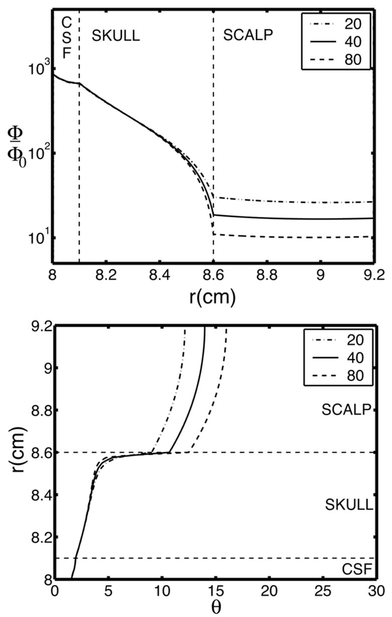
Potential in a 4-sphere model due to a radial dipole source in the inner sphere, that is, the model brain. The three curves in each figure were obtained with the three brain-to-skull conductivity ratios. The model consists of four spherical layers: Sphere radii are (brain, CSF, skull, scalp) = (8.0, 8.1, 8.6, 9.2). Brain and scalp are assumed to have the same conductivity; CSF conductivity is 5 times brain conductivity; 3 brain-to-skull conductivity ratios are plotted (20, 40, 80). (Upper) Fall-off of potential through the thickness of the skull and scalp. Potential is plotted on a logarithmic scale. (b) Angular spread of potential in the skull and scalp. The curves represent the distance at which potential is 50% of its maximum directly above the dipole (θ = 0).

From these simulations we can develop an intuitive picture of current flow in the scalp due to dipole sources in the brain. In brain regions with dense source activity, current flows mainly in the radial direction through the skull into the scalp and spreads outward, while in other regions with less source activity current converges and flows through the skull into the brain. With sources P(r, t) oscillating in time, the current direction reverses every half cycle. There can also be regions that neither inject nor accept scalp current. Thus, different surface regions of the skull behave as skull “sources”, “sinks” or “quiet regions” with respect to the scalp current injection, as a consequence of genuine physiological source activity within the brain. Of course, in genuine heads the picture is more complicated because the conductivity and thickness of the skull and scalp are not uniform. Also, holes or regions of low skull resistance may act as preferential current paths, but the general qualitative idea is valid.

Because of current conservation, scalp current can change while passing a scalp location only by current injection or removal from a skull “source” or “sink” of current directly below the local scalp. In order to determine whether a given scalp location serves as a source or sink for scalp currents, the change in current density (J_s) along the two-dimensional scalp surface may be evaluated. Ohm’s law for linear conductors indicates that current density in the scalp is proportional to the spatial gradient of the potential. The divergence of current density along the scalp is then equivalent to the surface Laplacian ( ${\nabla }_S^2$) of the scalp potential Φ_S:

$${\nabla }_{\mathbf{S}}·{\mathbf{J}}_{\mathbf{S}}=-{\nabla }_{\mathbf{S}}·{\sigma }_S{\nabla }_{\mathbf{S}}{\mathrm{\Phi }}_S=-{\sigma }_S{\nabla }_S^2{\mathrm{\Phi }}_S$$ (3)

where σ_s is the (assumed constant) conductivity of the scalp. Note that the gradient operator ∇_S is the derivative along the scalp surface S, expressed in the two surface coordinates that define the local geometry of the scalp. The surface Laplacian operator $L_S={\nabla }_S^2$ is the second spatial derivative along the two surface coordinates. On a planar surface defined by x and y coordinates:

$$L_S={\nabla }_S^2({\mathrm{\Phi }}_S)=\frac{{\partial }^2{\mathrm{\Phi }}_S}{\partial x^2}+\frac{{\partial }^2{\mathrm{\Phi }}_S}{\partial y^2}$$ (4)

In spherical or ellipsoidal geometries, the expression for the surface Laplacian can be written as derivatives in the corresponding system coordinates. The surface Laplacian can also be calculated for an arbitrary surface geometry, for instance a realistic scalp geometry derived from MRI images (25) by making use of local surface normals (26).

Any change in tangential current flow in the scalp must be due to the emergence of current into the scalp from the skull or the convergence of current into the skull. Thus, the surface Laplacian can be used to detect sources and sinks of current flow into the scalp from the skull. We expect that within the skull, most current flows in the radial direction with minimal flow in tangential directions. Simulations using a spherical model with a poorly conducting skull layer shown in Fig. 4 suggest that this intuition is quite reasonable. Very little smearing of the potential distribution takes place within most of the skull, suggesting minimal tangential skull current. Thus, radial current density in the skull that enters or exits the scalp under an electrode is approximately proportional to the surface Laplacian of the potential at the electrode as formally derived in (5).

Surface Laplacians provide theoretically unique estimates, subject to the usual practical limitations of spatial sampling and noise (5). The surface Laplacian enhances the sensitivity of EEG to sources that are “localized” in superficial cortex within a small distance (2–3 cm in all directions) of the electrode, and reduces the sensitivity of the EEG to deep sources and widespread synchronous superficial sources. Figure 5 summarizes this idea and contrasts the relative sensitivities of scalp potentials and surface Laplacians. Figure 5a demonstrates that the outer surface (scalp) potential due to a radial dipole is always larger than the potential due to a tangential dipole at the same depth in the innermost (brain) sphere of the concentric spheres model. Superficial radial dipole sources make the strongest contributions to scalp potentials. Figure 5b shows a similar simulation for the surface Laplacian. The Laplacian is even more preferentially sensitive to superficial radial dipole sources. Sources at a depth of more than 2 cm (radial or tangential) make negligible contribution to the surface Laplacian. Most tangential sources are likely to occur in fissures and sulci, thus located deeper than radial sources and further reducing their contribution to the surface Laplacian.

Figure 5.

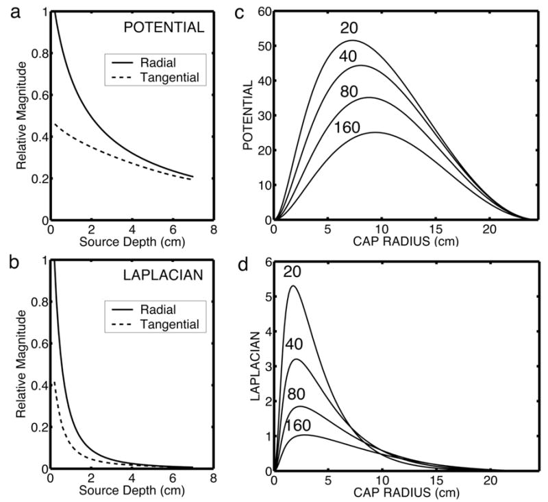
Simulations of sensitivity of potentials and surface Laplacian to dipole sources. Simulations were performed using a 4-sphere model of the head as described in Figure 4. The only parameter varied in these simulations is the brain-to-skull conductivity ratio from 20 to 160. (a) Dependence of potential on source depth for radial and tangential dipoles. Depth is calculated from the top of the brain sphere (r₁ = 8.0). (b) Dependence of surface Laplacian on source depth. (c) Dependence of outer surface (scalp) potential on the spatial extent of dipole layers composed of superficial radial dipole sources at a fixed radial location (r = 7.8). (d) Dependence of the Laplacian on the spatial extent of dipole layers composed of superficial radial dipole sources at a fixed radial location (r = 7.8).

Figures 5c and 5d consider the effect of the spatial extent (expressed as radius of the layer) of dipole layers composed of aligned, synchronous (with no phase difference) superficial radial dipoles at a fixed radius in the brain sphere of the model. Because all sources within each dipole layer are assumed to oscillate in phase (“synchronous” sources), surface potential magnitudes are obtained by simple linear superposition of contributions from small parts of the layers that can be treated as single dipoles. The dipole layers form spherical caps indicated by radii in surface tangential directions. Source strength was fixed by setting the potential across the dipole layer uniformly to 100 μV, roughly matching data obtained with cortical depth recordings. The maximum potential on the scalp sphere, directly above the center of the dipole layer, is shown in Figure 6c for different cap radii. Scalp potential increases with increased layer size up to a dipole layer radius of about 7–8 cm, a diameter of 15 cm spanning about half the distance from occipital to frontal pole on an idealized smooth cortex. By contrast, the surface Laplacian shows the highest response for very small dipole layers of radius of about 2 cm. The large dipole layers (radius larger than about 5 cm) that make a large contribution to the potential make only small contributions to the surface Laplacian.

Figure 6.

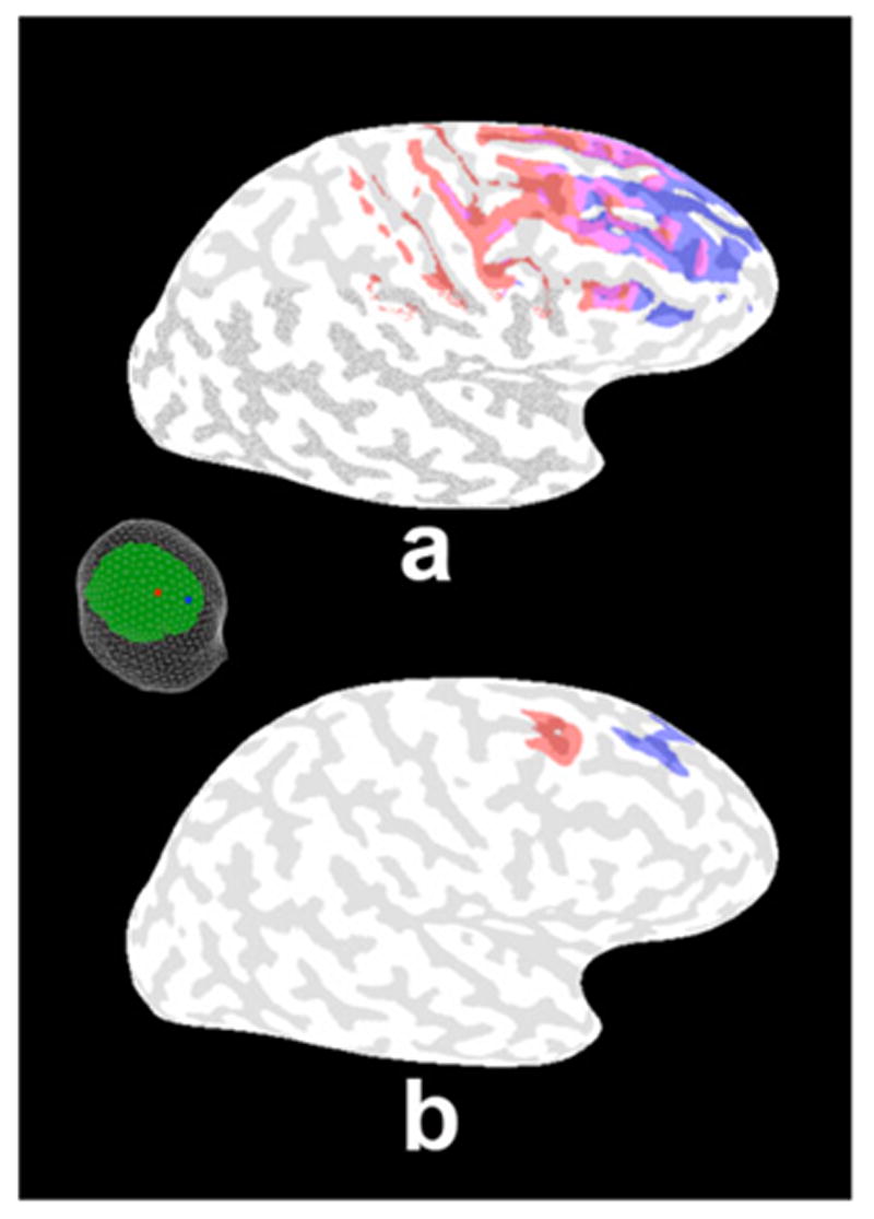
Example half-sensitivity distributions of EEG versus surface Laplacian on the realistic source distribution for two electrodes. The electrode positions are shown in the inset; the electrodes are separated by 5 cm. a. Half-sensitivity distribution of the potentials for each electrode position shown by corresponding color coding (red or blue) on the inflated brain. Regions indicated in purple are contributing significant potentials to both electrodes. b. Sensitivity distribution of the surface Laplacian at the same electrode position. Note that distant sources, more than 2 or 3 cm away from the electrode no longer contribute significantly to the signal at each electrode. Thus, there are two distinct red and blue regions shown on the inflated cortex and no regions of overlap.

The strong influence of source region size on scalp potentials has also been quantified as preferential sensitivity to low spatial frequency components of the source distribution (5,8). The selective sensitivity of the surface Laplacian to smaller source regions is a consequence of its preferential sensitivity to higher spatial frequencies than the scalp potentials, but limited by the separation distances between electrodes and between sources and electrodes (10). In summary, potentials and surface Laplacians are sensitive to different spatial bandwidths of the source distribution. Scalp potentials are a spatially low-pass filtered representation of the source distribution P(r, t), while surface Laplacians are effectively spatially band-pass filtered representations of source distributions. Thus, surface Laplacians serve to complement (but not replace) EEG potentials. Even when localized sources are identified with the surface Laplacian, broadly distributed sources, which make only minimal contributions to the Laplacian, may be making substantial contributions to scalp potentials.

Co-registration of high-resolution EEG with MRI

The sensitivity of the high-resolution EEG obtained with a surface Laplacian is limited to very local sources within a small distance of the electrodes. A Green’s function can be defined for the surface Laplacian by applying the second spatial derivative to the Green’s function for the scalp potential (5, 8, 10). Then a sensitivity distribution can be calculated similar to the potentials and MEG. For convenience we follow the notion of a half-sensitivity volume (23), and define a half-sensitivity distribution as those vertices that contribute at least half the signal contributed by the strongest source position. Figure 6 shows the half-sensitivity distribution for the potential at a pair of electrodes spaced by around 5 cm as shown in the figure inset. The half-sensitivity distributions of the potential at each electrode are indicated by the corresponding colors; they overlap substantially as indicated by the purple regions. The highest sensitivity is at the same location in the cortex as for the potential in Fig. 6a but the surface Laplacian is much less sensitive to distant gyral surfaces.

The dramatic improvement in spatial resolution afforded by high-resolution EEG is demonstrated by comparing these results with the surface Laplacian half-sensitivity distribution in Figure 6b. The surface Laplacians at these two electrodes are sensitive to distinct gyral crowns. The implication is that if the source is localized to the specific gyral surfaces indicated in the figure, the surface Laplacian will isolate the signal corresponding to that source in a single electrode. If the source is not present, or is much larger than the gyral crown, i.e., spanning several gyral surfaces, the surface Laplacian will suppress the signal at the electrode. The implication is that with electrodes spaced by around 2 cm covering the upper surface of the head and the use of a volume conduction model, very detailed measurements of the activity localized to specific gyral surfaces can be accomplished with high-resolution EEG.

Discussion

Spatial filtering versus source localization

The limited evidence available from intracranial recordings in humans does not support the contention that only a few sites in the brain are active in generating most EEG signals (26–28). Although converging evidence from other methods (fMRI or PET) is often provided as support for inverse solutions, or even used to seed these inverse solutions, there may be only minimal theoretical bases to make such connection (30–31). Thus, there remains considerable motivation to approach the problem of locating the generators of the EEG by making improvements to spatial resolution rather than making assumptions about the nature or number of sources. High-resolution EEG methods provide reference-independent estimates of the radial current density in the skull by applying the surface Laplacian operator to the scalp potentials. The radial skull current depends mainly on sources on the local (within 2–3 cm) gyral surfaces directly beneath the electrode. Unlike the inverse problem, which effectively has an infinite number of possible solutions, and requires both a source and a volume conduction model the surface Laplacian approach requires no assumptions about either the sources or the volume conductor, and provides a unique estimate of superficial cortical sources. The only assumption required is a model of the scalp surface which we can approximate by a sphere or an ellipsoid with minimal error (17, 25). The effect of spatial filtering is to focus each electrode on signals that are well-localized; broad source distributions contribute minimally to high-resolution EEG. In practice we have shown that the use of surface Laplacians requires a dense array of electrodes spaced by 3 cm or less (5).

Using a realistic source model we have demonstrated that source localization of high-resolution EEG can be achieved by spatial filtering of the scalp potential distribution. This high-resolution EEG via can be a very effective means of source localization when co-registered with the cortical surface using a volume conduction model. With 2–3 cm electrode spacing on the scalp, adjacent electrodes are apparently sensitive to distinct cortical tissue, allowing for precise localization. The only caveat is that broadly distributed sources will be suppressed by high-resolution EEG; these sources are, in any case, not well-localized, and are better characterized in terms of spatial statistics such as coherence (5).

Can EEG be related to fMRI?

The arguments in this paper suggest that the modeling of EEG signals can benefit substantially from the use of information about source position obtained from MRI and high-resolution EEG algorithms to process the EEG. Although the benefit of accurate geometrical models of the head is severely limited by poor knowledge of the conductivity of the tissues of the head, accurate knowledge of the source positions and the electrode positions can be of considerable utility especially when combined with high-resolution EEG methods. Can we similarly make effective use of fMRI? Although many studies have been published co-registering EEG and fMRI results there appears to be little theoretical basis for making this connection (30). In part this simply reflects the uncertainty in the physiological bases of fMRI and its connection to neuronal activity. But it also reflects the fact that fMRI and EEG are sensitive to very different aspects of brain function that may only partly related even in the same subject and same experiment (5). For instance EEG signals depend strongly on the synchronization of synapses, both within a region producing a dipole source and across cortical regions forming dipole layers on local, regional, or even global scales. We do not know of any relationship between fMRI and the synchrony of cortical sources. Another example is cortical stellate cells that are essentially invisible to EEG and MEG as their spherical shape essentially produces a closed field (30). Due to their high firing rates they potentially make an important contribution to the fMRI signal while making no external electric or magnetic field. Despite the obvious appeal of combining the high temporal resolution with the high spatial resolution of fMRI, the only obvious connection between these measures is the subject and the experiment. EEG and fMRI are selectively sensitive to different types of brain activity that may overlap spatially only in very limited instances (30).

Conclusions

In summary, we have demonstrated that by applying spatial filters to EEG recordings, we can obtain a high-resolution EEG that can be co-registered to source models based on anatomical MRI. This combination of filtering and source modeling allows us to localize the signals at high-resolution EEG electrodes to specific gyral surfaces. Conventional EEG and MEG using a single magnetometer coil have far poorer spatial resolution and are not easily localized using a head model although further improvements to MEG can be anticipated with the use of planar gradiometer coils. Source position information from MRI is a considerable aid to determining the sources of high-resolution EEG signals. In contrast, information about tissue boundaries, especially skull and scalp, cannot be effectively used because of the lack of information about conductivities of the tissues. Developments in MRI technology to directly estimate tissue conductivity may in the future be used to improve models of the head (32). At the present time, the main utility of EEG in clinical pathologies such as tumors and stroke is to assess dynamic changes in brain function (2, 3, 33).

References

- 1.Walter WG. Traps, tricks and triumphs in EEG: 1936–1966. Electroencephalogr Clin Neurophysiol. 1967;22(4):393. [PubMed] [Google Scholar]
- 2.Nagata K, Tagawa K, Hiroi S, Shishido F, Uemera K. Topographic electroencephalographic study of cerebral infarction using computed mapping of EEG. Journal of Cerebral Blood Flow and Metabolism. 1982;2:79–88. doi: 10.1038/jcbfm.1982.9. [DOI] [PubMed] [Google Scholar]
- 3.Nuwer MR, Jordan SE. Ahn SS Evaluation of stroke using EEG frequency analysis and topographic mapping. Neurology. 1987;37:1153–9. doi: 10.1212/wnl.37.7.1153. [DOI] [PubMed] [Google Scholar]
- 4.Nunez PL. Toward a quantitative description of large scale neocortical dynamic function and EEG. Behavioral and Brain Sciences. 2000;23:371–398. doi: 10.1017/s0140525x00003253. [DOI] [PubMed] [Google Scholar]
- 5.Nunez PL, Srinivasan R. Electric Fields of the Brain: The Neurophysics of EEG. 2. Oxford UP; New York: 2006. [Google Scholar]
- 6.Braitenberg V, Schuz A. Anatomy of the Cortex: Statistics and Geometry. New York: Springer-Verlag; 1991. [Google Scholar]
- 7.Nunez PL. Electric Fields of the Brain: The Neurophysics of EEG. Oxford UP: New York; 1981. [Google Scholar]
- 8.Srinivasan R, Nunez PL, Silberstein RB. Spatial filtering and neocortical dynamics: estimates of EEG coherence. IEEE Transactions on Biomedical Engineering. 1998;45:814–825. doi: 10.1109/10.686789. [DOI] [PubMed] [Google Scholar]
- 9.Nunez PL, Silberstein RB, Cadusch PJ, Wijesinghe R, Westdorp AF, Srinivasan R. A theoretical and experimental study of high resolution EEG based on surface Laplacians and cortical imaging. Electroencephalography and Clinical Neurophysiology. 1994;90:40–57. doi: 10.1016/0013-4694(94)90112-0. [DOI] [PubMed] [Google Scholar]
- 10.Srinivasan R, Nunez PL, Tucker DM, Silberstein RB, Cadusch PJ. Spatial sampling and filtering of EEG with spline-Laplacians to estimate cortical potentials. Brain Topography. 1996;8:355–366. doi: 10.1007/BF01186911. [DOI] [PubMed] [Google Scholar]
- 11.Nunez PL, Srinivasan R, Westdorp AF, Wijesinghe RS, Tucker DM, Silberstein RB, Cadusch PJ. EEG coherency I: Statistics, reference electrode, volume conduction, Laplacians, cortical imaging, and interpretation at multiple scales. Electroencephalography and Clinical Neurophysiology. 1997;103:516–527. doi: 10.1016/s0013-4694(97)00066-7. [DOI] [PubMed] [Google Scholar]
- 12.Nunez PL, Silberstein RB, Shi Z, Carpenter MR, Srinivasan R, Tucker DM, Doran SM, Cadusch PJ, Wijesinghe RS. EEG coherence II: Experimental measures of multiple coherence measures. Electroencephalography and Clinical Neurophysiology. 1999;110:469–486. doi: 10.1016/s1388-2457(98)00043-1. [DOI] [PubMed] [Google Scholar]
- 13.Lopes da Silva F. Functional localization using EEG and/or MEG data: volume conductor and source models. Magnetic Resonance Imaging. 2004;22:1533–38. doi: 10.1016/j.mri.2004.10.010. [DOI] [PubMed] [Google Scholar]
- 14.Cohen D, Cuffin BN, Yunokuchi K, Maniewski R, Purcell C, Cosgrove GR, Ives J, Kennedy JG, Schomer DL. MEG versus EEG localization test using implanted sources in the human brain. Ann Neurol. 1990;28(6):811–7. doi: 10.1002/ana.410280613. [DOI] [PubMed] [Google Scholar]
- 15.Nunez PL. A method to estimate local skull resistance in living subjects. IEEE Transactions on Biomedical Engineering. 1987;34:902–904. doi: 10.1109/tbme.1987.326104. [DOI] [PubMed] [Google Scholar]
- 16.Poulnot M, Lesser G, Law SK, Westdorp AF, Nunez PL. Brain Physics Group, Tulane University; New Orleans: 1989. Unpublished study. [Google Scholar]
- 17.Law S. Thickness and resistivity variations over the upper surface of human skull. Brain Topography. 1993;3:99–109. doi: 10.1007/BF01191074. [DOI] [PubMed] [Google Scholar]
- 18.Yan Y, Nunez PL, Hart RT. Finite element model of the human head: scalp potentials due to dipole sources. Medical and Biological Engineering and Computing. 1991;29:475–481. doi: 10.1007/BF02442317. [DOI] [PubMed] [Google Scholar]
- 19.Oostendorp T, Delbeke J, Stegeman DF. The conductivity of human skull: results of in vivo and in vitro measurements. IEEE Transactions on Biomedical Engineering. 2000;47:1487–1492. doi: 10.1109/TBME.2000.880100. [DOI] [PubMed] [Google Scholar]
- 20.Akhtari M, Bryant HC, Mamelak AN, Heller L, Shih JJ, Mandelkern M, Matlachov A, Ranken DM, Best ED, Sutherling WW. Conductivities of three-layer human skull. Brain Topography. 2000;13:29–42. doi: 10.1023/a:1007882102297. [DOI] [PubMed] [Google Scholar]
- 21.Hoekema R, Wieneke GH, Leijten FSS, van Veelen CWM, van Rijen PC, Huiskamp GJM, Ansems J, van Huffelen AC. Measurement of the conductivity of skull temporarily removed during epilepsy surgery. Brain Topography. 2003;16:29–38. doi: 10.1023/a:1025606415858. [DOI] [PubMed] [Google Scholar]
- 22.Hamaleinen M, Hari R, Ilmoniemi RJ, Knuutila J, Lounasmaa OV. Magnetoencephalography-theory, instrumentation, and applications to noninvasive studies of the working human brain. Reviews of Modern Physics 65. 1993;413:497. [Google Scholar]
- 23.Malmivuo J, Plonsey R. Bioelectromagnetism. Oxford UP: New York; 1995. [Google Scholar]
- 24.Srinivasan R, Russell DP, Edelman GM, Tononi G. Increased synchronization of neuromagnetic responses during conscious perception. Journal of Neuroscience. 1999;19:5345–5348. doi: 10.1523/JNEUROSCI.19-13-05435.1999. [DOI] [PMC free article] [PubMed] [Google Scholar]
- 25.Babiloni F, Babiloni C, Carducci F, Fattorini L, Onaratti P, Urbano A. Spline Laplacian estimate of EEG potentials over a realistic magnetic resonance-constructed scalp surface model. Electroencephalography and Clinical Neurophysiology. 1996;98:204–215. doi: 10.1016/0013-4694(96)00284-2. [DOI] [PubMed] [Google Scholar]
- 26.Srinivasan R. Methods to improve the spatial resolution of EEG. International Journal of Bioelectromagnetism. 1999;1:102–111. [Google Scholar]
- 27.Aoki F, Fetz EE, Shupe L, Lettich E, Ojemann GA. Changes in power and coherence of brain activity in human sensorimotor cortex during performance of visuomotor tasks. Biosystems. 2001;63:89–99. doi: 10.1016/s0303-2647(01)00149-6. [DOI] [PubMed] [Google Scholar]
- 28.Raghavachari S, Kahana MJ, Rizzuto DS, Caplan JB, Kirschen MP, Bourgeois B, Madsen JR, Lisman JE. Gating of human theta oscillations by a working memory task. Journal of Neuroscience. 2001;21:3175–3180. doi: 10.1523/JNEUROSCI.21-09-03175.2001. [DOI] [PMC free article] [PubMed] [Google Scholar]
- 29.Menon V, Freeman WJ, Cutillo BA, Desmond JE, Ward MF, Bressler SL, Laxer KD, Barbaro N, Gevins AS. Spatio-temporal correlations in human gamma band electrocorticograms. Electroencephalography and Clinical Neurophysiology. 1996;98:89–102. doi: 10.1016/0013-4694(95)00206-5. [DOI] [PubMed] [Google Scholar]
- 30.Nunez PL, Silberstein RB. On the relationship of synaptic activity to macroscopic measurements: Does co-registration of EEG with fMRI make sense? Brain Topography. 2000;13:79–96. doi: 10.1023/a:1026683200895. [DOI] [PubMed] [Google Scholar]
- 31.Horowitz B, Poeppel D. How can EEG/MEG and fMRI/PET be combined? Human Brain Mapping. 2002;17:1–3. doi: 10.1002/hbm.10057. [DOI] [PMC free article] [PubMed] [Google Scholar]
- 32.Ueno S, Iriguchi N. Impedance magnetic resonance imaging: A method for imaging impedance distributions based on magnetic resonance imaging. Journal of Applied Physics. 1998;83:6450–6452. [Google Scholar]
- 33.Luu P, Tucker DM, Englandr R, Lockfield A, Lutsep H, Oken B. Localizing acute stroke-related EEG changes: assessing the effects of spatial undersampling. 2001;18:302–317. doi: 10.1097/00004691-200107000-00002. [DOI] [PubMed] [Google Scholar]