

Abstract
We investigated spatial properties of the source distributions that generate scalp electroencephalographic (EEG) oscillations. The inherent complexity of the spatiotemporal dynamics of EEG oscillations indicates that conceptual models that view source activity as consisting of only of a few “equivalent dipoles” are inadequate. We present an approach that uses volume conduction models to characterize the distinct spatial filtering of cortical source activity by average-reference EEG, high-resolution EEG, and magnetoencephalography (MEG). By comparing these three measures, we can make inferences about the sources of EEG oscillations without having to make prior assumptions about the sources. We apply this approach to spontaneous EEG oscillations observed with eyes closed at rest. Both EEG and MEG recordings show robust alpha rhythms over posterior regions of the cortex; however, the dominant frequency of these rhythms varies between EEG and MEG recordings. Frontal alpha and theta rhythms are generated almost exclusively by superficial radial dipole layers that generate robust EEG signals but very little MEG signals; these sources are presumably mainly in the gyral crowns of frontal cortex. MEG and high-resolution EEG estimates of alpha rhythms provide evidence of local tangential and radial sources in the posterior cortex, lying mainly on sulcal and gyral surfaces. Despite the detailed information about local radial and tangential sources potentially afforded by high-resolution EEG and MEG, it is also evident that the alpha and theta rhythms receive contributions from non-local source activity, for instance large dipole layers distributed over lobeal or (potentially) even larger spatial scales.
Keywords: high-resolution, electroencephalography (EEG), magnetoencephalography (MEG), source localization, alpha rhythms, theta rhythms
Spatial properties of EEG oscillations
Electroencephalograhy (EEG) is a very large-scale measure of brain source activity, apparently recording synaptic activity synchronized over macroscopic (centimeter), regional, and even whole brain spatial scales (Nunez 2000; Nunez and Srinivasan, 2006). Synchrony among neural populations in compact regions of the brain produces localized dipole current sources. Synchrony among neural populations distributed across the cortex can give rise to regional or global networks consisting of many dipole sources. EEG oscillations reflect brain source activity that has been selectively filtered (spatially) by the volume conduction of currents through the head. In this chapter, we investigate spatial properties of the sources underlying EEG oscillations using volume conduction models, high-resolution EEG methods, and simultaneous recordings of the brain’s magnetic field or magnetoencephalography (MEG).
Spectral analysis methods have facilitated quantifying EEG dynamics in terms of the dominant frequencies, power (or amplitude), phase, and coherence. Normal waking alpha rhythms (8–12 Hz) usually have larger amplitudes over posterior regions, but are typically recorded over widespread scalp regions and may be desynchronized (substantially reduced in amplitude) by eye opening, drowsiness and by moderate to difficult mental tasks. The EEG literature sometimes treats alpha primarily as an occipital-parietal rhythm; smaller amplitude alpha rhythms recorded in frontal or prefrontal electrodes are often assumed to be volume conducted currents generated by sources confined to posterior regions of the cortex. Yet in the classical studies by Jasper and Penfield (1949), alpha rhythms were recorded from nearly the entire upper cortical surface (including frontal and prefrontal areas) in a large population of patients awake prior to surgery. Scalp EEG coherence studies using high-resolution EEG methods have demonstrated unequivocally that the alpha rhythm exhibits spatial structure with robust long and short range correlations that change with age and brain state (Nunez 1995; Srinivasan, 1999; Nunez et al., 2001). Such coherence changes often include frontal and prefrontal regions. Furthermore, the term “alpha rhythm” appears to encompass several oscillations having different sensitivities to cognitive or motor tasks (Andrew and Pfurtscheller, 1996, 1997; Klimesch et al 1999; Petsche and Etlinger 1998; Pfurtscheller and Neuper 1992; Pfurtscheller and Lopes da Silva 1999). In high-resolution EEG studies, the upper and lower alpha bands are modulated in opposite directions in a working memory task (Nunez et al., 2001). Oscillations in other frequency bands, e.g., theta (4–7 Hz) and gamma bands (30–70 Hz) also exhibit complex patterns of power and coherence that are modulated by cognitive processes such as working memory (Nunez et al., 2001; Schack et al., 2002) and perceptual binding (Rose et al., 2005).
The inherent complexity of the spatiotemporal dynamics of EEG oscillations indicates that conceptual models which always associate EEG signals with a focal generator are inadequate. The EEG inverse problem has no unique solution and all published solution methods require additional assumptions. For instance, a common approach is to fit a small (often only one) dipole source position, orientation, and strength from the scalp potentials. In some cases, such as short latency sensory evoked potentials or epileptic discharges, the assumption that a single focal region of the cortex is the main EEG generator may justify modeling signals with a single dipole source. However, in general, EEG oscillations can evidently be generated regionally or even globally, involving neural populations acting in concert (Nunez and Srinivasan, 2006). The existence of localized generators is apparently not a general property of EEG data. EEG signals related to cognitive processes probably involve distributed cortical tissue, perhaps in multiple, widely separated brain regions. In this case the results of dipole localization can only be interpreted as “equivalent dipoles” which are just descriptors of the potential distribution. The objective of any realistic source analysis is to characterize sources without making prior assumptions about the actual nature of the sources.
Source models for EEG oscillations
The dipole approximation to cortical current sources provides the basis for any realistic EEG source model. It is based on the idea that at large distances, any complex current distribution in a small region of the cortex can be approximated by a “dipole” or more accurately, a dipole moment per unit volume. A “large distance” in this case is at least 3 or 4 times the distance between the effective poles of the dipole. Superficial gyral surfaces are located at roughly 1.5 cm from scalp electrodes. In this context, the dipole approximation appears valid only for superficial cortical tissue with a maximum extent in any dimension of roughly 0.5 cm or less. Macrocolumns (approximately 3 mm diameter) provide a convenient scale to picture dipoles. There can be multiple active dipole sources within a 2 cm2 gyral crown; that is, the crown forms a small dipole layer. The sources of many (if not most) EEG phenomena may then be pictured as thousands cortical dipoles, mainly oriented perpendicular to the cortical surface forming dipole layers (or folded dipole sheets. However, we emphasize that the word “dipole” is actually just convenient jargon for the continuously varying dipole moment per unit volume or meso-sources P(r, t), as described in Nunez and Srinivasan (2006).
If we assume that EEG sources consist of thousands of dipoles oriented perpendicular to the cortical surface, “localized” sources can be defined approximately as dipole layers of non-zero spatial extent that are relatively segregated from the surrounding areas of cortex. In the context of EEG dynamics, segregation of a dipole layer implies that the time-dependencies of dipole source strengths in the layer are temporally correlated to each other and uncorrelated (or at least much more weakly correlated) to other dipoles in the surrounding cortex. In general, we expect that EEG signals are generated by multiple contributions from many dipole layers of different sizes and locations, perhaps even overlapping in location. For instance, EEG signals may be generated in one region of the brain by a combination of strong dipole sources at small spatial scales (say a dipole layer of about 1 cm diameter) in one frequency band and moderately correlated dipole layers, forming a weaker sources at larger spatial scales (say 5–10 cm), and producing oscillations in either a distinct or overlapping frequency band.
Spatial filtering of scalp potentials
The relationship between scalp potentials Φ(r, t) and the intermediate scale meso-source function P(r, t) or dipole moment per unit volume (μA/mm2) can be written in terms of a Green’s function GE (r, r′) that describes the head volume conductor:
| (1) |
The Green’s function expresses the relationship between a unit source at location r′ and the measurement point on the scalp surface r; it depends only on the properties of volume conduction in the head. The potential anywhere in the brain or scalp surface is then expressed as an integral (or weighted sum) of contributions from all meso-sources in brain. The weight given to each source depends on the locations and conductivities of the different tissues in the head. For convenience of this discussion, the brain volume may be parceled into N tissue masses or voxels of volume ΔV, each producing its own time-dependent meso-source strength pn(t) ≅ P(r, t) ΔV(r). Scalp potential at any location r, given by Eq (1), may be expressed as the simple weighted sum
| (2) |
The weighting coefficients gn are a discrete version of the Green’s function and depend on the properties of the volume conductor and the locations of each source and the measurement location r; they are essentially the inverse electrical distances between sources and surface locations. The sum has 3N terms reflecting because each voxel n produces a meso-source vector pn(t).
Many properties of EEG recordings of neural oscillations can be inferred by studying the properties of head volume conduction independent of any specific source configuration or experimental data. The so-called “4-sphere model”, consisting of an inner brain sphere surrounded by concentric spherical shells has proven to be very a useful model of head volume conduction in these studies. The essential feature of such models is low skull conductivity compared to brain, CSF, skull, or scalp tissue. This model has been used extensively in simulation studies of surface Laplacians (Nunez et al., 1994; Srinivasan et al., 1996), EEG coherence estimates (Nunez et al., 1997, 1999; Srinivasan et al., 1998) and forms the basis for a number of approaches to source localization (Lopes da Silva 2004). The thickness and conductivity ratios of the spherical shells are the essential features of the model. We investigated the 4-sphere model for brain-to-skull conductivity ratios (σ1/σ3 = 20–80) spanning the range of most published estimates (reviewed in Nunez and Srinivasan, 2006). As found in previous simulation studies, the results depend mainly on the qualitative property of poor skull conductivity in this range. The large uncertainty in estimates of skull conductivity in any head model whether concentric or realistic, is far more important than the errors introduced by approximating the geometry of the head, which have been estimated at 10–15 % in simulation studies that compare spherical models to realistic Finite Element models (Yan et al. 1991).
Source analysis by high-resolution EEG methods
High-resolution EEG methods are based on a conceptual framework that differs substantially from that of source localization. The current source distribution in the cranial volume cannot be estimated uniquely using only data recorded on the scalp surface. Assumptions must be applied by all source localization methods in order to arrive at source location estimates. By contrast, high-resolution EEG methods do not require any assumptions about the sources; instead they enhance the sensitivity of each electrode. The EEG signal recorded at each electrode is a spatial average of active current sources distributed over a volume of brain space. The size and shape of this volume depends on a number of factors including the volume conduction properties of the head and choice of reference electrode. The contribution of each source to this spatial average depends on the electrical distance between source and electrode, source orientation and source strength as represented in Eq (2). When two electrodes are very closely spaced, similar signals are recorded because they record the average activity in largely overlapping volumes of tissue. High-resolution EEG methods, such as the surface Laplacian, have the effect of reducing the effective volume that each electrode averages, thereby improving spatial resolution. As discussed in Nunez and Srinivasan (2006), the surface Laplacian emphasizes certain types of source activity—mainly superficial, localized sources (as defined above). At the same time, the Laplacian deemphasizes other kinds of activity--deep sources and widespread coherent superficial sources.
Surface Laplacians provide theoretically unique estimates of dura potential, subject to the usual practical limitations of spatial sampling and noise. Both simulations and application to experimental EEG data have shown that surface Laplacians are highly consistent with estimates of dura potential (dura imaging) obtained with 3 or 4-sphere volume conduction head models (Nunez et al., 1994; Nunez et al., 2001). The surface Laplacian enhances the sensitivity of EEG to sources that are “localized” in superficial cortex within a small distance (2–3 cm in all directions) of the electrode, and reduces the sensitivity of the EEG to deep sources and widespread synchronous superficial sources. Figure 1 summarizes this idea and contrasts the relative sensitivities of scalp potentials and surface Laplacians. Figure 1a demonstrates that the outer surface (scalp) potential due to a radial dipole is always larger than the potential due to a tangential dipole at the same depth in the innermost (brain) sphere of the concentric spheres model. Superficial radial dipole sources make the strongest contributions to scalp potentials. Figure 1b shows a similar simulation for the surface Laplacian. The Laplacian is even more preferentially sensitive to superficial radial dipole sources. Sources at a depth of more than 2 cm (radial or tangential) make negligible contribution to the surface Laplacian. Most tangential sources are likely to occur in fissures and sulci, thus located deeper than radial sources and further reducing their contribution to the surface Laplacian.
Fig. 1.
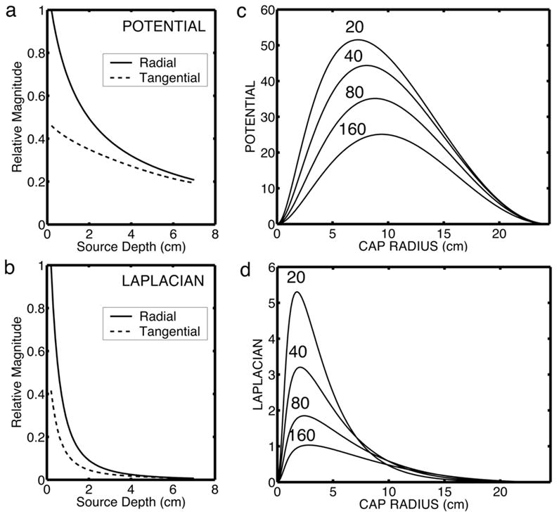
Simulations of sensitivity of potentials and surface Laplacian to dipole sources. Simulations were performed using a “4-sphere” model of the head. The spherical surfaces are (1) brain, (2) cerebrospinal fluid (CSF), (3) skull, and (4) scalp. Potentials and Laplacians are calculated on the outer (scalp) surface. Our standard model parameters are the radii of the spheres (r1 = 8.0 cm, r2 = 8.1 cm, r3 = 8.6 cm, r4 = 9.2 cm) and the conductivity ratios between the spherical shell regions (σ12 = 0.2, σ13 = 40, σ14 = 1). The only parameter varied in these simulations is the brain-to-skull conductivity ratio (σ13) from 20 to 160. (a) Dependence of potential on source depth for radial and tangential dipoles. Depth is calculated from the top of the brain sphere (r1 = 8.0). (b) Dependence of surface Laplacian on source depth. (c) Dependence of outer surface (scalp) potential on the spatial extent of dipole layers composed of superficial radial dipole sources at a fixed radial location (r = 7.8). (d) Dependence of the Laplacian on the spatial extent of dipole layers composed of superficial radial dipole sources at a fixed radial location (r = 7.8).
Figures 1c and 1d demonstrate the effect of the spatial extent (expressed as radius of the layer) of dipole layers composed of aligned, synchronous (with no phase difference) superficial radial dipoles at a fixed radius in the brain sphere of the model. Because all sources within each dipole layer are assumed to oscillate in phase (“synchronous” sources), surface potential magnitudes are obtained by simple linear superposition of contributions from small parts of the layers that can be treated as single dipoles. The dipole layers form spherical caps indicated by radii in surface tangential directions. Source strength was fixed by setting the potential across the dipole layer uniformly to 100 μV, roughly matching data obtained with cortical depth recordings (see review in Nunez 1995). The maximum potential on the scalp sphere, directly above the center of the dipole layer, is shown in Figure 1c for different cap radii. Scalp potential increases with increased layer size up to a dipole layer radius of about 7–8 cm, a diameter of 15 cm spanning about half the distance from occipital to frontal pole on an idealized smooth cortex. By contrast, the surface Laplacian shows the highest response for very small dipole layers of radius of about 2 cm. The large dipole layers (radius larger than about 5 cm) that make a large contribution to the potential make only small contributions to the surface Laplacian.
The strong influence of source region size on scalp potentials has also been quantified as preferential sensitivity to low spatial frequency components of the source distribution (Srinivasan et al., 1998; Nunez and Srinivasan, 2006). The selective sensitivity of the surface Laplacian to smaller source regions is a consequence of its preferential sensitivity to higher spatial frequencies than the scalp potentials, but limited by the separation distances between electrodes and between sources and electrodes (Srinivasan et al., 1996). In summary, potentials and surface Laplacians are sensitive to different spatial bandwidths of the source distribution. Scalp potentials are a spatially low-pass filtered representation of the meso-source distribution P(r, t), while surface Laplacians are effectively spatially band-pass filtered representations of source distributions. Thus, surface Laplacians serve to complement (but not replace) EEG potentials. Even when localized sources are identified with the surface Laplacian, broadly distributed sources, which make only minimal contributions to the Laplacian, may be making substantial contributions to scalp potentials.
Magnetoencephalography
MEG (magnetoencephalography) is a relatively new technology that provides useful insights into sources when used as an adjunct to EEG measurements. One common but entirely erroneous idea is that MEG spatial resolution is superior to EEG spatial resolution, and that MEG should simply replace EEG in order to extract more accurate information about sources. A much more accurate view is that MEG and EEG are selectively sensitive to different sources; this can be either an advantage or disadvantage to MEG, depending on application. The external magnetic field generated by a radial dipole in a spherically symmetric volume conductor (layered or homogeneous) is zero (Nunez, 1986). Thus, MEG recordings using magnetometer coils tend to filter out signals from dipole sources with axes oriented perpendicular to the scalp surface. These meso-sources lay mostly along the gyral surfaces in the cortex. That is, gyral dipole sources tend to be more nearly perpendicular to the scalp surface than sources in fissures and sulci, although such cortical surface symmetry is not fully satisfied in genuine brains. Given the irregularity of cortical surfaces, gyri sources can easily have non-negligible dipole moments in tangential directions. But for the most part, MEG appears to be more sensitive to tangential dipole sources which lie principally on sulcal walls and less sensitive to sources along gyral surfaces.
By contrast, the maximum outer surface potential due to a superficial radial dipole (cortical) in a four concentric spheres model (brain, CSF, skull, and scalp) is about two to three times the maximum surface potential of a tangential dipole at the same strength and depth, as shown in Figure 1. Thus, we expect EEG to be more sensitive to sources in cortical gyri as indicated and less sensitive to sources in cortical sulci. MEG and EEG are preferentially sensitive to different cortical sources. The sensitivity of high-resolution EEG estimates is even more selective for superficial radial dipoles forming small dipole layers, emphasizing the distinction from MEG sources. This suggests that the addition of simultaneous MEG recordings may refine the inferences about sources obtained with EEG recordings.
A concrete example of differences between MEG, unprocessed EEG and high-resolution EEG estimates obtained from the surface Laplacian are presented in the simulations of Fig. 2. The locations of three radial dipoles are indicated by open (negative pole up) and closed (positive pole up) circles. The ± signs indicate the two poles of a single tangential dipole. Simulated EEG, cortical potential (potential on the surface of the brain sphere), and scalp surface Laplacian were calculated using the 4-sphere head model. The two rows of plots show the same 4-source configuration. In row A, the four dipoles have equal strength (dipole moments); in row B the tangential dipole has a dipole moment that is five time larger than the radial dipoles. In each row, the plotted spatial distribution of the magnetic field is due only to the single tangential dipole (since all radial dipoles make zero contribution in the spherical head model), but with magnitude five times larger in case B. In case A, scalp potential is dominated by the radial dipoles. The surface Laplacian accurately locates the three radial sources and closely mimics the cortical potential. In case B, the scalp potential plot reveals the strong influence of the stronger tangential dipole and a generally more complex potential distribution. For instance, the potential directly over the radial source at the upper left is zero, due to cancellation by the stronger tangential dipole potential. In both rows, the Laplacian is effective in locating the three radial sources and closely approximates the cortical potential.
Fig. 2.
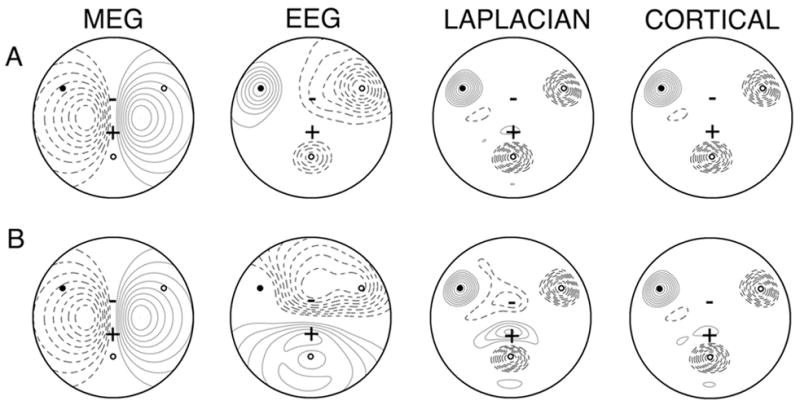
Example spatial distributions of magnetic field (simulated MEG) and potential (simulated EEG) generated by four dipole sources. Three radial dipoles are indicated by open (negative pole up) and filled (positive pole up) circles. The ± signs indicate the two poles of a single tangential dipole. Radial dipoles are located 0.2 cm below the brain surface in the spherical model. The tangential dipole is located 0.8 cm below the brain surface. The MEG field is plotted on a sphere 2.8 cm above the scalp surface. The EEG, cortical potential and surface Laplacian were calculated using the four concentric spheres model of Fig. 2–6 (brain to skull conductivity equal to 40). Each map was normalized with respect to its maximum value to emphasize relative magnitudes. Iso-contours are plotted in steps of 10% of the maximum value. Positive field values are indicated by solid contour lines and negative fields indicated by dashed contours. (Row A) All four dipoles have identical dipole moments. (Row B) The strength of the tangential dipole is five times the strength of the three radial dipoles.
The examples in Fig. 2 illustrate that arguments about the relative accuracies of MEG, EEG and high-resolution EEG must depend critically on the nature of the sources. This general idea has also been confirmed experimentally in animal models using depth recordings, cortical surface recordings and extra-cranial MEG and EEG (Okada et al. 1999). Figure 2A shows that spatial distributions of potential and Laplacian indicate the positions of the three radial sources; MEG provides information that is entirely distinct from the EEG. By contrast, Fig. 2B (stronger tangential dipole) shows substantial similarities between EEG and MEG. Both measures provide good evidence for the stronger tangential source, while the surface Laplacian provides additional information about superficial radial dipoles that is not apparent in either the MEG or unprocessed EEG. The combination of MEG to detect deeper tangential dipoles and high-resolution EEG to detect superficial radial dipoles yields an accurate picture of the source distribution in both examples.
The source distributions underlying the EEG and MEG are generally complex and distributed over the cortex, quite unlike the simple examples of Fig. 2. The sources are plausibly pictured as dipole layers composed of synchronous dipoles oriented perpendicular to the local cortical surface (Nunez 1995; Nunez and Srinivasan 2006). EEG is preferentially sensitive to large radial dipole layers, consisting of many gyral surfaces; whereas synchronous sources in the intervening sulcal folds tend to cancel. High-resolution EEG methods focus the sensitivity of EEG electrodes on superficial dipole layers located close (within 2–3 cm) to the electrode. By contrast, MEG is relatively insensitive to these large source distributions that appear to dominate most EEG recordings. Rather, MEG tends to detect only sources at edges of dipole layers that extend into one sulcal wall since the dipoles on opposite sides of sulci tend to produce canceling magnetic fields.
Simultaneous EEG and MEG recording
We describe here a preliminary study of spontaneous EEG sources; conventional average-reference EEG, high-resolution EEG estimates (obtained with the New Orleans spline-Laplacian algorithm, Nunez and Srinivasan, 2006), and simultaneous MEG recordings are compared to obtain inferences about the underlying sources. The approach described here can be extended to event-related dynamics, evoked potentials, or any other scalp recorded EEG signals.
Spontaneous EEG exhibited by 2 of 6 subjects who participated in the experiment is presented. These two subjects were selected because their data captured the essential issues for comparisons between EEG, Laplacians, and MEG. Informed consent was obtained for each subject. The data were collected using 127 EEG channels (ANT, Netherlands) and 148 MEG channels (4D Neuroimaging, San Diego, USA) at Scripps Hospital in La Jolla, California. Figure 3 shows the positions of the two recording arrays. While EEG electrodes are located on the scalp, MEG sensors are some distance (~ 2 cm) above the head. To facilitate our comparisons of the three measures we have organized the electrodes into regional groups and present our results in terms of these regional groups of electrodes and sensors.
Fig. 3.
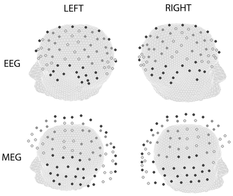
EEG electrode and MEG sensor positions used in the study: 127 EEG electrodes and 148 MEG sensors (magnetometers). The EEG electrodes are located on the scalp, whereas the MEG sensors are located around 2 cm from the scalp in a helmet (not shown). The EEG electrodes were organized into regional groups based on the nearest 10/20 electrode position. The MEG sensors were similarly grouped by first projecting sensor positions onto the head. The labels in each figure indicate the groups: LO – left occipital, RO- right occipital, LT – left temporal, RT – right temporal, LP – left parietal, RP – right parietal, LM – left motor, RM – right motor, LF – left frontal, RF – right frontal, LPF – left prefrontal, RPF – right prefrontal, and MID –midline. Two views of the head are presented to show left and right hemisphere electrodes. The upper row shows the EEG electrode locations and the lower plots show the MEG electrode locations. In each plot, midline (MID) and temporal (LT and RT) electrodes and sensors are indicated in black. Occipital (LO and RO), motor (LM and RM) and prefrontal (LPF and RPF) electrodes and sensors are indicated by light gray circles with a black border. Frontal (LF and RF) and parietal (LP and RP) electrodes and sensors are indicated by dark gray circles.
The EEG amplifier was powered with a battery and placed inside the shielded room, and fiber-optic cables were used to transmit the EEG signals to the acquisition computer outside the room. Since the EEG and MEG signals were sampled simultaneously but by independent amplifiers and A/D cards, we introduced a random trigger signal into both amplifiers in order to synchronize the recordings. The EEG signals were sampled at 931 Hz, and MEG signals were sampled at 1018 Hz. The EEG data was referenced to the instantaneous average potential (“average reference potential”). Each subject was asked to rest with eyes closed for four minutes, followed by four minutes at rest with eyes open.
Estimated equipment and room noise were removed from the raw MEG data by digital filtering, using reference coils positioned in the dewar above the array of MEG coils (Srinivasan et al., 1999). Both EEG and MEG data were Fourier transformed using two second epochs corresponding to a frequency resolution Δf = 0.5 Hz. We focused on the dominant theta and alpha band peaks in the observed spectra in order to avoid most artifact such as eye movement (or eye blinks) and muscle artifact (EMG).
Spectra of average-reference EEG, high-resolution EEG, and MEG
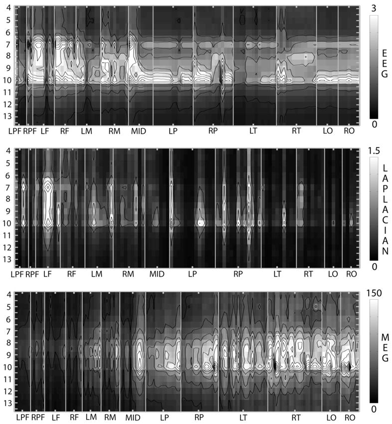
Figure 4 shows rms amplitude spectra at all electrodes or MEG sensors for one subject (SL) at rest with eyes closed. The upper plot shows the average-reference EEG amplitude spectra; the middle plot shows the Laplacian spectra; the lower plot shows the MEG amplitude spectra. Since these measures have units we focused on frequencies with clear peaks in the spectrum of each channel. This subject shows a robust alpha rhythm with all three experimental measures.
Figure 4.
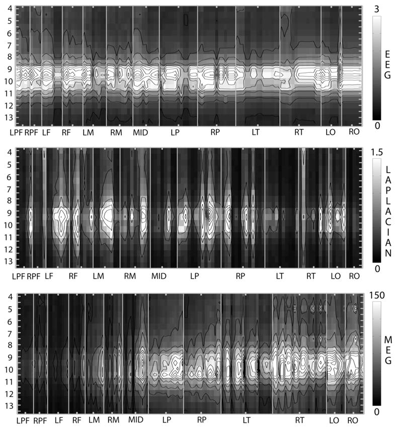
RMS amplitude spectra for subject SL, a 24 year old female. Power spectra were obtained with 0.5 Hz resolution from 4 minutes of eyes closed resting EEG and MEG. Spectra are shown over the band 4 to 13.5 Hz as indicated by the vertical axes. MEG and EEG channels have been sorted into regional groups as indicated by horizontal axes labels, as shown in Figure 3. Upper: Rms amplitude spectra of average reference EEG in units of . Grayscale values are indicated by the color bar. Contours are drawn at intervals of . Middle: Rms amplitude spectra of Laplacian in units of . Grayscale values are indicated by the color bar. Contours are drawn at intervals of 0.25 . Lower: Rms amplitude spectra of MEG in units of (femtoTesla per root Hz). Grayscale values are indicated by the color bar. Contours are drawn at intervals of .
In the average-reference EEG (upper), almost all channels show a peak amplitude at 9.5 Hz. At this peak, the alpha rhythm appears to be widespread over the upper brain surface; the amplitude at frontal and prefrontal channels is comparable to amplitude in occipital and parietal channels. The Laplacian EEG amplitude spectra (middle) confirm that the underlying source distribution is widely distributed over the cortex. Local sources are detected at several parietal (including motor) and frontal channels. However, while local sources are detected at occipital channels over the left hemisphere (LO), they are conspicuously absent over the right hemisphere (RO) despite the high amplitude observed in the average reference EEG. This implies the presence of a large synchronous source region, neither of which contribute significantly to the Laplacian EEG (Another possibility is deeper sources in this region, but we regard this as unlikely for reasons having to do with source magnitudes, Nunez and Srinivasan 2006). The Laplacian amplitude spectra also show very little power at most temporal and prefrontal electrodes suggesting very little local superficial source activity in these regions.
The MEG amplitude spectra (lower) show striking differences from both the average-reference EEG and Laplacian EEG spectra. Very little alpha rhythm was detected in MEG at frontal, prefrontal, and motor channels in all six subjects that we examined. The MEG alpha rhythms appear to be exclusively posterior rhythms, while the EEG alpha rhythm extends over the entire upper surface of the brain. The MEG amplitude spectra also exhibit different peak frequencies than the EEG alpha rhythm; the MEG peak appears broader and many channels show maximum amplitude at 10.5 Hz. This effect is particular striking in parietal cortex where average reference EEG and Laplacian amplitude spectra show peak amplitudes at 9.5 Hz, whereas every MEG sensor shows a peak amplitude at 10.5 Hz. MEG sensors over both temporal and occipital lobes can show different peak frequencies in the range 9.5–10.5 Hz depending on sensor location. The high amplitude alpha rhythm observed with MEG at temporal locations contrasts sharply with the relatively weak alpha rhythm observed with EEG electrodes with either average-reference or Laplacian derivations.
Figure 5 shows amplitude spectra observed in another subject (AF) who exhibits two clear spectra peaks at 7 Hz (theta rhythm) and 10 Hz in both average reference EEG and Laplacian spectra. The EEG alpha peak can be observed at most channels including frontal channels, and is strongest at parietal and prefrontal channels; the Laplacian spectra confirm widespread local sources. The EEG data contain the same peak frequency at all channels, while the MEG data show different peak frequencies. In this subject, many MEG sensors reveal a peak amplitude at 8 Hz, again especially over temporal electrodes, which is not observed with the EEG. The EEG 7 Hz theta peak is observed primarily at frontal and prefrontal channels and is strongest close to the midline. A strong theta rhythm, similar to that observed in this subject, was observed in 3 of our 6 subjects; most subjects exhibit theta peaks that are weaker than the alpha peaks. Remarkably, no evidence of a theta peak was found in any MEG sensors in any of these subjects.
Figure 5.
RMS amplitude spectra for subject AF, a 36 year old male. Power spectra are plotted in a manner identical to Fig. 4.
These differences can be interpreted by considering the sensitivity of each method:
Average-reference EEG amplitude is preferentially sensitive to broadly distributed synchronous sources forming large dipole layers. Every subject exhibited a peak alpha frequency with widespread high amplitudes including frontal and prefrontal electrodes. The source distribution exhibited at 9.5 Hz by SL (Figure 4) and at 10 Hz by AF (Figure 5) apparently includes such broadly distributed sources generating very large amplitude signals at most electrodes. Three subjects also exhibited theta rhythms over frontal electrodes that are of similar amplitude to the frontal alpha rhythm, as shown at 7 Hz for AF (Figure 5), suggesting similar spatial scales of the alpha and theta source distributions in the frontal lobes in these subjects.
The surface-Laplacian EEG is sensitive to small radial dipole layers. Each subject exhibits large Laplacian amplitudes over many disparate regions at his alpha peak frequency, providing unambiguous evidence of local (roughly 2 to 5 cm scale) source activity in (mainly) gyral crowns distributed over the upper surface of the cortex, including the frontal lobes. However, very little Laplacian signal at the alpha peak frequencies was observed in these same subjects in some regions that showed high amplitude in the average reference EEG, e.g., most occipital channels in Figs 4 and 5. Oscillations that are detected in average-reference EEG but not in the Laplacian at these channels are apparently generated by broad dipole layers spanning several gyral surfaces and potentially deeper sources including tangential sources in sulcal walls.
MEG is preferentially sensitive to tangential sources in sulcal walls. Very little frontal alpha or theta activity was detected in any subject with MEG. This implies that the sources of frontal alpha and theta rhythms are principally located in gyral surfaces forming radial dipole layers and/or on opposite sides sulcal walls. In every subject occipital and temporal MEG sensors detect very high alpha amplitudes; in these regions deeper tangential sources (and very possibly also large radial dipole layers) generate the alpha rhythm which is detected by the average-reference EEG and MEG but not the surface Laplacian. The alpha rhythms detected by the MEG sensors show different peak frequencies within the alpha band; only some MEG sensors show the same peak frequency as the EEG. This suggests that large dipole layers are present at the EEG alpha frequency; the edges of these dipole layers possibly contribute the MEG signals. At the peak alpha frequencies observed only in MEG, deeper tangential sources are evident; the contribution of these sources is much smaller to the average-reference EEG and negligible to the Laplacian EEG.
Spatial Filtering implies Temporal Filtering
MEG, EEG, and Laplacian EEG each reflect cortical source dynamics that has been spatially filtered; the properties of the spatial filter are given by the appropriate Green’s function. The simulations presented here and in Nunez and Srinivasan (2006) emphasize the critical point that each of these measures is preferentially sensitive to different kinds of source distributions. Scalp potentials emphasize distributed sources encompassing large regions of the cortex on lobeal or even larger scales. The surface Laplacian is preferentially sensitive to source activity at spatial scales substantially smaller than the preferential scale of raw scalp potentials. The surface Laplacian selectively measures activity within short distances (less than about 2–3 cm) of the electrode both in depth and in tangential directions – but filters out source activity that is synchronous over larger regions.
MEG is also sensitive to sources on a smaller scale that scalp potential, but for quite a different reason. The sources of MEG appear to be restricted largely to sulcal walls. Thus, the MEG and surface Laplacian are sensitive to entirely different sources, both of which make a relatively small contribution to EEG. The data presented here suggest that average-reference EEG recorded over a region of the brain can be similar to either the Laplacian or the MEG but almost never both. However, large superficial dipole layers generating large scalp potentials may contribute only minimally to surface Laplacians and MEG. Only a small dipole layers (possibly overlapping spatially with larger dipole layers) tend to make a large relative contribution to the surface Laplacian or MEG (depending on its orientation), while contributing only a small signal to the potential.
Based on these arguments alone one might predict that the time series of EEG, Laplacian, and MEG may differ substantially. This is expected because different sizes and locations of cortical dipole layers may have different time series properties that are reflected in EEG and MEG signals. We have found that the average-reference EEG and Laplacian generally exhibit the same peak frequency. By contrast the MEG signals exhibit quite different time series, for example, frontal theta and alpha rhythms are not detected here with MEG recordings. Furthermore, EEG recordings emphasize the peak alpha frequency associated with widely distributed sources apparently composed of both small and large dipole layers. MEG is far less sensitive to these sources, and exhibits different peak frequencies within the alpha band depending on the sensor location.
A methodological framework for interpreting the sources of EEG oscillations
We have emphasized that interpreting the EEG or MEG in terms of the underlying source characteristics requires information about the selective sensitivity of different measures; such information is obtained by modeling volume conduction in the head. With sufficiently dense electrode arrays (64–128) we are able to make detailed estimates of superficial, localized sources using high-resolution EEG, in this case the surface Laplacian. However, the sensitivity of the surface Laplacian is essentially limited to superficial surfaces such as gyral crowns. We can further augment information about local sources using simultaneous MEG recordings that are specifically sensitive to deeper local sources limited to one sulcal wall (such as the edge of a large dipole layer) that are not detected with the Laplacian but contribute to the EEG.
Despite the detailed information about local radial and tangential sources potentially afforded by high-resolution EEG and MEG, it is also evident that alpha and theta rhythms receive contributions from non-local source activity, for instance large dipole layers distributed over lobeal or (potentially) even larger spatial scales. These large-scale sources exhibit the spatio-temporal structure of traveling or standing wave phenomena, suggesting entirely non-local origins of the oscillations. Thus, source analysis of EEG oscillations involves not only detecting localized sources, but also characterizing large-scale (global) source dynamics that may be wave-like. The approach presented here of contrasting measures with different sensitivity, rather than fitting a single (assumed) source model, whether distributed or equivalent dipole, has the potential to explain more of the sources underlying a broader range of EEG phenomena, including both spontaneous and event-related oscillations.
Acknowledgments
This research was supported by a grant from the NIMH MH68004.
Footnotes
Citation
Srinivasan, R., Winter, W. R., & Nunez, P. (2006). Source analysis of EEG oscillations using high-resolution EEG and MEG. Progress in Brain Research, 159, 29-42.
References
- Andrew C, Pfurtscheller G. Event-related coherence as a tool for studying dynamic interaction of brain regions. Electroencephalography and Clinical Neurophysiology. 1996;98:144–148. doi: 10.1016/0013-4694(95)00228-6. [DOI] [PubMed] [Google Scholar]
- Andrew C, Pfurtscheller G. On the existence of different alpha band rhythms in the hand area of man. Neuroscience Letters. 1997;222:103–106. doi: 10.1016/s0304-3940(97)13358-4. [DOI] [PubMed] [Google Scholar]
- Jasper HD, Penfield W. Electrocorticograms in man. Effects of voluntary movement upon the electrical activity of the precentral gyrus. Archiv Fur Psychiatrie und Zeitschrift Neurologie. 1949;183:163–174. [Google Scholar]
- Klimesch W, Doppelmayr M, Schwaiger J, Auinger P, Winker TH. 'Paradoxical' alpha synchronization in a memory task. Cognitive Brain Research. 1999;7:493–501. doi: 10.1016/s0926-6410(98)00056-1. [DOI] [PubMed] [Google Scholar]
- Lopes da Silva FA. Functional localization using EEG and/or MEG data: volume conductor and source models. Magnetic Resonance Imaging. 2004;22:1533–38. doi: 10.1016/j.mri.2004.10.010. [DOI] [PubMed] [Google Scholar]
- Nunez PL. The brain's magnetic field: some effects of multiple sources on localization methods. Electroencephalography and Clinical Neurophysiology. 1986;63:75–82. doi: 10.1016/0013-4694(86)90065-9. [DOI] [PubMed] [Google Scholar]
- Nunez PL. Generation of human EEG by a combination of long and short range neocortical interactions. Brain Topography. 1989;1:199–215. doi: 10.1007/BF01129583. [DOI] [PubMed] [Google Scholar]
- Nunez PL. Neocortical Dynamics and Human EEG Rhythms. New York: Oxford University Press; 1995. [Google Scholar]
- Nunez PL. Toward a quantitative description of large scale neocortical dynamic function and EEG. Behavioral and Brain Sciences. 2000;23:371–398. doi: 10.1017/s0140525x00003253. [DOI] [PubMed] [Google Scholar]
- Nunez PL, Srinivasan R. Electric Fields of the Brain: The Neurophysics of EEG. 2. Oxford University Press; New York: 2006. [Google Scholar]
- Nunez PL, Silberstein RB, Cadusch PJ, Wijesinghe R, Westdorp AF, Srinivasan R. A theoretical and experimental study of high resolution EEG based on surface Laplacians and cortical imaging. Electroencephalography and Clinical Neurophysiology. 1994;90:40–57. doi: 10.1016/0013-4694(94)90112-0. [DOI] [PubMed] [Google Scholar]
- Nunez PL, Srinivasan R, Westdorp AF, Wijesinghe RS, Tucker DM, Silberstein RB, Cadusch PJ. EEG coherency I: Statistics, reference electrode, volume conduction, Laplacians, cortical imaging, and interpretation at multiple scales. Electroencephalography and Clinical Neurophysiology. 1997;103:516–527. doi: 10.1016/s0013-4694(97)00066-7. [DOI] [PubMed] [Google Scholar]
- Nunez PL, Silberstein RB, Shi Z, Carpenter MR, Srinivasan R, Tucker DM, Doran SM, Cadusch PJ, Wijesinghe RS. EEG coherence II: Experimental measures of multiple coherence measures. Electroencephalography and Clinical Neurophysiology. 1999;110:469–486. doi: 10.1016/s1388-2457(98)00043-1. [DOI] [PubMed] [Google Scholar]
- Nunez PL, Wingeier BM, Silberstein RB. Spatial-temporal structures of human alpha rhythms: theory, micro-current sources, multiscale measurements, and global binding of local networks. Human Brain Mapping. 2001;13:125–164. doi: 10.1002/hbm.1030. [DOI] [PMC free article] [PubMed] [Google Scholar]
- Okada Y, Lahteenmaki A, Xu C. Comparison of MEG and EEG on the basis of somatic evoked responses elicited by stimulation of the snout in the juvenile swine. Clinical Neurophysiology. 1999;110:214–229. doi: 10.1016/s0013-4694(98)00111-4. [DOI] [PubMed] [Google Scholar]
- Petsche H, Etlinger SC. EEG and Thinking. Power and Coherence Analysis of Cognitive Processes. Vienna: Austrian Academy of Sciences; 1998. [Google Scholar]
- Pfurtscheller G, Lopes da Silva FH. Event-related EEG/MEG synchronization and desynchronization: Basic principles. Electroencephal clin Neurophysiol. 1999;110:1842–1857. doi: 10.1016/s1388-2457(99)00141-8. [DOI] [PubMed] [Google Scholar]
- Pfurtscheller G, Neuper C. Simultaneous EEG 10 Hz desynchronization and 40 Hz synchronization during finger movements. Neurology Report. 1992;3:1057–1060. doi: 10.1097/00001756-199212000-00006. [DOI] [PubMed] [Google Scholar]
- Rose M, Sommer T, Buchel C. Integration of Local Features to a Global Percept by Neural Coupling. Cerebral Cortex. 2005 doi: 10.1093/cercor/bhj089. in press. [DOI] [PubMed] [Google Scholar]
- Schack B, Vath N, Petsche H, Geissler HG, Moller E. Phase-coupling of theta-gamma EEG rhythms during short-term memory processing. Int J Psychophysiol. 2002;44(2):143–63. doi: 10.1016/s0167-8760(01)00199-4. [DOI] [PubMed] [Google Scholar]
- Srinivasan R, Nunez PL, Silberstein RB. Spatial filtering and neocortical dynamics: estimates of EEG coherence. IEEE Transactions on Biomedical Engineering. 1998;45:814–825. doi: 10.1109/10.686789. [DOI] [PubMed] [Google Scholar]
- Srinivasan R, Nunez PL, Tucker DM, Silberstein RB, Cadusch PJ. Spatial sampling and filtering of EEG with spline-Laplacians to estimate cortical potentials. Brain Topography. 1996;8:355–366. doi: 10.1007/BF01186911. [DOI] [PubMed] [Google Scholar]
- Srinivasan R, Russell DP, Edelman GM, Tononi G. Increased synchronization of neuromagnetic responses during conscious perception. Journal of Neuroscience. 1999;19:5435–5448. doi: 10.1523/JNEUROSCI.19-13-05435.1999. [DOI] [PMC free article] [PubMed] [Google Scholar]
- Srinivasan R. Spatial structure of the human alpha rhythm: global correlation in adults and local correlation in children. Clinical Neurophysiology. 1999;110:1351–1362. doi: 10.1016/s1388-2457(99)00080-2. [DOI] [PubMed] [Google Scholar]
- Yan Y, Nunez PL, Hart RT. Finite element model of the human head: scalp potentials due to dipole sources. Medical and Biological Engineering and Computing. 1991;29:475–481. doi: 10.1007/BF02442317. [DOI] [PubMed] [Google Scholar]