Steady-state visual evoked potentials: distributed local sources and wave-like dynamics are sensitive to flicker frequency

Abstract

Steady-state visual evoked potentials (SSVEPs) are used in cognitive and clinical studies of brain function because of excellent signal-to-noise ratios and relative immunity to artifacts. SSVEPs also provide a means to characterize preferred frequencies of neocortical dynamic processes. In this study, SSVEPs were recorded with 110 electrodes while subjects viewed random dot patterns flickered between 3 and 30 Hz. Peaks in SSVEP power were observed at delta (3 Hz), lower alpha (7 and 8 Hz), and upper alpha band (12 and 13 Hz) frequencies; the spatial distribution of SSVEP power is also strongly dependent on the input frequency suggesting cortical resonances. We characterized the cortical sources that generate SSVEPs at different input frequencies by applying surface Laplacians and spatial spectral analysis. Laplacian SSVEPs recorded are sensitive to small changes (1–2 Hz) in the input frequency at occipital and parietal electrodes indicating distinct local sources. At 10 Hz, local source activity occurs in multiple cortical regions; Laplacian SSVEPs are also observed in lateral frontal electrodes. Laplacian SSVEPs are negligible at many frontal electrodes that elicit strong potential SSVEPs at delta, lower alpha, and upper alpha bands. One-dimensional (anterior-posterior) spatial spectra indicate that distinct large-scale source distributions contribute SSVEP power in these frequency bands. In the upper alpha band, spatial spectra indicate the presence of long-wavelength (> 15 cm) traveling waves propagating from occipital to prefrontal electrodes. In the delta and lower alpha band, spatial spectra indicate that long-wavelength source distributions over posterior and anterior regions form standing-wave patterns. These results suggest that the SSVEP is generated by both (relatively stationary) localized sources and distributed sources that exhibit characteristics of wave phenomena.

Introduction

Functional brain networks that process sensory inputs can be investigated using paradigms that drive populations of cortical neurons with a periodic stimulus. Steady state visual evoked potentials (SSVEP) or magnetic fields (SSVEF) can be easily detected by Fourier analysis of EEG or MEG signals when human subjects are presented with a sinusoidal contrast or luminance modulation of fixed frequency, often superimposed on cognitive task-related images (Regan, 1989; Silberstein, 1995; Narici et al., 1998; Srinivasan et al., 1999; Silberstein et al., 2003, 2004; Srinivasan 2004). SSVEPs are measured in narrow (usually < 0.1 Hz) frequency bands centered on the stimulus frequency. Since typical EEG/MEG artifacts, such as muscle potentials, tend to have broadband spectra, the narrow-band signal-to-noise ratio of the steady-state response can be made arbitrarily large by simply increasing the duration of stimulation. This approach has had immense practical value in segregating stimulus related brain activity from both artifacts and spontaneous brain activity in cognitive and clinical studies.

Early human studies using EEG electrodes positioned over occipital cortex (Sperkeijse et al., 1977; Regan, 1977; Tyler et al., 1978; Regan, 1989), and local field potentials recorded within monkey visual cortex (Nakayama and Mackeben, 1982) demonstrated that steady-state responses recorded over visual cortex depend on the temporal frequency of visual input. The dependence of the magnitude of the steady-state response on the input frequency is characterized by local maxima in the response amplitude at the stimulation frequency in at least three different “resonance” bands. At occipital electrodes, these bands are roughly 7–10 Hz, 15–20 Hz, and 40–50 Hz, which Regan (1989) labeled as the low, middle, and high frequency region of the spectrum. Even at a single electrode site, individual subjects can show multiple response maxima within these bands. Studies of multi-unit activity (MUA) in the cat visual cortex with periodic stimulation have also shown a similar banded structure with peaks in the magnitude of the response at multiple stimulus frequencies in the 4–8 Hz, 16–30 Hz, and 30–50 Hz ranges (Rager and Singer, 1998). Steady-state responses in these different frequency bands show quite different sensitivities to physical stimulus parameters (color, spatial frequency, modulation depth, etc.) suggesting that flicker can entrain functionally distinct although spatially overlapping cortical networks at the cm scale of EEG (Regan, 1989). Because only a very limited number of electrodes over the occipital lobe were used in these studies, only minimal information was obtained about the spatial properties of SSVEPs in these different frequency bands.

The dynamics of steady-state responses to flickering stimuli have been studied with large (> 128) numbers of EEG electrodes and MEG sensors covering the whole scalp in a number of cognitive tasks such as binocular rivalry (Srinivasan et al., 1999; Srinivasan 2004; Srinivasan and Petrovic, 2005), selective attention (Chen et al., 2003; Ding et al., 2005), working memory (Silberstein et al., 2001) and other mental tasks (Silberstein et al., 2003; 2004). In these studies, steady state responses to a flickering visual stimulus have been recorded at many scalp locations beyond occipital channels, including channels over parietal, temporal, frontal, and prefrontal regions, with dynamic responses depending on both the type of stimulus and the cognitive task. Both structured (e.g., gratings) and unstructured (full-field luminance flicker) stimuli can elicit widespread synchronous responses. Modulations of the SSVEP can take place at electrodes in different scalp locations depending on the flicker frequency and the cognitive task. Task-related modulations of frontal SSVEPs can be independent of occipital/parietal responses (Srinivasan et al., 1999; Srinivasan, 2004; Srinivasan and Petrovic, 2005; Silberstein et al., 2001, 2003, 2004).

The magnitude, phase, and spatial distribution of the SSVEP are extremely sensitive functions of the driving frequency, e.g., sensitive to 1–2 Hz changes (Nunez, 1995; Srinivasan, 2004; Ding et al., 2005). Steady-state responses are recorded over parietal, temporal, and frontal lobes only over limited frequency ranges in comparison to occipital responses (Narici et al., 1998; Srinivasan et al., 1999; Srinivasan, 2004; Ding et al., 2005). The strong dependence of responses far from primary visual areas on the flicker frequency does not easily fit a framework in which the SSVEP is generated by only localized occipital sources (Maier et al., 1987 Muller et al., 1997). Any source model of the SSVEP must account for the complex relationships between the flicker frequency and spatial properties of the source distribution apparent in both EEG and MEG recordings. As flicker frequency is varied, different patterns of cortical source location, magnitude, and/or phase appear to be synchronized within a narrow frequency band surrounding each flicker frequency.

In this study, we attempt to characterize the source distribution of the SSVEP by applying several methods of spatial analysis, as opposed to dipole model fitting. First, we apply a surface Laplacian algorithm to improve the spatial resolution of the EEG signals. The surface Laplacian is the second spatial derivative of scalp potential, which provides estimates of the local current flowing radially through the skull into the scalp (Srinivasan et al., 1996; Nunez and Srinivasan, 2005). The effect of the surface Laplacian is to emphasize sources (estimated) within 2–3 cm of the electrode that are “localized”, i.e., small, superficial, synchronous dipole layers that are relatively segregated from the surrounding tissue.

The second approach to spatial analysis adopted for this study is to estimate the wavenumber spectrum of the SSVEP. The wavenumber spectrum decomposes spatial signals in an array of electrodes into its spatial frequency components, analogous to the usual power spectrum of EEG time series. Each temporal frequency band has its own (complex valued) spatial signal, obtain by Fourier transform in the time domain. If different temporal frequencies of visual input are driving different source locations, magnitudes, and phases, the wavenumber spectrum can be used to quantify these differences. The wavenumber spectrum provides information about the relative contributions of source activity organized at different spatial scales (spatial frequency or wavelength) to the SSVEP. By representing the spatial signal as a wavenumber spectrum, we can also directly evaluate how volume conduction influences estimates of SSVEP sources. Unlike the complex source dynamics, the severe low-pass spatial filtering of volume conduction is independent of frequency.

In SSVEP experiments, dynamic properties of the source distribution appear to be strongly dependent on the flicker frequency. Our results indicate that flickering visual stimuli engage both local sources, identified by the surface Laplacian algorithm, and nonlocal sources distributed over large regions of neocortex. Furthermore, local source activity and large-scale (distributed) sources exhibit different preferred flicker frequencies. The large-scale source dynamics have the appearance of traveling and standing waves in the SSVEP.

METHODS

Stimuli

The stimuli consisted of patterns composed of 600 dots (each of size ~ 0.12 degrees) positioned randomly over a region of visual space centered on the fovea, and covering 10 degrees of visual angle. Each random dot was presented for 8 ms (1 refresh of a screen with vertical refresh rate of 120 Hz). The flicker was generated by presenting a new random dot pattern at a fixed interval ranging from 40 to 4 refreshes of the video producing the flicker whose frequency f was varied from 3 to 30 Hz. The exact frequencies were integer divisors of the vertical refresh rate (120 Hz). The frequencies presented to each subject were f = (3.0, 4.0, 5.0, 6.0, 7.1, 8.0, 9.2, 10.0, 10.9, 12.0, 13.3, 15.0, 17.1, 20.0, 24.0, 30.0) Hz. In the figures presented in the results, we label frequencies rounded to the nearest integer. Stimuli were generated on a Macinstosh G4 using Matlab with PsychToolbox extensions (Brainard, 1997) and presented on a 19” monitor (Viewsonic PF790). Photocells attached to the monitor allowed the EEG system to record the time of random dot pattern presentations.

EEG recording

Each subject was seated in front of the monitor in a dark room while EEG was recorded from electrodes attached to his or her scalp. EEG was collected using a 128 channel Geodesic Sensor Net (Electrical Geodesics, Inc.), which provides uniform spatial sampling of the scalp surface subtending an angle of 120 degrees from vertex. Eight electrodes were disabled to allow stimulus information to be synchronized with the EEG recording, and data from ten outer electrodes were also discarded due to artifacts in some subjects, reducing the number of EEG channels analyzed to 110. The EEG signals were recorded with a vertex reference, analog low-pass filtered at 50 Hz, and sampled at 1000 Hz. The EEG was mathematically referenced to the average potential of the 110 channels. Although no EEG reference is “ideal”, the average reference enjoys the advantage of some theoretical justification (Bertrand et al., 1985; Nunez and Srinivasan, 2005) and performs adequately as an approximation to reference-independent potentials in simulation studies of EEG coherence with identical 128 channel electrode arrays (Srinivasan et al., 1998).

Subjects

Eleven right-handed adults with normal or corrected vision consented to participate in this study as subjects. Data from 2 subjects were excluded from analyses because EOG recordings indicated the presence of substantial eye movements during the experiments, suggesting they were unable to fixate during the trials. Results were examined in the remaining 9 subjects (5 females) aged 25–40.

SSVEP signal-to-noise ratio (SNR)

For each trial, approximately 50 seconds of EEG data were Fourier analyzed using conventional FFT methods. The exact duration of the input data was always cropped to be an integer number of cycles at each flicker frequency f to obtain a narrow band spectrum (Δf ~ 0.02 Hz) with one bin centered on the flicker frequency. At each EEG channel m, SSVEP power P_m(f) was calculated as:

$$P_m(f)=2\times |F_m(f){|}^2$$ (1)

where F_m(f) is the FFT estimate of the Fourier coefficient at the stimulus frequency. The noise power N_m(f, Δf_N) was estimated at 95^th percentile of all of the bins’ power in a narrow frequency band f ± Δf_N centered on the stimulus frequency but not including the stimulus frequency. Results were similar for noise bands of half-width Δf_N ranging from 0.1 to 0.4 Hz.

We expressed all of the SSVEP responses in SNR units in order to more easily compare SSVEPs observed at different frequencies. Also, we compared SSVEP estimates (obtained with average reference potentials) to surface Laplacian-based SSVEPs (which have different physical units). The magnitude of the SSVEP in signal-to-noise ratio (SNR) units is:

$${\mathit{SNR}}_m(f)=\frac{P_m(f)}{N_m(f,\mathrm{\Delta }{f}_N)}$$ (2)

SNR was calculated separately for each subject and averaged at each channel across subjects.

The use of SNR to measure the magnitude of the steady-state response is motivated by two goals: (1) we wish to make comparisons between potentials and surface Laplacians which have different physical units. (2) We wish to compare and average SSVEP power measures across subjects; raw power will also reflect differences in volume conduction, which contributes to the wide range of magnitudes of EEG signals recoreded from different subjects. The SNR measure potentially underestimates SSVEP power in the alpha band where broadband EEG power is highest. However, the use of (unnormalized) SSVEP power will tend to overestimate SSVEP power in the alpha band. We present the results using SNR measures; we confirmed that the essential effects reported in this study could also be observed in the raw SSVEP power.

Simulation of volume conduction effects

In order to facilitate interpretation of the recorded data we adopt volume conduction simulations using a “4-sphere” head model. The model consists of a brain sphere (r₁ = 8.0 cm), surrounding by 3 shells representing the CSF (r₂ = 8.1 cm), skull (r₃ = 8.6 cm), and scalp (r₄ = 9.2 cm). The details of the solution for dipole sources have been published previously (Srinivasan et al., 1998). This model has been used extensively in simulation studies of surface Laplacians (Nunez et al., 1994; Srinivasan et al., 1996), EEG coherence estimates (Nunez et al., 1997; Srinivasan et al., 1998), and forms the basis for a number of approaches to source localization (Lopes da Silva 2004). The thickness (or radii) and conductivity ratios between the spherical shells are the essential features of the model. We investigated the model for different values of the brain-to-skull conductivity ratio (σ₁/σ₃ = 20–80) spanning the range of most published estimates (reviewed in Nunez and Srinivasan, 2005). As found in previous simulation studies, the results depend mainly on the qualitative property of poor skull conductivity in this range. We used the model to quantify the spatial resolution of the surface Laplacian and the effect of volume conduction on SSVEP spatial properties.

Surface Laplacian SSVEP

The spatial resolution of EEG can be improved by estimating the surface Laplacian of scalp potentials (Perrin et al., 1987; Perrin et al., 1989; Law et al., 1993; Nunez et al., 1994; Srinivasan et al., 1996). Surface Laplacians provide theoretically unique estimates of dura potential, subject to the usual practical limitations of spatial sampling and noise. Both simulations and application to experimental EEG data have shown that surface Laplacians are highly consistent with estimates of dura potential (dura imaging) obtained with 3 or 4-sphere volume conduction head models (Nunez et al., 1994; Nunez et al., 2001). The surface Laplacian enhances the sensitivity of EEG to sources that are “localized” in superficial cortex within a small distance (2–3 cm in all directions) of the electrode, and reduces the sensitivity of the EEG to deep sources and widespread synchronous sources. Figure 1 summarizes this idea and contrasts the relative sensitivities of scalp potentials and surface Laplacians. Figure 1a demonstrates that the outer surface (scalp) potential due to a radial dipole is always bigger than the potential due to a tangential dipole at the same depth in the innermost (brain) sphere of the concentric spheres model. Superficial radial dipole sources make the strongest contributions to scalp potentials. Figure 1b shows a similar simulation for the surface Laplacian. The Laplacian is even more preferentially sensitive to superficial radial dipole sources. Sources at a depth of more than 2 cm (radial or tangential) make negligible contribution to the surface Laplacian; most tangential sources are likely to be located in fissures and sulci and thus located deeper than radial sources.

Figure 1.

Simulations of sensitivity of potentials and surface Laplacian to dipole sources. Simulations were performed using a “4-sphere” model of the head. The spherical surfaces are (1) brain, (2) cerebrospinal fluid (CSF), (3) skull, and (4) scalp. Potentials and Laplacians are calculated on the outer (scalp) surface. The standard model parameters are the radii of the spheres (r₁ = 8.0 cm, r₂=8.1 cm, r₃ = 8.6 cm, r₄ = 9.2 cm) and the conductivity ratios between the spherical regions (σ₁₂ = 0.2, σ₁₃ = 40, σ₁₄ = 1). The only parameter varied in the simulations is the brain-to-skull conductivity ratio (σ₁₃) from 20 to 160. (a) Dependence of potential on source depth for radial and tangential dipoles. Depth is calculated from the top of the brain sphere (r₁ = 8.0). (b) Dependence of surface Laplacian on source depth. (c) Dependence of potential on the spatial extent of a dipole layer composed of superficial radial dipole sources at a fixed radial position (r = 7.8). (d) Dependence of the Laplacian on the spatial extent of a dipole layer composed of superficial radial dipole sources at a fixed radial position (r = 7.8).

Figures 1c and 1d consider the effect of the spatial extent (expressed as radius of the layer) of dipole layers composed of aligned, synchronous (with no phase difference) superficial dipoles at a fixed radius in the brain sphere of the model. Because all sources within each dipole layer are assumed to oscillate in phase (“synchronous” sources), surface potential magnitudes are obtained by simple linear superposition of contributions from small parts of the layers that can be treated as single dipoles. The dipole layers form spherical caps indicated by radii in surface tangential directions. Source strength was fixed by setting the potential across the dipole layer uniformly to 100 μV. The maximum potential on the scalp sphere, directly above the center of the dipole layer, is shown in Figure 1c for different cap radii. Scalp potential increases up to a dipole layer radius of about 7–8 cm, or in other words a diameter of 15 cm, spanning about half the distance from occipital to frontal pole on an idealized smooth cortex. By contrast, the surface Laplacian shows the highest response for very small dipole layers of radius of about 2 cm. Large dipole layers, e.g., of radius 5 cm, that make a large contribution to the potential make limited contributions to the surface Laplacian. This strong influence of source region size on scalp potentials has also been quantified as preferential sensitivity to low spatial frequency components of the source distribution (Srinivasan et al., 1998; Nunez and Srinivasan, 2005). The selective sensitivity of the surface Laplacian to smaller source regions is a consequence of its preferential sensitivity to higher spatial frequencies than the scalp potentials, but limited by the separation distances between electrodes and between sources and electrodes (Srinivasan et al., 1996). In summary, potentials and surface Laplacians are sensitive to different spatial bandwidths of the source distribution.

The surface Laplacian is often calculated at every time point in the EEG record. However, since both the surface Laplacian algorithm and Fourier analysis are linear transformations of the data, the surface Laplacian can be applied after application of the Fourier transform. In this study, we apply the New Orleans three-dimensional spline Laplacian algorithm (Law et al., 1993; Nunez et al, 1994; Srinivasan et al, 1996; Nunez and Srinivasan, 2005) to scalp potentials. At each temporal frequency, the real and imaginary parts of the Fourier coefficients at each electrode location were fit with a thirdorder thin-plate spline along the surface of the best-fit sphere to the electrode positions. The surface Laplacian of the spline function was calculated at each channel location to obtain Laplacian-based Fourier coefficients. Power and signal to noise ratio (SNR) were calculated for the surface Laplacian following Eqs. 1 and 2.

Wavenumber spectra. Methods

Wavenumber spectra are obtained by Fourier analysis of spatial signals. Each spatial signal used as input to the spatial Fourier algorithm consists of the temporal Fourier coefficients at the flicker frequency at each electrode in an array. Wavenumber (or spatial frequency) k is presented here in units of cycles/cm analogous to units of Hz for temporal frequencies. For this study, we restricted the analysis to one-dimensional electrode arrays oriented in anterior-posterior directions at fixed elevations from the vertex. Six such electrode arrays were each composed of 11 nearly evenly spaced electrodes (Δx = 2.3–3 cm) as shown in Figure 2. One other electrode array composed of 8 electrodes along the midline had more uneven electrode spacing (Δx = 2.3–5 cm) but this did not pose a significant problem for the particular Fourier analysis method that we applied to the spatial signal. The superior arrays of each hemisphere (LS and RS), indicated by triangles, consist of 11 electrodes extending from midline parietal electrodes to midline frontal electrodes. The inferior arrays of each hemisphere (LI and RI), indicated by diamonds, consist of 11 electrodes extending from midline occipital to prefrontal (via temporal) electrode positions. The middle arrays of each hemisphere (LM and RM), indicated by rectangles, consist of 11 electrodes at intermediate positions to inferior and superior arrays. The midline array (MID) consists of the 8 electrodes indicated by ovals. Each electrode is assumed to lie on a “line” running from the most posterior location (occipital or parietal) to the most anterior (frontal or prefrontal) location (see Figure 2). When calculating the separation between any pair of electrodes Δx_mn = x_m − x_n, we approximated the electrode positions on a best-fit sphere, and used the arc length between electrodes to estimate the separation distance.

Figure 2.

Electrode position map showing the 110 EEG electrodes used in the study with some 10/20 electrode positions also indicated. The one-dimensional arrays used for the wavenumber spectrum extend from posterior to anterior regions are indicated by the figure legend. The superior arrays of each hemisphere (LS and RS), indicated by triangles, consist of 11 electrodes extending from midline parietal electrodes to midline frontal electrodes. The inferior arrays of each hemisphere (LI and RI), indicated by diamonds, consist of 11 electrodes extending from midline occipital to prefrontal (via temporal) electrode positions. The middle arrays of each hemisphere (LM and RM), indicated by rectangles, consist of 11 electrodes at intermediate positions to inferior and superior arrays. The midline array (MID) consist of the 8 electrodes indicated by ovals. Note that the midline electrodes are incorporated in both left and right hemisphere arrays, as indicated by the overlapping symbols.

For each flicker frequency f, the wavenumber spectrum was estimated using a delay and sum beam former commonly used in sonar processing (McDonough 1988). For each array, we calculated the cross-product matrix K, whose elements are

$$K_{mn}(f)=F_m(f)\times F_n{(f)}^{\ast }$$ (3)

K is a square matrix of dimension NxN, where N is the number of electrodes in each array. The cross product matrix has complex-valued off diagonal elements whose phase is the relative phase (phase difference) between channels. The wavenumber spectrum at frequency f is then:

$$\mathrm{\Psi }(f,k)=\frac{1}{N^2}\sum _{m=1}^N\sum _{n=1}^N{K}_{mn}(f)exp(jk\mathrm{\Delta }{x}_{mn})$$ (4)

Unlike FFT algorithms, the formulation given in (4) has the advantage of not requiring evenly spaced samples.

The wavenumber spectrum has many practical limitations similar to the usual (time series) estimate of the power spectrum. The highest wavenumber k that can be estimated depends on the spacing between samples, in this case electrodes. With the 128 EEG electrodes used here the distance between neighboring electrodes Δx ranges from 2.3 to 3 cm in each array except for the midline array (where the largest separation is 5 cm). Using the Nyquist theorem, the maximum k allowed is 1/2Δx, which in the range of 0.16 cycles/cm. In practice, we have used a stiffer criterion limiting the estimate to k < 0.1 cycles/cm. The lowest value of k that can be resolved is 0.04 cycles/cm corresponding to a longest wavelength λequal to the length (L ~ 25 cm) of the electrode array. All wavenumber spectral estimates were smoothed with a Tukey window of half-width Δk = 1/L.

Wavenumber spectra. Indication of traveling waves

Wavenumber spectral estimates have an important difference from estimates of power spectra of time domain EEG signals. The frequency-wavenumber spectrum Ψf, k) given by (4) is defined for both positive and negative values of frequency f and wavenumber k. In real-valued time series analysis, negative and positive frequencies are essentially identical and F(f) = F(f)*. Power spectrum estimates are usually presented only in terms of positive frequencies by doubling the power values as in Eq. 1. In the spatial spectrum, by contrast, the sign of the wave number k indicates the direction in which the wave travels, i.e., the direction in which the phase of the signals increases with distance at successive electrodes.

Figure 3 provides a simple simulation of undamped waves (that propagate without loss of energy) passing under a line of 11 “electrodes” spaced by intervals of length 2.5 cm starting at electrode 1 (x = 0). In all the simulated examples, the waves have temporal frequency f = 3 Hz and spatial frequency with magnitude |k| = 0.033 cycles/cm. The first example (a) shows a wave traveling from the bottom of the electrode array (1) to the top (11). The second example (b) shows a wave traveling from the top (11) to the bottom of the electrode array (1). These two waves have different wavenumber spectra, that is, (a) has energy at k = −0.033 cycles/cm and (b) has energy at k = +0.033 cycles/cm. The third example (c) shows a case where both waves are present. In this case the wave interfere constructively at some locations (electrodes 5 and 11), doubling the amplitude and interfere destructively at other locations (electrodes 2 and 8) canceling the signal. The wavenumber spectrum of this standing wave pattern exhibits two peaks of equal magnitude, at k = ± 0.033 cycles/cm. Genuine waves in physical media are damped; we expect broader peaks in the wavenumber spectra of physical data than shown in this simple example of a wave with all energy concentrated at a single wavenumber.

Figure 3.

Examples of traveling and standing waves. 11 “electodes” shown to simulate the one dimensional arrays used in the analysis are spaced by 2.5 cm with distance measured from electrode 1. The one-dimensional wave passing through the electrodes is expressed as V (x, t) = cos (2π ft + kx). In this example f = 3 Hz. (a) Wave traveling from electrode (1) to electrode (11) with wavenumber k = −0.033 cycles/cm. (b) Wave travelling from electrode (11) to electrode (1) with wavenumber k = +0.033 cycles/cm. (c) Superposition of the two traveling waves. (d) sum of the two traveling waves forms a standing wave.

Wavenumber spectra. Signal to noise ratio

Wavenumber spectra were calculated for the SSVEP for both positive and negative k. By convention we always measured distance with x = 0 at the most posterior electrode in each array shown in Figure 2. Thus, negative k reflects increasing phase in posterioranterior directions, and positive k reflects increasing phase in anterior-posterior directions.

The spatial-temporal power spectrum was defined as

$$P(f,k)=2\times \left[\mathrm{\Psi }(f,+k)+\mathrm{\Psi }(f,-k)\right]\hspace{0.17em}\hspace{0.17em}\hspace{0.17em}f>0,k>0$$ (5)

where the factor of 2 is used to account for the energy divided equally between positive and negative temporal frequencies as in Eq. 1. To obtain a noise estimate from the background EEG in the same frequency band, the wavenumber spectrum was calculated at each of 20 bins, forming a band of half-width Δf_N = 0.2 Hz surrounding the flicker frequency. The 99th percentile of the noise power was estimated for both positive and negative values of k and summed to obtain the spatial power spectrum of the noise N(f, Δf_N, k) following Eq. 5. We expressed the spatial-temporal power spectrum in signal to noise ratio (SNR) units:

$$\mathit{SNR}(f,\mathrm{\Delta }{f}_N,k)=\frac{P(f,k)}{N(f,\mathrm{\Delta }{f}_N,k)}\hspace{0.17em}\hspace{0.17em}\hspace{0.17em}f>0,k>0$$ (6)

We applied the same normalization approach to examine SSVEP wavenumber spectra for differences in power between positive and negative wavenumbers to identify travelling waves. For convenience, we subtracted the power at positive wavenumbers from the power at negative wavenumbers, Ψ(f, −k) − Ψ(f, + k); positive differences indicated that posterior to anterior waves are dominant, while negative differences indicate anterior to posterior waves are dominant. As discussed in the results, comparisons to simulations suggest normalization by the EEG noise wavenumber spectrum also reduces the influence of volume conduction on wavenumber spectral estimates.

RESULTS

Flicker Properties and Perceptual Reports

A Fourier analysis of the stimulus sequence was performed at each pixel. The pixel time series was zero unless a dot overlapped the pixel when it was set to 1. The time series had a sampling rate of 120 Hz corresponding to the vertical refresh of the monitor. We found that even though the stimuli were spatially random, the power spectrum of any pixel always contained a large peak at the prescribed flicker frequency. However, it is important to note that the randomization of spatial position of the dots introduced noise into the stimulus time series as compared to a static case (where the same random dot pattern is repeated at a fixed frequency). This noise is reduced when the time series of the stimuli are averaged over a group of adjacent pixels. This suggests that early in the visual system the input is a noisy flicker, but at later stages in the visual system noise is reduced. We asked the subjects to report their subjective perception of the stimuli at different frequencies. The subjects reliably perceived motion when the flicker frequency was above 8 Hz; at lower frequencies the subject perceives only flicker.

The spatial power spectrum of each stimulus image is broadband with more power at high spatial frequencies than at low spatial frequencies, presumably resulting in strong responses early in the visual system (e.g., V1) where receptive fields are small. However, early in the visual system the input signal is a noisy flicker (as discussed above), while higher in the visual system, neural populations with larger receptive fields receive flicker with a much stronger periodic component due to averaging. In general, we expect that the stimulus flicker drives neural populations in (hierarchically) early or later stages of the visual system (Felleman and Van Essen, 1991)

SSVEP power. Average reference versus surface Laplacian

Figure 4 shows examples of the SSVEP power obtained at two occipital and two frontal channels. Each symbol on the curve indicates the SSVEP response at one flicker frequency. The plots on the left show the average referenced potential spectra, the plots on the right show the surface Laplacian spectra at the same channels. To facilitate comparing the potentials and surface Laplacians, SSVEP power has been expressed in SNR units.

Figure 4.

Tuning curves of the power spectrum of EEG potential (left) and Laplacian (right) during the SSVEP experiment at two frontal (a–b) and occipital (c–d) channels, averaged across 9 subjects. The two frontal channels are located over left and right hemisphere (close to F3 and F4). The two occipital channels are located over left and right hemisphere (close to O1 and O2). Each symbol on the curves correspond to a flicker frequency, labeled in the x axis. The y axis represent the Potential of Laplacian power at the flicker frequency in SNR units.

Figure 4a and 4b show the spectra at two frontal channels. Potential SSVEPs are generally lower by a factor of 2 at frontal locations. Potential SSVEPs are sensitive to flicker frequency; even a 1 Hz change in the flicker frequency can modulate the response at frontal channels. Responses to flicker at delta (f = 3 Hz) and lower alpha band frequencies (f = 7 and 8 Hz) are observed at both electrode sites, while responses at upper alpha band frequencies (f = 12 and 13 Hz) are only observed at the right frontal electrode. The left frontal channel shows Laplacian SSVEPs at lower alpha band (f = 7 and 8 Hz) and delta band (f = 3 Hz) flicker frequencies similar to the potential. At the right frontal channel, Laplacian SSVEP responses are only observed at f = 8 and 10 Hz; responses at delta (f = 3 Hz) and upper-alpha band (f = 12 and 13 Hz) flicker frequencies observed in the average referenced potential are absent. Thus, we find evidence for local source activity in the frontal lobe, that is a small dipole layer(s) in the vicinity of the frontal electrodes generates Laplacian SSVEPs primarily for flicker frequencies in the lower alpha (f = 7–8 Hz) and middle alpha (f = 10 Hz) bands.

Figure 4c and 4d shows the spectra at two occipital channels separated by only 2.8 cm on the best-fit sphere (fit to the electrode positions). Occipital channels show a robust SSVEP at almost any flicker frequency below about 20 Hz; SNR peaks at flicker frequencies in the delta (f = 3 Hz), lower alpha (f = 8 Hz), and upper alpha (f = 12 and 13 Hz) bands. The potential spectra at these two adjacent sites are very similar. These neighboring occipital channels show very different surface Laplacian spectra. Laplacian SSVEPs in the delta band (f = 3 Hz) are found in the left occipital channel but are not apparent in the right occipital channel. The channel over left occipital lobe shows the highest SNR at f = 7 Hz and greatly reduced SNR in the upper alpha band (f = 12 and 13 Hz). The right occipital channel shows maximum SNR in the upper alpha band at f = 11 Hz, elevated SNR at f = 9, 10, 12 and 13 Hz and much lower SNR in the lower alpha band (f = 7 and 8 Hz). Thus, the Laplacian SSVEP shows different preferred frequencies in comparison to the potential SSVEP, suggesting the two measures are sensitive to source distributions with different preferred frequencies. Furthermore, the two channels with similar potential SSVEPs exhibit different Laplacian SSVEPs indicating that these electrodes are sensitive to overlapping sources with similar dynamic properties in the potential but distinct sources in the Laplacian.

SSVEP topography. Potential versus Laplacian measures

Figure 5 shows topographic maps of the potential and Laplacian SSVEP power at each flicker frequency over the range 3 to 15 Hz. Higher frequencies are not displayed as SSVEP power was very low at these frequencies. In order to facilitate direct comparisons between potential and Laplacian SSVEPs (at each frequency), we have used the color map to display the average reference SSVEP and the gray-scale contour lines to indicate the surface Laplacian SSVEP, as indicated by the two separate scales at the bottom.

Figure 5.

Topography of potential SSVEP and Laplacian SSVEP. The potential SSVEP is represented by the color map and the Laplacian SSVEP is represented by the grayscale contour lines as indicated by the two legends at the bottom of the figure. Note that a logarithmic scale has been used.

For almost any flicker frequency, robust responses are evident at occipital and parietal electrodes in the potential SSVEP. At occipital and parietal electrodes, potential SSVEP power varies with flicker frequency with maximum responses for flicker frequencies within the delta (f = 3 Hz), lower alpha (f = 8 Hz) and upper alpha (f = 12 or 13 Hz) bands. The spatial distribution of the response is similar across frequencies with a focus on midline electrodes. Responses are also observed at frontal sensors with lower magnitudes (by a factor of 2) than occipital and parietal responses at most flicker frequencies. The strongest frontal responses are also observed for flicker frequencies in the delta (f = 3 Hz), lower alpha (f = 7 and 8 Hz) and upper alpha (f = 12 and 13 Hz) bands. The spatial distribution of frontal SSVEP power (potential in color) depends on the flicker frequency. In the delta and lower alpha bands, the frontal SSVEPs are concentrated over midline electrodes, while in the upper alpha band lateral areas show stronger SSVEPs. At f = 7 Hz, SSVEP power is higher over the left hemisphere, while at f = 13 Hz, SSVEP power is higher over the right hemisphere.

Laplacian SSVEPs (contour lines) also show high power at occipital and parietal electrodes at almost any flicker frequency. At most flicker frequencies the strongest responses are observed over midline occipital electrodes with the exception of flicker frequencies in the theta band (f = 4, 5, and 6 Hz) where the strongest responses were observed over parietal cortex. At frequencies in the delta band (f = 3 Hz) and the alpha band (f = 8–13 Hz) responses of similar magnitude are observed at both parietal and occipital electrodes. (Note that in the potential SSVEP, parietal electrodes show smaller responses than occipital electrodes at these flicker frequencies.) Even for nearby frequencies, the spatial distribution of the Laplacian SSVEP is strongly dependent on flicker frequency. This variation is striking over the range f = 3–10 Hz where 1 Hz changes have dramatic effects on the spatial distribution of the Laplacian SSVEP over posterior electrodes.

By comparison to the widespread frontal responses in the potential SSVEPs, Laplacian SSVEPs are only observed at frontal electrodes with SNR > 2 at f = 8 and 10 Hz. SSVEP power at frequencies in the upper alpha band (f = 12 and 13 Hz) is not observed in the Laplacian SSVEP. By contrast, at f = 10 Hz, we observe the most widespread SSVEP responses in the surface Laplacian, even though at 10 Hz the potential SSVEP is much lower in magnitude than at 13 Hz. For all flicker frequencies examined, the topography of the potential SSVEP and Laplacian SSVEP was most similar when f = 10 Hz. Thus, probable distributed sources that contribute significantly to the potential SSVEP at f = 10 Hz apparently substantially overlap localized sources that contribute to the Laplacian SSVEPs. There are apparently many such local sources, but oscillating with different magnitudes and phases at multiple locations in the cortex. We emphasize that our label “local” does not imply “dipole” since local source distributions probably require synchrony over at least several cm² in order to appear in the Laplacian above the noise level as implied by Figure 1.

Evidently, the potential SSVEP and Laplacian SSVEP are sensitive to different sources, as predicted by the simulations in Figure 1. Average reference potentials are known to be most sensitive to widespread synchronous superficial sources (Nunez and Srinivasan, 1995). Surface Laplacians are much less sensitive to distant, broad, or deep sources, and are preferentially sensitive to small superficial dipole layers proximal to the electrode. For most flicker frequencies, frontal responses are evidently either due to a deep dipole source or a source distribution of broad spatial extent over frontal lobes, in either case contributing very little signal to the Laplacian. The exception occurs at f = 10 Hz where the spatial distribution of the potential and Laplacian SSVEP are very similar, suggesting that many of the same localized sources contribute both signals. At occipital sensors, the surface Laplacian SSVEP exhibits variability in spatial distribution not observed in the average reference SSVEP, suggesting that both widespread synchronous source activity and localized activity coexist in occipital cortex. The localized activity depends strongly on electrode position, exhibiting different preferred frequencies at neighboring electrodes.

Spatial Spectra. Single dipole source versus distributed sources

We made use of wavenumber spectra to obtain quantitative characterization of the spatial distribution of the SSVEP. In order to obtain reference plots for comparison to the SSVEP data, we examined the simulated wavenumber spectra of scalp potentials in an array of sensors identical to Figure 3, for a single dipole source with a dipole moment that oscillates at f = 3 Hz. Figure 6 shows the time series and wavenumber spectra of the potential distribution due to a single tangential (a) or radial (b and c) dipole in a 4-sphere model of the head. In each example, the spectrum is shown for positive and negative wavenumbers using an array of “electrodes” identical to Figure 3. No reliable estimates are provided for very low wavenumbers indicated by grey dashed lines in the figure near k = 0. These wavenumbers correspond to wavelengths λ = 1/k which are longer than the length of the array (30 cm). For any single dipole configuration power always simply falls off with increasing wavenumber, and has equal energy at positive and negative wavenumbers.

Figure 6.

Wavenumber spectrum of a single dipole source. The dipole moment oscillates at f = 3 Hz. Potentials at 11 electrodes were calculated using a four concentric spheres model. The standard model parameters are given in the caption for Fig. 1. In each figure the upper plot shows the time series at the 11 electrodes (spaced by 2.5 cm). The lower plot shows the wavenumber spectrum at f = 3 Hz. The wavenumber spectra are shown in solid black lines over the range that can be estimated accurately with the 11 electrodes; dashed grey lines indicate the spectrum at lower wavenumbers which are wavelengths longer than the array size. (a) Tangential dipole located under electrode six at a depth of 2.2 cm (r = 7.0 cm) and oriented in parallel to the electrode array. (b) Radial dipole located under electrode 6 at a depth of 2.2 cm (r = 7.0 cm). (c) Radial dipole located under electrode 9 at a depth of 2.2 cm (r = 7.0 cm).

Thus, our first goal was to determine whether SSVEP data exhibits peaks confined to relatively narrow bands in the wavenumber spectrum. The presence of such peaks in wavenumber spectra would be in sharp contrast to the simple monotonic decrease in power with increasing wavenumber shown in the dipole simulations of Figure 7. A single source region (zero-phase lag dipole layer) will always produce a wavenumber spectrum that exhibits decreasing power with increasing wavenumber, irrespective of source size. Thus, peaks in the wavenumber spectrum would indicate the presence of two or more source regions with different phases.

Figure 7.

Comparison of the simulated spatial power spectrum due to spatial white noise sources in a volume conduction model with the actual spatial power spectrum of EEG noise in the SSVEP experiment. The simulated spatial white-noise sources form a spherical layer at a fixed depth (r = 7.8 cm) in the 4-sphere head model. The standard model parameters are given in the caption for Fig. 1. The simulated spatial power spectrum of the scalp potentials is shown for different brain-to-skull conductivity ratios (σ₁₃) (O) 20, (*) 40, ( ) 80. The recorded EEG noise spectrum is the average spatial power spectrum in a band of half-width Δf surrounding the flicker frequency, but not including the flicker frequency. This response is defined as “noise” because the SSVEP responds mainly at the flicker frequency as shown in Figs. 4 and 5. The error bars indicate the variability with different flicker frequencies. The EEG noise spectrum shown is for a single subject.

We might also anticipate that the wavenumber spectrum will show unequal energy at positive and negative k, reflecting a mixture of traveling and standing wave patterns of phase. The presence of a traveling wave pattern in the wavenumber spectrum provides clear evidence of a distributed source configuration. As shown by the time series in Figure 6, a single tangential or radial dipole produces scalp potentials where only two phases (separated by 180 degrees) are observed. Intermediate phases are not observed, nor the progressive variation of phase as in the examples of Figure 3a and 3b. Evidence of traveling waves also indicates the presence of 2 or more source regions; the direction the wave “travels” reflects the spatial pattern of phase.

Spatial Spectra. Comparison of EEG noise with spatial white noise sources

A simulation study was carried out using the 4-sphere model of the head and a spatial white noise source distribution (Srinivasan et al., 1998). A hemi-spherical layer composed of ~ 3600 dipole sources each with a random time series was chosen as the source distribution used to simulate scalp potential at 129 sites (electrodes). Spatial power spectra were calculated following the procedures outlined in the Methods section. Figure 7 shows spatial power spectra obtained using a one-dimensional array of electrodes (LM; see Figure 2) for three assumed brain-to-skull conductivity ratios. For convenience we plotted the spectra against the magnitude of the wavenumber |k|; all the spatial spectra shown are symmetric. Power falls off with increasing wavenumber as a consequence of volume conduction, even when the underlying sources are white-noise (equal power at all spatial frequencies). In other words, even with a random source distribution, the scalp potential will emphasize the components of the source distribution that are synchronous over wide regions (low wavenumbers), as compared to localized sources which contribute energy evenly across all wavenumbers. The surface Laplacian emphasizes a band of higher wavenumbers, which has been estimated as k > 0.1 cycles/cm in simulations with the 4-sphere model (Nunez and Srinivasan, 2005). Components of the source distribution at lower wavenumbers are filtered by the surface Laplacian emphasizing the high wavenumber components of localized sources.

Figure 7 also shows the spatial power spectrum of genuine EEG “noise” in a narrow frequency band f ± Δf_N centered on the stimulus frequency but excluding the stimulus frequency. The curve shown represents an average across all frequency bands in one subject, and the error bar indicates the standard error across frequency bands. The spatial power spectrum falls-off with increasing wavenumber similarly in each of the frequency bands surrounding a flicker frequency (f = 3–30 Hz) and is qualitatively consistent with the volume conduction model. The mean curve closely follows the model simulation with brain-to-skull conductivity ratio equal to 80. These data re-confirm the accepted principle that volume conduction is independent of temporal frequency (Nunez and Srinivasan, 2005). Any differences between SSVEP responses at different flicker frequencies are entirely due to differences in the spatial structure of the underlying sources. We find that with the narrow frequency resolution used in this study (Δf = 0.02 Hz) the spatial spectrum of EEG noise is dominated by the spatial structure imposed by volume conduction across all frequency bands examined.

In this study, we express the results for the SSVEP wavenumber spectrum in SNR units. This effectively removes the bias in the spatial spectrum due to volume conduction. In order to obtain reliable results, we limited this procedure to wavenumbers with magnitudes |k| < 0.1 cm⁻¹. SSVEP responses at higher wavenumbers are emphasized by the surface Laplacian.

Spatial spectra. SSVEP

For each flicker frequency, we examined the power spectrum P(f, k) over wavenumbers ranging from 0.04 to 0.1 cycles/cm or wavelengths ranging from 25 cm to 10 cm as shown in Figure 8. The lower limit on the wavenumber spectrum estimates is a direct consequence of the length of the one-dimensional arrays shown in Figure 2, which were typically 25 cm. We note that the potential data includes significant contributions from even longer wavelength source distributions (k < 0.04 cycles/cm, λ > 25 cm) which can be expected to dominate potential SSVEP amplitude and phase due to low-pass spatial filtering of the source distribution by volume conduction (Nunez and Srinivasan, 2005). The results presented here are restricted to the range of wavenumbers dictated by the one-dimensional arrays shown in Figure 2. Within this restricted wavenumber band, we can make robust estimates of spatial-temporal spectra.

Figure 8.

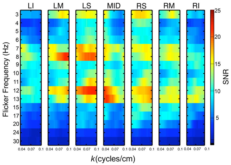
Spatial power spectra of the SSVEP obtained from the seven linear electrode arrays (see Fig. 2). Spatial power spectra are shown for each flicker frequency (3–30 Hz) over the wavenumber range 0.04–0.1 cycles/cm.

The SSVEP spatial power spectra show the highest power in the delta (f = 3 Hz), lower alpha (f = 7 and 8 Hz), and upper alpha (f = 11, 12, and 13 Hz) frequency bands, consistent with the maxima of potential SSVEP power (see Figure 4). Very little power is observed in the middle alpha frequency band (f = 9–10 Hz) in our limited wavenumber band; evidently most SSVEP source distributions occur at higher wavenumbers (not calculated for Figure 8), as evidenced by the strong Laplacian SSVEPs at these frequencies (see Figure 5). The spatial power spectra exhibit maximum power in a wavenumber range that depends on both the flicker frequency and electrode array location. At f = 3 Hz very little power is evident in the midline electrodes (MID), and the superior arrays of both hemispheres (LS and RS) show high power over a broad range of wavenumbers centered on k ~ 0.07 cycles/cm. The middle array of each hemisphere shows a narrower peak centered on k ~ 0.08 cycles/cm. The inferior arrays show very little power at any wavenumber in our range. In the lower alpha band (f = 7 or 8 Hz) the spatial power spectrum shows more power at the left hemisphere electrode arrays than the right hemisphere and less power at midline electrodes. In each array, the spatial spectra at f = 7 and 8 Hz are quite different, indicating the spatial distribution (and phases) of sources is modified by even a small change in the input frequency. With the LM and LS arrays, maximum power occurs at a wavenumber band centered on k ~ 0.08 cycles/cm at f = 8 Hz, while stronger power is evident at lower wavenumbers, centered on k ~ 0.05 cycles/cm at f = 7 Hz. Over the right hemisphere slightly higher power is observed at lower wavenumbers for f = 7 Hz compared to f = 8 Hz; the power differences are smaller than over the left hemisphere.

The spatial power spectra in the upper alpha band (f = 11, 12, and 13 Hz) also exhibit striking differences for small changes in the input frequency. At f = 11 Hz the power is concentrated in a narrow wavenumber band centered on k ~ 0.08 cycles/cm. At f = 12 Hz the spatial spectra indicate higher power over the left hemisphere than over the right hemisphere and broadly distributed over wavenumbers in the range shown; in each array maximum power is centered on k ~ 0.08 cycles/cm. At f = 13 Hz the highest power is observed with the midline array and simply falls off with increasing wavenumber. In the lateral arrays of both hemispheres, similar magnitude peaks in the wavenumber spectrum are narrower than at f = 12 Hz, and are centered on k ~ 0.08 cycles/cm in the arrays over the left hemisphere. Over the right hemisphere, power is distributed broadly over lower and higher wavenumbers; the response at lower wavenumbers extends to the most inferior array.

These results can be interpreted by comparison to the simulated spatial spectrum of a single dipole source (radial or tangential) where power simply falls off with increasing wavenumber (Figure 6), in a manner similar to both simulated white-noise source distributions and actual EEG noise (Figure 7). The main feature of the spatial spectrum of EEG noise is fall-off with increasing spatial frequency reflecting volume conduction. Since we normalize the SSVEP spatial power spectrum by the EEG noise spatial power spectrum, we expect that if the sources of the SSVEP are either a single dipole or a spatial white-noise, the normalized spatial power spectra will be nearly constant. Only the midline array exhibits a simple fall-off with increasing wavenumber at most frequencies, potentially indicating a single source region of finite size, i.e., a single dipole layer, rather than a point dipole source. However, in this array, the maximum power is observed at f = 13 Hz, and the fall-off in power with increasing wavenumber depends strongly on flicker frequency, suggesting at least some differences in the spatial extent of the source region with changes in input frequency. Furthermore, it may also be the case that midline electrodes are dominated by very long-wavelength source distributions (k < 0.04 cycles/cm), as suggested by the strong power in the potentials at midline electrodes over frontal areas.

The lateral arrays in both hemispheres exhibit peaks with finite bandwidth in the spatial power spectrum, which can only be accounted for by the presence of multiple source regions. In many cases peaks are observed near k ~ 0.08 cycles/cm corresponding to a wavelength of 12.5 cm, less than half the length of the anterior-posterior arrays. Peak power at this wavelength would not have been anticipated with a single (zero-phase lag) source region. The peaks are necessarily broad because of limitations in sampling at the scalp; even at the highest wavenumber (k = 0.1 cycles/cm) investigated here, only three spatial cycles of the wave are observed using our electrode array, severely limiting wavenumber resolution.

Wavenumber spectra of the SSVEP. Standing and traveling waves

Figure 9 shows the difference in power between experimental spectra evaluated at positive and negative wavenumbers for each one-dimensional array shown in Figure 2, taken at the frequencies that exhibited peak responses in the spatial power spectra shown in Figure 8. For each wavenumber k, the magnitude of the power difference between negative (back to front) and positive (front to back) waves is represented by the circle radius. Wavenumbers k where the difference between power at positive and negative k is less than 4.0 are set to zero radius (points). The sign of the difference is indicated by the circle color. Black circles indicate that higher power in negative wavenumbers (posterior-to-anterior waves) are dominant, and open circles indicate that positive wavenumbers (anterior-to-posterior) waves are dominant. Differences were considered significant if they exceeded 4.0. Since power is expressed in SNR units, this corresponds to four times the 95% confidence estimate of the noise and is very unlikely to be due to differences in additive noise at positive and negative wavenumbers.

Figure 9.

Difference between the power at negative and positive wavenumbers for the peak response flicker frequencies (f = 3,7 8,11,12, and 13 Hz). Differences were averaged across 9 subjects. For each frequency the difference in wavenumber spectrum Ψ(f, −k) − Ψ(f, + k) is shown at each wavenumber k by a point. Filled circles indicates a positive difference (posterior to anterior traveling waves) and open circles indicate a negative difference (anterior to posterior traveling waves). The size of each circle is proportional to the SNR difference. To emphasize robust differences larger than additive effects of broadband noise, any difference of magnitude less than 4.0 (in SNR units) was represented by a point. For example, the left superior (LS) array indicates anterior to posterior traveling 11 Hz waves of relatively long wavelengths. By contrast, this same array indicates 12 Hz posterior to anterior waves in roughly the same wave length range (10–15 cm).

The strongest evidence for traveling waves was found (off midline) at frequencies in the upper alpha band (f = 11, 12, and 13 Hz). At f = 13 Hz, at the midline electrodes the pattern resembles a standing wave with equal power at positive and negative wavenumbers across the whole band. By contrast, lateral electrodes over left and right hemispheres indicate strong evidence of traveling waves (large black circles). In the right hemisphere, posterior-anterior traveling waves are strongest in the right middle array (RM) with wavenumbers k ranging from 0.04 to 0.08 cycles/cm or wavelengths λ ranging from 12 to 25 cm. The far left hemisphere array (LI) also indicates traveling waves which are most evident at low wavenumbers (k < 0.07 cycles/cm). The strongest evidence of traveling waves occurs at higher wavenumbers k ranging from about 0.06 to 0.1 (λ ranging from 10–16 cm) in the superior array.

At f = 12 Hz, the pattern is qualitatively similar to the 13 Hz pattern; all traveling waves are in the posterior-to-anterior direction. The main difference is the absence of traveling waves in the right middle (RM) array at smaller wavenumbers; traveling waves are stronger in the left superior array (LS). At f = 11 Hz the right hemisphere shows a narrow wavenumber range of traveling waves similar to f = 12 or 13 Hz. The left hemisphere shows an entirely different pattern from that at 12 and 13 Hz with robust evidence of anterior to posterior waves at higher wavenumbers (short wavelengths). Another difference between temporal frequency bands is that midline electrodes show 11 Hz traveling waves in a narrow band centered on k ~ 0.06 cycles/cm.

At f = 3, 7, and 8 Hz, we find only minimal evidence of significant differences between positive and negative wavenumbers; standing wave patterns are more evident at most wavenumbers. The difference between positive and negative wavenumbers shown is always less than five times the noise level. Only very minimal evidence of traveling waves is observed in the midline electrodes at all flicker frequencies. Perhaps this is not surprising since midline electrodes are expected to record a roughly equal mixture of source activity from the two hemispheres.

DISCUSSION

SSVEPs are nearly always detected at occipital EEG electrodes or MEG sensors for a broad range of physical properties of the flickering stimulus (including its temporal and spatial frequency content). In this study, we demonstrate that in regions far from primary visual cortex, the SSVEP dynamic response is a sensitive function of flicker frequency. In each frequency band, scalp EEG power depends on the location, strength, and relative phases of cortical dipole sources (Nunez and Srinivasan, 2005). Since the physical properties of the flickering stimulus are held constant, we may reasonably expect that small (1–2 Hz) changes in flicker frequency will not change the spatial location of inputs to striate cortex (Silberstein, 1995). Thus, the observed changes in SSVEP dynamic response with changes in flicker frequency are much more likely to reflect dynamic properties of cortical sources. Both the spatial and temporal properties of the source dynamics observed with scalp potentials apparently depend strongly on input frequency. By applying the surface Laplacian algorithm to scalp potentials, we spatially filter the raw data and demonstrate that the responses of the more localized sources in occipital and parietal cortex are strongly frequency dependent; different input frequencies elicit Laplacian peaks at different electrodes. In addition to the patterns of localized sources that depend critically on input frequency, large-scale source distributions spanning anterior and posterior cortical regions contribute to the SSVEP especially at frontal electrodes. The large-scale responses are also critically dependent on input frequency. These distributed sources exhibit magnitude and phase patterns that appear to be standing and traveling waves at the input frequency.

Source Localization of the SSVEP

Source localization of the SSVEP has been used to describe how the “center” of activity in occipital cortex varies as a function of physical properties of the flicker and cognitive processes such as attention. A few (or even just one) isolated dipole sources in visual cortex have been proposed to account for the spatiotemporal properties of the SSVEP or SSVEF (Okada et al., 1982; Maier et al., 1987; Muller et al., 1997). The dipole approximation to cortical current sources provides the basis for most source models of EEG signals (Lopes da Silva, 2004; Nunez and Srinivasan, 2005). It is based on the idea that at large distances, any complex current distribution in a region of the cortex can be approximated by dipole moment per unit volume. A “large” distance is at least 3 or 4 times the pole separation within the volume. Superficial gyral surfaces of the cortex are located at roughly 1.5 cm from scalp electrodes. Thus for superficial tissue, the dipole approximation appears valid for a cortical volume with extent (in any direction) of less than 0.5 cm, which is roughly the diameter of a macrocolumn in visual cortex (Mountcastle, 1997), or the typical size of a voxel in functional Magnetic Resonance Imaging (fMRI). Thus, genuine source distributions underlying EEG signals are more accurately described as dipole layers. For instance a superficial gyral crown of surface area 2 cm² is more accurately described as a small dipole layer composed of multiple active dipole sources. More generally, dipole moment per unit volume can be considered a continuously varying function of cortical location. Very localized sources are just extreme cases where dipole moment is very large over a compact region of the cortex and much lower everywhere else. If these “localized” source regions are superficial, they can be easily detected with surface Laplacian methods.

Surface Laplacian SSVEPs

The surface Laplacian provides a clearly interpretable estimate of the contribution of “localized” source activity to the SSVEP. At occipital and parietal electrodes, surface Laplacian-based SSVEPs exhibit robust responses at each flicker frequency, and the spatial distribution of this response depends strongly on flicker frequency. The implication is that the source magnitudes in small dipole layers (with zero phase lag among the dipoles) in occipital and parietal cortex are exquisitely sensitive to input frequency. Different input frequencies result in different patterns of magnitude and phase over occipital cortex, which can sum or cancel at the scalp electrodes, depending on their location. At f = 8 and 10 Hz, such small dipole layers are also detected outside of occipital and parietal cortex, including sites over frontal areas.

By contrast, the robust frontal responses observed in the potential SSVEP at f = 3, 7, 8, 12, and 13 Hz are not apparent with the surface Laplacian. This negative result has a clear interpretation: sources that contribute to the frontal SSVEP at these frequencies are either deep or broad (diameter > 5–7 cm). Such source activity is unlikely to simply reflect volume conduction of occipital source activity; one strong argument against this interpretation is that occipital potential SSVEPs show very little spatial variability between flicker frequencies, but the spatial patterns of the frontal potential SSVEPs are critically dependent on flicker frequency. The question of a deep tangential source versus a broad superficial dipole layer is addressed in part by the wavenumber spectrum results discussed below, which suggest a distributed source configuration spanning occipital, parietal, and frontal lobes.

SSVEP waves

In addition to the local sources mainly in occipital and parietal lobes, we observed apparent large-scale source activity spanning both posterior and anterior regions of the array. We characterized the dynamics of this long-wavelength source activity with spatial power spectra and wavenumber spectra in one-dimensional arrays running from posterior (occipital/parietal) to anterior (prefrontal) electrodes. Our motivation for using one-dimensional arrays oriented along anterior-posterior directions was two fold: (1) although the scalp surface maybe fit to a sphere, and spherical harmonic decompositions have been applied to EEG data (Wingeier et al., 2004), each cerebral hemisphere is better described as an ellipsoid with the long axis oriented in the anterior-posterior direction. (2) From a physiological viewpoint, dipole moment per unit volume is more reasonably modeled as a continuous function of location within each neocortical hemisphere. Although callosal fibers connect homologous regions of the visual system; cortical tissue is not continuous over the boundary between the two hemispheres. The choice of one-dimensional spectra has limitations; each cerebral hemisphere is a two-dimensional surface along which waves can travel in any direction. However, even a two-dimensional spatial spectral analysis based on scalp surface electrode position is only an approximation to the spatial spectra in the cortex.

The spatial power spectra over the wavenumber range 0.04 to 0.1 cycles/cm provide a partial picture of spatial properties of the underlying large-scale sources. If either a single source or spatial white noise source distributions were to generate the SSVEP, the spatial spectra would simply fall-off with wavenumber, as observed in both simulations and EEG noise estimates. By contrast, we found peaks in the spatial power spectra of the SSVEP data that depended critically on both the flicker frequency and location of the linear electrode array. These peaks can only be explained by distributed sources forming two or more source regions with different phases.

Furthermore, we found power differences between positive and negative wavenumbers for flicker frequencies in the upper alpha band. The sign of the wavenumber indicates the direction of propagation (increasing phase) in the array. At f = 12 and 13 Hz we found evidence of both long wavelength (~ 15–25 cm) and short wavelength (~10–12 cm) waves propagating from posterior to anterior regions of the array. At f = 11 Hz we found evidence of short wavelength waves propagating from anterior to posterior electrodes. By contrast, only limited evidence of traveling waves was observed at the other flicker frequencies of that we studied; the spatial patterns of phase were consistent with standing waves. Thus, we found robust evidence that some distributed sources are characterized by patterns of amplitude and phase that share properties of wave propagation. The wave dynamics depends strongly on the input frequency.

Physiological Implications

The observations of this study are consistent with the physiological literature on the organization of the visual system (Felleman and Van Essen, 1991). The existence of a single generator of the SSVEP would not be predicted by the functional anatomy of the visual system. Input to primary visual cortex (V1) is distributed via corticocortical fiber systems to higher areas (V2, V3, V4, V5, etc.), which in turn provide feedback to primary visual cortex. In a typical SSVEP recording the stimulus flicker is presented for a very long duration (50s in this experiment), implying the input is being processed in distributed cortical networks. The dynamics of these networks depends in part on propagation delays in white-matter axons, which introduces phase differences between sources. Just within the monkey visual cortex, delays on the order 20–35 ms have been observed (Schmolesky et al., 1998), and the estimated delays in long-range (e.g., anteriorposterior) white-matter fibers can be greater than 30–50 ms (Nunez, 2000).

Conscious perception of the flicker increases the coherence of these responses over distant cortical sites (Srinivasan et al., 1999; Srinivasan, 2004), possibly reflecting recursive signaling within large-scale distributed cortical networks predicted by theoretical models of conscious experience (Edelman, 1999). Thus, the cortical sources underlying the SSVEP may be distributed over the whole brain, with phase determined partly by propagation delays, and apparently including source distributions in the frontal lobes. SSVEP sources apparently are organized over multiple spatial scales including relatively localized scales (2–3 cm) primarily in the occipital and parietal lobes and regional or even global scales. Apparently, the dynamics of the source distributions exhibit different sensitivity to temporal frequency at different spatial scales.

Connections to neocortical dynamic theory

Known physical wave phenomena generally consist of wave packets, often containing a broad range of wave components having different spatial wavelengths. The phase velocity of any traveling wave component within such a packet with spatial wavelength λ and temporal frequency f is given by

$$v_P=\lambda f$$ (7)

The most robust of the putative traveling waves observed in our SSVEP data have phase velocities in the 1 to 3 m/s along the scalp or about 2 to 6 m/s along the folded cortical surface. In this study, we did not attempt to estimate phase velocities for possible waves with shorter or longer wavelengths than were dictated by our linear electrode arrays. However, other studies of SSVEP using close bipolar electrodes and MEG and have estimated that the bulk of ~10 Hz SSVEP phase velocities along the cortical surface is in the 4 to 12 m/s range (Silberstein, 1995; Nunez, 1995, Burkitt et al., 2000). The difference between these velocity range estimates can be attributed to differences in the analysis methods. In the studies cited above, linear regression analysis was applied to the spatial change in phase with distance in the electrode array in a single ~10 Hz frequency band. Such estimates are likely to be dominated by very long wavelengths, which are emphasized at each electrode because of volume conduction effects. Furthermore, other studies have shown that, aside from volume conduction effects, wavenumber spectral power exhibits minima within the alpha band of spontaneous EEG, in other words spontaneous alpha band rhythms have, on average, the longest wavelengths (Nunez 1995; Wingeier 2001). It is not now clear how well this observation of spontaneous EEG dynamics applies to SSVEP’s. Our tentative conclusion is that the 10 Hz flicker used in our study fails to drive the global alpha rhythm and instead drives multiple local alpha rhythms. The evidence here for driven global rhythms is stronger in the low (7–8 Hz) and high alpha (12–13 Hz) bands. These observations are, of course, dependent on the physical stimulus, task, and subject. In other experiments (Ding et al., 2005; Srinivasan et al., 2004) strong global responses are driven in the middle of the alpha band (9 and 10 Hz).

One reason for experimental bias towards longer wavelengths when using linear regression of phase has to do with phase ambiguity when phase changes are too large over progressive array locations. Nevertheless, such estimates are valid over their appropriate wavenumber range. These long-wavelength estimates reasonably match estimates of corticocortical propagation speeds. Such speeds are distributed, but the bulk of fibers are estimated to produce speeds in the 6 to 9 m/s range (Nunez, 1995). In our study, wavelengths longer than the electrode array were not examined; spatial Fourier methods are suited only to a shorter wavelength range. Also, a broader range of temporal frequencies is examined here compared to previous studies of SSVEP spatial properties, and we obtain somewhat lower estimates of phase velocity.

One approach to neocortical dynamic theory (Nunez, 1981, 1989, 1995, 2000a,b; Nunez and Srinivasan 2005) suggests that EEG (and by implication SSVEP) is composed of some combination of local and global dynamic processes. That is, local networks are pictured as immersed in global synaptic action fields, In this local-global theory local processes are mainly due to intracortical and thalamocortical interactions, whereas global processes are due largely to corticocortical interactions. Globally generated waves of long wavelength are predicted to propagate through the cortical-white matter system over a range of speeds that can be broad or narrow depending on brain state; however, predicted speeds are in the general range of corticocortical propagation speeds. Thus, the SSVEP data presented here are qualitatively consistent with two essential features of the local-global dynamic theory cited above: (1) the existence of both localized and distributed source distributions that may operate in either distinct or overlapping temporal frequency bands. (2) the prediction of traveling waves with speeds in the general range of corticocortical propagation speeds. Qualitatively similar experimental results have been reported for spontaneous EEG (Nunez 1995; Nunez et al, 2001; Wingeier et al., 2001).

CONCLUSIONS

In this study we have provided empirical evidence of dynamic, distributed source configurations underlying the SSVEP. These sources are organized at both small spatial scales (2–3 cm) and large-spatial scales (10–25 cm). Spatial properties of SSVEP sources depend strongly on input frequency. Simple models of the SSVEP based on, for example, one source in the occipital lobe are clearly inadequate to explain the patterns of organization of SSVEP magnitude and phase. The development of theoretical models of the generators of the SSVEP should apparently include many local sources in occipital, parietal, and even frontal cortex, and large-scale generator regions that give rise to standing and traveling wave dynamics.

References

- Bertrand O, Perrin F, Pernier J. A theoretical justification of the average-reference in topographic evoked potential studies. Electroencephalogr Clin Neurophysiol. 1985;62:462–464. doi: 10.1016/0168-5597(85)90058-9. [DOI] [PubMed] [Google Scholar]
- Bertrand O, Perrin F, Pernier J. A theoretical justification of the average reference in topographic evoked potential studies. Electroenceph clin Neurophysiol. 1986;62:462–464. doi: 10.1016/0168-5597(85)90058-9. [DOI] [PubMed] [Google Scholar]
- Brainard DH. The Psychophysics Toolbox. Spatial Vision. 1997;10:433–436. [PubMed] [Google Scholar]
- Burkitt GR, Silberstein RB, Cadusch PJ, Wood AW. The steady-state visually evoked potential and travelling waves. Clinical Neurophysiology. 2000;111:246–258. doi: 10.1016/s1388-2457(99)00194-7. [DOI] [PubMed] [Google Scholar]
- Chen Y, Seth AK, Gally JA, Edelman GM. The power of human brain magnetoencephalographic signals can be modulated up or down by changes in an attentive visual task. Proc Natl Acad Sci U S A. 2003;100:3501–6. doi: 10.1073/pnas.0337630100. [DOI] [PMC free article] [PubMed] [Google Scholar]
- Ding J, Sperling G, Srinivasan R. SSVEP power modulation by attention depends on the network tagged by the flicker frequency. Cerebral Cortex. 2005 doi: 10.1093/cercor/bhj044. in press. [DOI] [PMC free article] [PubMed] [Google Scholar]
- Edelman GM. Building a picture of the brain. Ann N Y Acad Sci. 1999;882:68–89. doi: 10.1111/j.1749-6632.1999.tb08535.x. [DOI] [PubMed] [Google Scholar]
- Felleman DJ, Van Essen DC. Distributed hierarchical processing in the primate cerebral cortex. Cerebral Cortex. 1991;1:1–47. doi: 10.1093/cercor/1.1.1-a. [DOI] [PubMed] [Google Scholar]
- Law SK, Nunez PL, Wijesinghe RS. High-resolution EEG using spline generated surface Laplacians on spherical and ellipsoidal surfaces. IEEE Trans Biomed Eng. 1993;40:145–53. doi: 10.1109/10.212068. [DOI] [PubMed] [Google Scholar]
- Lopes da Silva F. Functional localization of brain sources using EEG and/or MEG data: volume conductor and source models. Magn Reson Imaging. 2004;22:1533–8. doi: 10.1016/j.mri.2004.10.010. [DOI] [PubMed] [Google Scholar]
- Maier J, Dagnielie G, Spekreijse H, van Dijk BW. Principal components analysis for source localization of VEPs in man. Vision Research. 1987:165–177. doi: 10.1016/0042-6989(87)90179-9. [DOI] [PubMed] [Google Scholar]
- McDonough RN. Application of maximum likelihood and maximum entropy method to array processing. In: Haykin S, editor. Nonlinear methods of spectral analysis. Springer Verlag; 1988. [Google Scholar]
- Mountcastle VB. Perceptual Neuroscience: The Cerebral Cortex. Academic Press; NY: 1997. [Google Scholar]
- Muller MM, Teder W, Hillyard SA. Magnetoencephalographic recording of steady-state visual evoked cortical activity. Brain Topography. 1997;9:163–168. doi: 10.1007/BF01190385. [DOI] [PubMed] [Google Scholar]
- Nakayama K, Mackeben M. Steady-state visual evoked potentials in the alert primate. Vision Research. 1982;22:1261–1271. doi: 10.1016/0042-6989(82)90138-9. [DOI] [PubMed] [Google Scholar]
- Narici L, Portin K, Salmelin R, Hari R. Responsiveness of human corical activity to rhythmical stimulation: A three-modality, whole-cortex neuromagnetic investigation. 1998;7:209–223. doi: 10.1006/nimg.1998.0323. [DOI] [PubMed] [Google Scholar]
- Nunez PL. Wavelike properties of the alpha rhythm. IEEE Transactions on Biomedical Engineering. 1974;21:473–482. [Google Scholar]
- Nunez PL. Electric Fields of the Brain: The Neurophysics of EEG. 1. New York: Oxford UP; 1981. [Google Scholar]
- Nunez PL. Generation of human EEG by a combination of long and short range neocortical interactions. Brain Topography. 1989;1:199–215. doi: 10.1007/BF01129583. [DOI] [PubMed] [Google Scholar]
- Nunez PL. Neocortical Dynamics and Human EEG Rhythms. New York: Oxford University Press; 1995. [Google Scholar]
- Nunez PL. Toward a quantitative description of large scale neocortical dynamic function and EEG. Behavioral and Brain Sciences. 2000a;23:415–437. doi: 10.1017/s0140525x00003253. (Invited target article) [DOI] [PubMed] [Google Scholar]
- Nunez PL. Neocortical dynamic theory should be as simple as possible, but not simpler. Behavioral and Brain Sciences. 2000b;23:371–398. doi: 10.1017/s0140525x00003253. (Response to 18 commentaries by neuroscientists on target article) [DOI] [PubMed] [Google Scholar]
- Nunez PL, Srinivasan R. Electric Fields of the Brain: The Neurophysics of EEG. 2. New York: Oxford UP; 2005. [Google Scholar]
- Nunez PL, Silberstein RB, Cadusch PJ, Wijesinghe RS, Westdorp AF, Srinivasan R. A theoretical and experimental study of high-resolution EEG based on surface Laplacians and cortical imaging. Electroencephalography and Clinical Neurophysiology. 1994;90:40–57. doi: 10.1016/0013-4694(94)90112-0. [DOI] [PubMed] [Google Scholar]
- Nunez PL, Srinivasan R, Westdorp AF, Wijesinghe RS, Tucker DM, Silberstein RB, Cadusch PJ. EEG coherency. I: Statistics, reference electrode, volume conduction, Laplacians, cortical imaging, and interpretation at multiple scales. Electroencephalogr Clin Neurophysiol. 1997;103:499–515. doi: 10.1016/s0013-4694(97)00066-7. [DOI] [PubMed] [Google Scholar]
- Nunez PL, Wingeier BM, Silberstein RB. Spatial-temporal structure of human alpha rhythms: Theory, microcurrent sources, multiscale measurements, and global binding of local networks. Human Brain Mapping. 2001;13:125–164. doi: 10.1002/hbm.1030. [DOI] [PMC free article] [PubMed] [Google Scholar]
- Okada YC, Kaufman L, Brenner D, Williamson SJ. Modulation transfer functions of the human visual system revealed by magnetic measurements. Vision Research. 1982;22:319–333. doi: 10.1016/0042-6989(82)90132-8. [DOI] [PubMed] [Google Scholar]
- Perrin F, Bertrand O, Pernier J. Scalp current density mapping: value and estimation from potential data. IEEE Trans Biomed Eng. 1987;34:283–287. doi: 10.1109/tbme.1987.326089. [DOI] [PubMed] [Google Scholar]
- Perrin F, Pernier J, Bertrand O, Echallier JF. Spherical spline for potential and current density mapping. Electroenceph clin Neurophysiol. 1989;72:184–187. doi: 10.1016/0013-4694(89)90180-6. [DOI] [PubMed] [Google Scholar]
- Rager G, Singer W. The response of cat visual cortex to flicker stimuli of variable frequency. European J of Neuroscience. 1998;10:1856–1877. doi: 10.1046/j.1460-9568.1998.00197.x. [DOI] [PubMed] [Google Scholar]
- Regan D. Steady-state evoked potentials. J Opt Soc Am. 1977;67:1475–89. doi: 10.1364/josa.67.001475. [DOI] [PubMed] [Google Scholar]
- Regan D. Human brain electrophysiology. New York: Elsevier; 1989. [Google Scholar]
- Schmolesky MT, Wang Y, Hanes DP, Thompson KG, Leutgeb S, Schall JD, Leventhal AG. Signal timing across the macaque visual system. Journal of Neurophysiology. 1998;79:3272–3278. doi: 10.1152/jn.1998.79.6.3272. [DOI] [PubMed] [Google Scholar]
- Silberstein RB, Nunez PL, Pipingas A, Harris P, Danieli F. Steady state visually evoked potential (SSVEP) topography in a graded working memory task. International Journal of Psychophysiology. 2001;42:219–232. doi: 10.1016/s0167-8760(01)00167-2. [DOI] [PubMed] [Google Scholar]
- Silberstein RB. Steady-state visually evoked potentials, brain resonances, and cognitive processes. In: Nunez PL, editor. Neocortical Dynamics and Human EEG Rhythms. Oxford University Press; 1995. pp. 272–303. [Google Scholar]
- Silberstein RB, Danieli F, Nunez PL. Fronto-parietal evoked potential synchronization is increased during mental rotation. NeuroReport. 2003;14:67–71. doi: 10.1097/00001756-200301200-00013. [DOI] [PubMed] [Google Scholar]
- Silberstein RB, Song J, Nunez PL, Park W. Dynamic sculpting of brain functional connectivity is correlated with performance measures. Brain Topography. 2004;16:249–254. doi: 10.1023/b:brat.0000032860.04812.b1. [DOI] [PubMed] [Google Scholar]
- Sperkeijse H, Estevez O, Reits D. Visual evoked potentials and the physiological analysis of visual processes in man. In: Desmedt JE, editor. Visual evoked potentials in man: new developments. Clarendon Press; Oxford: 1977. pp. 16–89. [Google Scholar]
- Srinivasan R, Nunez PL, Tucker DM, Silberstein RB, Cadusch PJ. Spatial sampling and filtering of EEG with spline Laplacians to estimate cortical potentials. Brain Topography. 1996;8:355–366. doi: 10.1007/BF01186911. [DOI] [PubMed] [Google Scholar]
- Srinivasan R, Nunez PL, Silberstein RB. Spatial filtering and neocortical dynamics: estimates of EEG coherence. IEEE Transactions on Biomedical Engineering. 1998;45:814–826. doi: 10.1109/10.686789. [DOI] [PubMed] [Google Scholar]
- Srinivasan R, Russell DP, Edelman GM, Tononi G. Increased synchronization of neuromagnetic responses during conscious perception. Journal of Neuroscience. 1999;19(13):5435–5448. doi: 10.1523/JNEUROSCI.19-13-05435.1999. [DOI] [PMC free article] [PubMed] [Google Scholar]
- Srinivasan R. Internal and external neural synchronization during conscious perception. International Journal of Bifurcation and Chaos. 2004;19:1–18. doi: 10.1142/S0218127404009399. [DOI] [PMC free article] [PubMed] [Google Scholar]
- Srinivasan R, Petrovic S. MEG phase follows conscious perception during binocular rivalry induced by visual stream segregation. Cerebral Cortex. 2005 doi: 10.1093/cercor/bhj016. in press. [DOI] [PMC free article] [PubMed] [Google Scholar]
- Tyler CW, Apkarian P, Nakayama K. Multiple spatial frequency tuning of electrical responses from the human visual cortex. Experimental Brain Research. 1978;33:535–550. doi: 10.1007/BF00235573. [DOI] [PubMed] [Google Scholar]
- Wingeier BM, Nunez PL, Silberstein RB. Spherical harmonic decomposition applied to spatial-temporal analysis of human high-density electroencephalogram. Physical Review E. 2001;64:051916-1–9. doi: 10.1103/PhysRevE.64.051916. [DOI] [PubMed] [Google Scholar]