MEG phase follows conscious perception during binocular rivalry induced by visual stream segregation

Abstract

We have investigated an unusual form of binocular rivalry between two images that are flickered one to each eye, but are never presented simultaneously to the observer. The images are presented in alternation, with a brief dark period between the images. When the flicker frequency was below 5 Hz, the subjects primarily experienced a unitary flicker that alternated between the two images. When the flicker frequency was above 5 Hz, the subjects primarily experienced two single-image flickers that rival. We investigated MEG responses at the flicker frequency of the rival stimuli. We found that at some recording locations responses are phase-locked to the flicker that is consciously being perceived. At each flicker rate that induced rivalry, phase shifts following the conscious percept were found consistently at MEG sensors over midline frontal lobe. Most of these sensors show higher magnitude responses when two rivaling flickers are perceived than when a unitary alternating color flicker is perceived. At sensors over occipital lobe, the sensor locations that phase-locked to the perceived flicker depended on the color, orientation, and frequency of flicker. Apparently, a large-scale network of cell assemblies in occipital and frontal cortex, responds preferentially to the perceived stimulus during rivalry, and is sensitive to the timing of the flicker driving the conscious percept.

Introduction

In binocular rivalry, two incongruent visual images are simultaneously presented to the observer, one to each eye. The observer reports spontaneous episodes of stable perception of only one image. A number of studies have shown that the distribution of durations of reported episodes of perceptual dominance of one image generally resembles a gamma distribution (Fox and Herrmann 1967; Levelt 1967; Blake, Fox et al. 1971). The timing and duration of perceptual reports depend on physical aspects of the stimuli, such as spatial and temporal frequency, orientation, contrast, and chromaticity. (Fahle 1982; Wolfe 1983; O’Shea and Crassini 1984; Mueller and Blake 1989). Since no stimulus manipulation is needed to induce spontaneous perceptual dominance of one stimulus (and the suppression of the rival stimulus), binocular rivalry has been used in a number of neurophysiological studies to identify aspects of cortical dynamics related to conscious visual perception in both humans and animal models (Leopold and Logothetis 1996; Fries, Roelfsema et al. 1997; Tong, Nakayama et al. 1998; Lumer and Rees 1999; Srinivasan, Russell et al. 1999; Blake and Logothetis 2002).

Binocular rivalry also occurs if the stimuli are presented simultaneously, but intermittently (Wolfe 1983). With short dark intervals, rivalry was still observed. Rivalry between stimuli flickered synchronously at 18 Hz (Logothetis, N et al. 1996) resembles conventional rivalry. Rivalry persists even if the synchronously flickered images are switched between the eyes every 333 ms, which supports the notion that this rivalry can take place between percepts in addition to rivalry between eyes (Lee and Blake, 1999). When the two rival stimuli are flickered asynchronously at two different frequencies above 7 Hz, the perceptual reports of observers are qualitatively similar to those reported during the static presentation of the rival images, despite the fact that the subject is presented two intermittent stimuli (Srinivasan, Russell et al. 1999; Srinivasan 2004). Interstimulus intervals are variable throughout the stimulus presentation, and the two images are superimposed only at the beat frequency between the two stimulus flickers. Thus, the stimuli are not always presented simultaneously to each eye, nor are the intervals between the stimuli regular. Rivalry still takes place, with dominance periods on the order of 2 secs, similar to rivalry with static images.

O’Shea and Crassini (1984) have demonstrated that binocular rivalry can occur even when the rivaling stimuli are never presented simultaneously, but instead alternated at a fixed interstimulus interval (ISI), which they termed successive binocular rivalry. In this experiment, rivalry was reported by three observers, even when one of the stimuli is briefly presented for 5ms, followed by a dark screen for over 100ms, followed by the rival stimulus for 5 ms in a train of stimulation. Thus, each stimulus was flickered into each eye at the same frequency (f_R), but the two eyes were stimulated 180° out of phase. Rivalry was reported for flicker frequencies as low as f_R = 3Hz. Interestingly, this identical limit has also been reported as the Gestalt flicker frequency (van de Grind et al., 1973), that is, the lowest frequency at which a repeating stimulus is perceived as flicker. Subjects’ reports of rivalry under experimental conditions where the rival stimuli were flickered out of phase were indistinguishable from conditions where the rival stimuli were flickered simultaneously (in phase) at the same rate for f_R > 5 Hz.

This effect has some qualitative similarities to the phenomenon of auditory stream segregation studied extensively by Bregman (Bregman 1990). In a typical auditory streaming experiment, the stimuli consist of alternating high and low frequency tones. Depending on the duration of the tones, the stimulus train can either be perceived as a single percept of alternating high and low tones, or two independent streams, one repeating high tone and one repeating low tone. In the visual experiment of O’Shea and Crassini (1984) alternating incongruent visual stimuli (orthogonal gratings) are either perceived as one flicker with alternating orientation or as two distinct flickers with different orientations. The main difference is that in the visual experiment the two flickers, which are never coincident, appear to rival. During auditory stream segregation both repeating tones are perceived simultaneously, and there is no competition between percepts, although attention can be used to enhance or suppress one of the auditory streams. Motivated by this partial analogy, we refer to the phenomena reported by O’Shea and Crassini (1984) as binocular rivalry induced by visual stream segregation. Our primary goal was to confirm the results of O’Shea and Crassini (1984) and use this display to identify neural correlates of conscious perception during rivalry using steady-state MEG recordings in human subjects.

In earlier “frequency-tagging” studies of rivalry (Srinivasan et al., 1999; Srinivasan et al., 2004), steady-state brain responses two two incongruent stimuli flickered at distinct frequencies were detected using EEG and MEG recordings. In these studies, steady-state responses appear not only over visual cortex, but also over parietal, temporal, and even frontal areas far from the visual system. Sensors over occipital cortex show responses at almost any flicker frequency; sensors at frontal and temporal locations only produced a robust response to flicker over narrow (1–2 Hz) ranges of flicker frequencies, usually in the theta or alpha bands. When the stimulus flicker was perceived, steady-state power was increased as compared to when the other stimulus flickered at a different frequency was perceived (Srinivasan, Russell et al. 1999; Srinivasan 2004). We observed the strongest effects on the steady-state response at temporal and frontal channels when the flicker was at an apparent “global” frequency in the alpha band, specific to each subject, that produces widespread responses over the entire array in both EEG and MEG recordings. We also observed increased coherence between frontal sensors and occipital/temporal sensors, both within and across hemispheres.

We could not easily observe whether the steady-state response to each flicker was modulated in opposite directions (following the subjects reports) at any one sensor. The responses to two rival stimulus flickers (at different frequencies) intrinsically have different spatial distribution, as a consequence of the input frequency selecting for different cortical networks that can synchronize to the flicker. The only sensors that consistently show response at two different frequencies are located over occipital and parietal cortex. At these occipital/parietal sensors, the effect of rivalry on MEG power was much smaller than at frontal or temporal sensors (Srinivasan et al., 1999). We often found a response to only one of the two flickers was detected at many temporal and frontal sensors.

In this study, we investigate whether switches in conscious perception between two flickers is associated with switches in the dominance of steady-steady responses to each flicker at one MEG sensor using a display modeled after O’Shea and Crassini (1984). In this experiment, as in the study by O’Shea and Crassini (1984), two incongruent stimuli are flickered (one to each eye) at the same frequency, but out of phase. In this design, the spatial distribution of the MEG signals induced by each of the rival stimuli are expected to be similarly influenced by the choice of flicker frequency. We examined the steady-state MEG response to determine where we can detect phase changes between episodes of conscious perception one single-image flicker versus perception of the other single-image flicker. We hypothesized that a subset of MEG sensors will exhibit 180 degree phase shifts corresponding to the physical difference between rival flickers, as a consequence of phase-locking of cortical networks to the consciously perceived flicker.

Materials and methods

Stimuli

Two incongruent images were presented dichoptically, intermittently, and out of phase, as shown by the example in Figure 1. The two incongruent images were horizontal and vertical square wave gratings within a static fusing annulus present throughout the trial. One grating was red and the other blue, presented one to each eye using corresponding color filters. There were always 4 trials used to counterbalance physical aspects of the stimuli (2 colors and 2 orientations) presented to each eye.

Figure 1. Stimulus properties.

A. Time courses of two incongruent, flickering gratings, as presented to the subject. Each grating is always presented to the same eye throughout a trial. One stimulus cycle (T) consists of a stimulus presentation (Δt ~13ms), followed by a much longer (120ms-254ms) dark interval, before the repeated stimulus occurrence. Both stimuli have the same repetition cycle T, but are never shown simultaneously. Instead, they are interleaved at exactly same inter-stimulus intervals (ISI), effectively making their presentations 180 degrees out of phase.

B. Throughout the experiment, we varied time courses of stimulus presentations by varying the stimulus cycle length T, while keeping Δt unchanged. This table summarizes 6 different values of T used in the experiment, along with the related measures of stimulus flicker frequency (f_R) and ISI. We refer to them interchangeably throughout the document (f_R = 1/T, ISI = T/2). The specific choice of values were irregular as they were multiples of the duration of a single video frame(~13ms, at 75Hz refresh rate

Stimuli were projected using a Proxima 4200 DLP projector driven by a G4 Macintosh, using programs written in MATLAB (Natick, MA) with Psychophysics Toolbox extensions (Brainard 1997; Pelli 1997). Flicker was produced using a vertical refresh rate of 75 Hz. Each stimulus image was presented for 1 video frame (duration ~ 13 ms), followed by a dark screen until the presentation of the rival stimulus. Each grating flickered at a constant flicker frequency f_R during a single trial, corresponding to the stimulus cycle interval T composed of one presentation of each of the rival stimuli (f_R = 1/T). Thus, on each trial both gratings flickered at the same frequency, but were presented 180° out of phase. A total of 6 different stimulus repetition rates were used, as summarized in the table (Fig. 1). This range of values was selected based on results of O’Shea and Crassini (1984), which showed that the number of reported episodes of perceptual dominance of one stimulus flicker grows with flicker frequency between 3 and 8Hz above which it remains constant, and comparable to static presentation of the two stimuli.

Stimulus was projected through a porthole to a mirror, and then to a screen located in front of the subject. The size of the projected stimulus was 12 cm in diameter, and was viewed at a distance of 57 cm. The stimulus, consisting of square gratings of 0.5 cycles/°, subtended a visual angle of 12°. Average luminance of the flickering stimulus after passing through the colored lenses was 0.02 cd/m².

Procedure

There were a total of 6 subjects, 4 males and 2 females. The experiment was undertaken with the understanding and written consent of each subject. All subjects were trained to report binocular rivalry dominance periods for different stimulus presentation rates. Each subject was presented with a total of 24 trials, where each trial lasted 100s.

Subjects were asked to fixate on a dim gray point at the center of the superimposed gratings. Subjects viewed the stimuli through red-blue filter glasses, and made keypad responses to report their percept. The responses consisted of pressing and holding one key during stable episodes of blue stimulus flicker, pressing and holding another key during stable episodes of red flicker, and pressing and holding both keys during alternating-color flicker. Subjects were instructed not to respond if they saw a mixture of red and blue patches that occurs during a transitional phase.

Control Experiments

Three control experiments were carried out on separate days after the rivalry experiment: (1) Monocular stimulation. Each stimulus flicker (red/blue and horizontal/vertical) was presented to each eye for 60 s, with a dark screen presented to the other eye. This control was obtained in 2 subjects. (2) Binocular congruent stimulation. Iso-oriented (both horizontal or both vertical) pairings of red and blue stimulus flicker were presented 180 degrees out of phase one to each eye for 60 s. This control experiment was carried out on the same day as the monocular stimulation. (3) Synchronous rivalry stimulation. Stimulus flicker conditions were identical to the rivalry experiment, but the rival flickers were presented synchronously with no phase difference between the two eyes. All combinations of pairings of stimulus (color and orientation) and eye were used identical to the rivalry experiment. This control experiment was carried out in 1 subject. MEG ProcedureNeuromagnetic data was collected using a Magnes 2500WH M EG system from Biomagnetic Technologies (San Diego, CA). This array provides coverage of the entire scalp by means of 148 magnetometer coils (1 cm in diameter) that are spaced 3 cm apart on an approximately ellipsoidal surface located ~ 3 cm from the scalp surface. The sampling rate of the acquired signals was 508 samples/sec. Estimated equipment and room noise was removed from the raw data by digital filtering, using reference coils positioned in the dewar above the array of MEG coils (Srinivasan et al., 1999). The data acquisition computer also detected and recorded timing of blue and red frame presentations by using photocell sensors.

High-resolution FFT Analysis of MEG signals

High-resolution steady-state responses were estimated by calculating Fourier transform F_m(f) of the entire ~100 s MEG recording, with the exact interval determined by the first and last presentation of the stimuli. The frequency resolution of this spectrum was ~ 0.01 Hz. From these Fourier coefficients, power spectrum at each channel was calculated as

$$P_m(f)=2\times F_m(f)\times F_m^{\ast }(f)$$ (1)

The same calculation was done for all 4 trials of the same flicker frequency, and their power values averaged. The signal-to-noise ratio (SNR) was calculated at each MEG channel as the ratio of power at the stimulus flicker frequency (f_R), and average power of 20 surrounding frequency bins (10 below and 10 above) that were at most 0.2 Hz away from f_R. Signal-to-noise ratio (SNR) was also estimated for each harmonic of the stimulus frequency up to the 5^th harmonic (5f_R).

Segmentation by perceptual reports

Data segmentation was performed strictly according to the stimulus presentation times recorded with a photocell. Each data segment had the length of one stimulus cycle (T), i.e. the length of time between two consecutive presentations of the same image. These cycle lengths were identical for the red and blue images, but out of phase. In order to obtain interpretable phase estimates, we always segmented such that the beginning and end of each segment was always aligned to the presentation of a blue image. Thus, the blue image was always presented at the start of each segment while the red image was always presented at the center of each data segment. Data segments were classified into 4 groups based on the perceptual reports given by the subjects: blue flicker dominant, red flicker dominant, alternating color flicker and mixed. Segments falling into the mixed category included both patchy rivalry (no response) and the transitional cycles at the onset and offset of an episode of stable perception. Data from these mixed cycles were not used in further analysis.

Single-cycle Fourier analysis of MEG signals

Fourier analysis was performed on the MEG data for each segmented stimulus cycle by complex demodulation at the stimulus repetition rate (f_R). We estimated single-cycle Fourier coefficients at frequency f_R by approximating the integral (Silberstein 1995; Srinivasan 2004). Fourier coefficients at frequency f_R by approximating the integral (Silberstein 1995; Srinivasan 2004).

$$F_m=\frac{1}{T}\underset{0}{\overset{T}{\int }}{B}_m(t)e^{-\frac{2\pi t}{T}}dt,$$

where B_m(t) is the MEG signal at sensor m over one period T = 1/f_R of the stimulus.. When applied to all the N cycles in a 100 sec MEG signal, the resulting mean Fourier coefficient is identical to the Fourier coefficient obtained by using a conventional FFT on the interval NT with identical frequency resolution (Df = 1/NT).

We separately averaged over all the single cycles for each perceptual report and thereby obtain estimates of the averaged single-cycle Fourier coefficient for red $\left({\overline{F}}_m^r\right)$, blue $\left({\overline{F}}_m^b\right)$, and alternating $\left({\overline{F}}_m^a\right)$ flicker percepts. Since we are averaging over only K of the N cycles for each perceptual report, the bandwidth of the Fourier coefficient estimate proportionately increases (Df = 1/KT). Since the bandwidth depends on the number of cycles for each perceptual report, comparisons are only made between conditions with similar (within 15%) numbers of single-cycle Fourier coefficients.

Phase analysis

Phase φ_m(fR) was calculated for red, blue, and alternating flicker percepts,

$${\phi }_m\left(f_R\right)=angle\left({\overline{F}}_m\right)=arctan\left(-\frac{Im({\overline{F}}_m)}{Re({\overline{F}}_m)}\right)$$ (2)

where F̄_m is the average of the single cycle Fourier coefficients over all the cycles for one perceptual condition. Single-cycle coefficients were combined from all 4 trials at each flicker frequency.

We anticipate that some channels may exhibit 180 degree phase differences between episodes of perceiving red flicker versus episodes of perceiving blue flicker, since there is a 180 degree phase shift between the physical stimulus corresponding to each percept. Thus, our main measure is the phase difference between cycle-averaged Fourier coefficient for the red $\left({\overline{F}}_m^r\right)$ and blue $\left({\overline{F}}_m^b\right)$ flicker dominant episodes:

$$\mathrm{\Delta }{\phi }_m\left(f_R\right)=angle\left({\overline{F}}_m^r\times conj\left({\overline{F}}_m^b\right)\right)$$ (3)

SNR analysis

We also investigated the difference in power at the flicker frequency between perception of red flicker, blue flicker, and alternating color flicker. Power (P_m(f_R)) was calculated using the cycle-averaged Fourier coefficients for each perceptual report following Eq. 1. To calculate signal-to-noise ratio (SNR) from the cycle-averaged Fourier coefficients, we had to make an estimate of noise power. We applied a surrogate data procedure to obtain a noise power estimate with identical bandwidth to the cycle-averaged Fourier coefficient for each perceptual report (Srinivasan, 2004). The surrogate trials were all the trials with no flicker at that stimulus frequency; the stimuli are flickered at a different frequency on these trials. Thus, the single-cycle Fourier coefficients obtained from surrogate trials reflect only noise (spontaneous MEG) in the same frequency band, under similar experimental conditions (except for flicker frequency). Identical response information was then used to estimate cycle-averaged noise Fourier coefficient for each perceptual report, and noise power (N_m(f_R)) was calculated following Eq. 1. Selective averaging of a subset of single-cycle Fourier coefficients reduces the frequency resolution of the power estimate identically in both signal and noise power estimates.

For each flicker frequency except f_R =3.5 Hz, and for each perceptual report, the noise power estimate was averaged over all 20 trials where the stimuli were presented at a different frequency. For the case of 3.5 Hz, the trials with stimulus at 7 Hz were not used to estimate the noise power since this is the 2^nd harmonic, and thus only 16 trials at other frequencies were available. SNR was defined as the ratio of flicker frequency power (P_m(f_R)) to noise power (averaged over surrogate trials) and estimated for red flicker, blue flicker, and alternating-color flicker perception. To contrast the magnitude of the response between red, blue, and alternating color flicker percepts, we measured the change in log(SNR) between conditions which is a measure of relative power (Srinivasan, 2004). We only made comparisons between perceptual reports with similar numbers (within 15%) of cycles.

Bootstrap significance estimates

We used nonparametric tests to evaluate the statistical significance of SNR and phase differences in the MEG data at the stimulus flicker frequency (f_R) by using a bootstrap to construct 95% confidence intervals on the distribution of log(SNR) differences and phase differences between any two conditions being contrasted. At each channel, 5000 bootstrap samples were obtained by resampling (with replacement) the single-cycle Fourier coefficients. A total of 5000 bootstrap samples were similarly obtained for each perceptual report to calculate a log(SNR) difference and phase difference distribution.

Log(SNR) differences were significant at the 0.05 level if the 95% confidence interval on the log(SNR) difference did not include 0 difference. Phase differences were considered significant if the 95% confidence interval on the mean phase difference fell within an interval of width less than 180 degrees.

Results

Behavioral results

The responses at different stimulus rates were consistent with the original findings of O’Shea and Crassini (1984). Figure 2A shows the total duration (dominance time) of periods of alternating color flicker and single-color flicker, i.e., episodes of either red flicker or blue flicker dominance, expressed as a percentage of the total period of stimulation (400 s). There was more rivalry between single-color flickers reported for fast stimulus flicker frequencies with short dark inter-stimulus periods, and a lot less rivalry reported for slow flicker frequencies with long dark inter-stimulus periods.

Figure 2. Behavioral results.

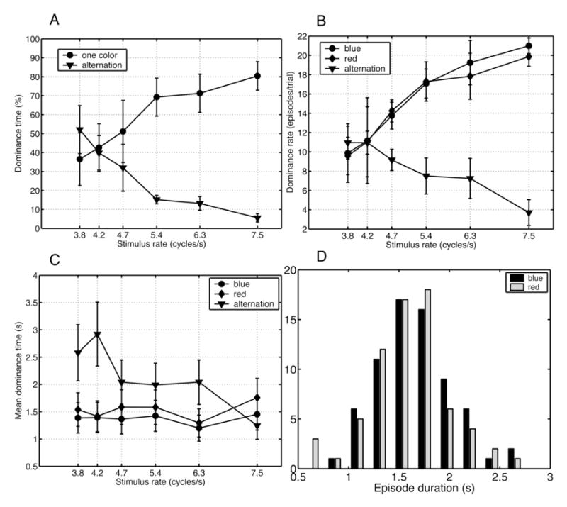
A. Shown is the fraction of total time spent experiencing a specific percept, as reported by subjects, as a function of stimulus flicker frequency(f_R). The two percepts are stable single-colored flickers (shown as circles), and alternating color flicker (shown as triangles). For each subject, reports from 4 trials at the same rate were pooled. Each point in the graph represents the mean over 6 subjects. While the total time spent experiencing red or blue flicker increases with increase in f_R, the total time experiencing alternating color flicker decreases with increase in f_R.

B. Shown are the means of reported percept durations as a function of stimulus flicker frequency. Although mean durations of single-colored flickers do not significantly change with f_R (at least not in this range of f_R), mean durations of stable alternating colored flicker are much longer at slow stimulus flicker frequency.

C. Total duration of percepts shown in A is the sum of durations of all reported episodes. This figure shows the number of reported episodes per trial, regardless of their durations, as a function of stimulus repetition rate. It differentiates between dominant red-flicker, blue-flicker, and alternating colored flicker percepts, as shown by three curves. Each point is the average over 6 subjects. Dominance rates of red and blue flickers are comparable, and increase with stimulus presentation rate. Dominance rate of alternating color flicker decreases as f_R increases.

D. Shown are the histograms of reported red/blue flicker episode durations. These values were obtained from one subject (S2), for all trials at f_R = 5.4Hz. Two distributions resemble each other in shape and values. Histograms of episode durations for other subjects and stimulus rates were similar.

Figure 2B shows that the mean dominance time, i.e., the mean duration of a reported episode of rivalry (perceiving only red or blue flicker), is around 1.4 secs, which is similar over the range of flicker frequencies used in this experiment. Thus, the increase in the proportion of time that the subject experiences rivalry between streaming flickers (red flicker and blue flicker) as flicker frequency increases is due to increase in the number of reported episodes, as shown by the dominance rate in Figure 2C. The dominance rate and mean duration of episodes of perceived alternating color flicker both decreased as the stimulus rate increased. Apparently, the number of reports of rivalry between single-color flickers increases at faster stimulus repetition rates over the range of flicker frequencies (f_R) examined. At slow rates, subjects’ reported more periods of alternating color flicker percepts each of longer duration. All subjects reported very few episodes of alternating color flicker at the faster flicker frequencies.

Figure 2D shows a histogram of dominance durations of reported episodes of blue and red flicker for one subject, for a single stimulus rate of 7.5Hz. The distributions of dominant episode durations were similar for red flicker and blue flicker percepts. All of the subjects exhibited similar distributions to the example shown, although with different mean durations (overall mean = 1.4 s). For each subject, the distributions were similar at the faster (f_R = 5.4, 6.3, and 7.5 Hz) flicker frequencies (f_R) used in this experiment. At slower frequencies (f_R = 3.7 and 4.2 Hz), the number of episodes of single-color flicker was greatly reduced, leading to greater variability in the estimates of the distribution of durations.

For all subjects, MEG data were contrasted between red flicker and blue flicker reports at the faster flicker frequencies (f_R = 5.4, 6.3, and 7.5 Hz). Because of the limited number of episodes of rivalry MEG data for the two slower flicker frequencies (f_R = 3.7 and 4.2 Hz) were not contrasted further between perceptual reports. The response at f_R = 4.7 Hz could only be contrasted in 4 of 6 subjects; the other two subjects reported only a few episodes of single-color (red or blue) flicker percepts. For these 4 subjects similar durations of red, blue, and alternating color flicker were reported at flicker frequency f_R = 4.7 Hz. The other two subjects reported similar durations of red, blue, and alternating color flicker at f_R = 5.4 Hz. For each subject, one of these two flicker frequencies was used to contrast single-color and alternating-color percepts, since all three percepts were found in comparable amounts at a single flicker frequency.

Steady-state MEG responses

The power spectrum of each 100 s trial showed a clear response at the stimulus flicker frequency (f_R) at many MEG channels. Figure 3A shows power spectra from a single trial with orthogonal red and blue flickers presented one to each eye at f_R = 4.7 Hz. In all three spectra, a peak is visible at f_R = 4.7 Hz in comparison to the background spectrum at adjacent frequencies. A robust peak is visible in each channel at 2f_R, and smaller peaks at higher harmonics, 3f_R, 4f_R, and 5f_R are visible in one channel (labeled by a green circle). We expressed the signal strength at the flicker frequency and harmonics in terms of signal to noise ratio (SNR). Topographic maps of the SNR are shown in Figure 3B at f_R, 2f_R, 3f_R, and 4f_R, averaged over the 4 trials with stimuli flickered at f_R = 4.7 Hz. The location of each channel whose spectrum is shown in Figure 3A is indicated by the corresponding circle on each map. For convenience in identifying regions we have labeled the sensor array by indicating the approximate positions of some 10-20 EEG electrodes, which indicate the major lobes of the brain (Srinivasan et al., 1999). At all flicker frequencies (and in all subjects), areas with the highest SNR at f_R were located in the posterior areas of the brain over occipital and parietal cortex. Lower SNR was observed at frontal channels with corresponding smaller peaks, as shown in Fig. 3A (magenta channel). In each subject, responses at 3f_R, 4f_R and even 5f_R were detected, although SNR at these higher harmonics were much smaller than at f_R or 2f_R.

Figure 3. Steady-state MEG responses.

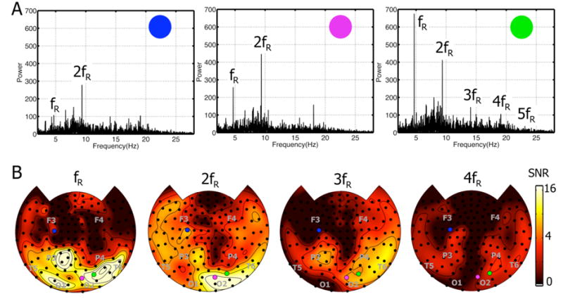
A: Power spectra of MEG responses at many channels have peaks at the flicker frequency (f_R) and its first harmonic (2f_R). Data in this figure comes from one subject (S1), from a single trial with two flickers presented out-of-phase to the two eyes at f_R = 4.7 Hz. Three representative power spectra are individually shown and the channels are labeled with colors that are used to indicate their position in part B. Only the channel on the right shows responses at higher harmonics (3f_R, 4f_R, and 5f_R). The approximate location of some 10–20 EEG electrodes are indicated by gray lettering.

B: Topographic maps of signal-to-noise ratio SNR for the fundamental (f_R) and three harmonics (2f_R, 3f_R, and 4f_R), for the same subject (S1) and flicker frequency as part A. SNR was calculated as described in the text, by dividing the power at the stimulus frequency to the power in the surrounding band. SNR maps were averaged over 4 trials counterbalancing stimulus to eye mappings. The three channels shown in part A are indicated on the maps by corresponding colored circles. The approximate location of some 10–20 EEG electrodes are indicated by gray lettering.

Control Experiments

The steady-state response at the stimulus flicker frequency (f_R) reflects activity of neurons that respond within a narrow frequency band surrounding the stimulus frequency. Figure 4A shows topographic maps of SNR at f_R = 4.7 Hz and 2f_R = 9.4 Hz for the monocular stimulation control experiment in the same subject whose rivalry trial are shown in Figure 3. In this experiment there is only one stimulus presented to one eye on each of 8 trials. SNR is much lower at both f_R and 2f_R in this experiment than in the rivalry experiment, possibly because of the passive nature of the task. At almost all sensors the response at f_R was larger than at 2f_R. In rivalry trials, responses were higher at f_R than 2f_R mainly at parietal sensors and at a few occipital sensors while responses were higher at 2f_R at frontal, temporal, and some occipital sensors, as shown by the example in Fig. 3.

Figure 4. SNR estimates for control experiments.

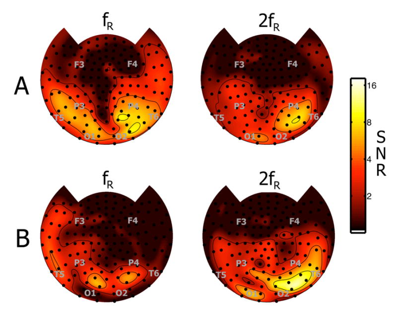
A: Monocular stimulation control. SNR maps at f_R and 2f_R are the average of 8 trials corresponding to each stimulus flicker being presented once to each eye for 60s. SNR is presented for the fundamental and second harmonic. The flicker frequency (f_R = 4.7 Hz) and subject (S1) are the same as Figure 3. The approximate location of some 10–20 EEG electrodes are indicated by gray lettering.

B. Binocular congruent stimulation control. SNR maps at f_R and 2f_R are the average of 4 trials corresponding to one stimulus flicker presented out-of-phase to each eye with the same orientation but different color. The subjects did not report rivalry. The flicker frequency (f_R = 4.7 Hz) and subject (S1) are the same as Figure 3. The approximate location of some 10–20 EEG electrodes are indicated by gray lettering.

In the rivalry experiment the two flickers are presented out of phase, one to each eye, at flicker frequency f_R. Each flicker is expected to elicit steady-state responses at f_R that are also 180 degrees out of phase. The steady-state response at one MEG sensor is the sum of activities of populations that respond to each flicker. If these responses to each flicker generate magnetic fields with radial components of equal magnitude at the MEG gradiometer coils, measured power at f_R will be zero. Thus, the magnitude of the MEG response at the stimulus flicker frequencies (f_R) is expected to reflect only the preferential sensitivity of the MEG sensor to neurons that respond to one stimulus flicker.

Figure 4B shows topographic maps for the binocular congruent stimulation control experiment. In this experiment two flickers of the same orientation but different colors are presented 180 degrees out of phase to each eye. The subjects did not report rivalry under these conditions, only a change in the perceived color of a flickering grating, from alternating red and blue at f_R = 3.5 Hz to purple at f_R = 7.0 Hz. In this control experiment we found much stronger responses at 2f_R than f_R at most sensors. When two flickers are presented 180 degrees out of phase, MEG gradiometers picking up neural signal components evoked by both eyes (each at f_R) is expected to show signals at 2f_R. Although it is possible that the two flickers evoke responses in a single (binocular) neural population at 2f_R, it is only necessary that the MEG sensor detect populations responding to each flicker.

In each example channel for a rivalry trial in Figure 3A there is a response at 2f_R, which can be larger or smaller than the response on f_R depending on sensor location. Nonlinear effects in the steady-state responses such as harmonics (Regan 1989; Srinivasan, Russell et al. 1999) are common in steady-state recordings. As shown in Figure 4A, even with monocular stimulation at f_R, there is a comparable response at 2f_R due to harmonic components of the square-wave stimulus flicker and possible nonlinear components of the flicker response. The binocular congruent stimulation control experiment indicates that if congruent stimuli were flickered out of phase to each eye, the response at 2f_R is larger than f_R. Thus, the response at 2f_R is likely to be a mixture of responses of harmonics of the responses to one flicker and responses to both flickers.

The interpretation of responses at higher harmonics (3f_R, 4f_R, 5f_R, etc.) is similarly ambiguous, since they may reflect activities of neurons that respond to both stimulus flickers, but they can also reflect harmonic responses of neurons to one stimulus flicker, which have been observed in many EEG and MEG studies (Regan 1989; Srinivasan, Russell et al. 1999; Pei, Pettet MW et al. 2002). Because of this ambiguity, we did not consider harmonics further in our analysis.

Phase and SNR analysis: rivalry versus alternation

The magnitude of the peak in the high-resolution FFT estimate (for example, Figure 3A) depends on the relative magnitude of the responses to each of the rival red and blue flickers. If the relative magnitude of these responses is sufficiently modulated by conscious perception, we anticipate the MEG sensor will exhibit 180° changes in phase between red flicker and blue flicker dominant episodes. On the other hand, MEG responses that exhibit no change in phase as the percept changes are presumably always responding preferentially to only one of the rival flickers. In this case, modulation by conscious perception is relatively weak as compared to the preference for only one physical stimulus (red or blue flicker).

We examined both phase and SNR during each perceptual report at the flicker frequency (f_R) where the subject produce similar durations of red flicker, blue flicker, and alternating color flicker reports. This frequency was 4.7 Hz is 4 subjects and 5.4 Hz in the other 2 subjects. Figure 5 shows the phase of the response at the stimulus flicker frequency (f_R = 4.7 Hz) during rivalry episodes of the same subject as Figure 3. Each row in the figure corresponds to a different perceptual report: red flicker, blue flicker, and alternating color flicker. In order to represent phase in a topographic map, we plot both cosine phase (left column) and sine phase (middle column). The extreme values in the cosine phase map correspond to 0 (+1) and 180 (−1) degrees, while the extreme values in the sine phase map correspond to 90 (+1) and 270 (−1) degrees. On each map in Figure 5, orange and magenta circles indicate channels with significant 180+/−45 degrees and 0+/−45 degrees phase differences respectively. The polar plots in the right column show both the phase and SNR (represented by radius) of each significant channel using the same color labels.

Figure 5.

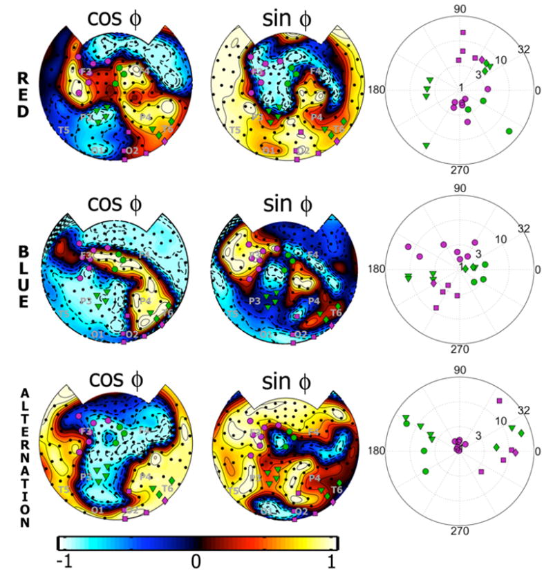
Phase and SNR for rivalry (red flicker or blue flicker perception) and alternating color flicker perception. The data shown are the phase and SNR of the response during each perceptual report for the same subject (S1) and flicker rate (fR = 4.7 Hz) as Figs. 3 and 4. SNR is calculated here separately for each perceptual report as explained in the text. Each row of plots corresponds to a different perceptual report: red flicker, blue flicker, and alternating color flicker perception. Left column: Shows topographic maps of the cosine of the phase of the cycle-averaged Fourier coefficients for each report. On each map channels that show 0 phase difference between red and blue flicker percepts are labeled in green. Channels labeled in magenta exhibit 180 +/− 45 degrees phase changes between red and blue flicker perception, corresponding to the phase difference between the flickers. The approximate location of some 10–20 EEG electrodes are indicated by gray lettering. Middle column: Shows corresponding topographic maps of the sine of phase of the cycle-averaged Fourier coefficients for each report. Right column: Polar plots of the SNR and phase of each channel showing significant 180 or 0 phase differences. SNR is represented by the radius (on a logarithmic scale). The color coding matches the topographic plots.

At any flicker frequency the phase of the response was distributed between 0 and 360 degrees across the sensors. For this subject, in the cosine phase diagrams (left column) we see that many sensors (indicated by green circles) at parietal and occipital areas of the two hemispheres remain fixed at phases near 0 (yellow areas of the map) and 180 degrees (blue areas) during both red flicker and blue flicker dominant episodes. Seven of these electrodes reached statistical significance for no phase difference. In the sine phase diagrams (middle column) we see that other occipital sensors are at phase 90 degrees (yellow areas) during red flicker perception and at phase 270 (blue areas) degrees during blue flicker perception. Five occipital sensors (magenta circles) exhibited significant 180 degrees phase changes (magenta circles). Frontal channels were also modulated following the reported percept. Seven of these sensors reached statistical significant for 180 degrees phase difference while three sensors reached statistical significance for no phase difference. Thus, at some sensors over frontal and occipital areas, the phase of the response changes as the percept changes by 180 degrees, while at other channels, mainly parietal, the phase of the response remains constant as the percept changes. This general pattern was found across all subjects at the three faster stimulation frequencies (f_R = 5.4, 6.3, and 7.5 Hz)

The interpretation of phase must be carried out with some caution, since a value of phase can be calculated even when the magnitude (or more precisely SNR) is extremely low. In this case, the phase estimate is dominated by spontaneous MEG phase. This is particularly a concern at frontal channels. Comparing the phase maps in Figure 5 to the SNR map in Figure 3B, we find that many frontal channels with significant 180 degree phase differences have low SNR in the high-resolution FFT estimate, which is averaged over all cycles of each perceptual report. This is not surprising, since responses exhibiting 180 degrees phase differences between red and blue flicker perception will cancel in the average over all cycles. To investigate the relationship between SNR and phase we calculated SNR separately for each perceptual report.

Figure 5 (right column) shows polar plots of phase and SNR for each of the channels that exhibited significant 0 or 180 degree phase shifts in the right column (using identical color coding as the phase maps in the left and middle columns). SNR estimate is represented in the radial position of the dots; the center of the plot corresponds to signal power equal to noise power (SNR = 1). In this subject, seven frontal sensors exhibited significant 180 degrees phase shifts between red flicker and blue flicker perception had smaller SNR than five occipital channels that exhibited 180 degrees phase shifts. For these seven frontal sensors, SNR ranged from 2–6 during both red and blue flicker perception. During alternating color flicker perception SNR falls below 1.5 at many of these sensors, as shown by the 7 sensors clustered at the center of the polar plot. The five occipital sensors exhibiting 180 degrees phase shifts have SNR > 3 during all three flicker percepts. Channels that exhibit no phase difference between red and blue flicker perception have SNR > 3 in all perceptual conditions, although (only for this subject and flicker frequency) SNR appears somewhat reduced during blue flicker perception at many of these sensors.

In every subject the closest balance in duration of perceptual states (in terms of red flicker, blue flicker, and alternating color flicker reports) was obtained at f_R = 4.7 Hz (4 subjects) or 5.4 Hz (2 subjects). At these frequencies, sensors that exhibit 180 degree phase shifts between red flicker and blue flicker perception were observed over the frontal lobes in each subject. Across subjects, 5–17 frontal channels reached significance for the 180 degree phase difference. The general pattern (exemplified in Figure 5) of reduced SNR during alternating color flicker perception at frontal channels that exhibit 180 degree phase shifts was also observed in each subject. However, this effect reached statistical significance in only 3 of 6 subjects. For each subject the median SNR for red flicker, blue flicker, and alternating color flicker perception was calculated across the channels exhibiting 180 degree phase shifts. Across subjects the average median SNR was 3.7; for alternating color flicker perception the average median SNR was 1.7. By contrast, occipital sensors that exhibited the 180 degree phase difference between red flicker and blue flicker perception showed robust SNR in all three flicker percept conditions (SNR = 3–30).

In every subject channels than exhibit 0 degree phase shift were mainly parietal and occipital sensors that showed robust SNR in all perceptual conditions. There was a significant reduction in SNR during the either periods of red flicker periods of blue flicker perception as compared to alternating color flicker perception at some of these channels. Differences in SNR between red-flicker and blue-flicker perception rarely reached significance, and were largest at a different set of sensors (mainly occipital and temporal) than sensors exhibiting 0 or 180 degree phase shifts.

Summary of phase results

We applied the phase analysis to all the trials at flicker frequencies (f_R = 5.4, 6.3, and 7.5 Hz) with enough red flicker and blue flicker reports to conduct the statistical analysis in each subject. Figure 6 shows averaged phase difference patterns obtained for each subject by calculating the phase difference at each flicker frequency and then averaging over flicker frequencies. Although not exactly overlapping, robust phase differences of 180 degrees (cos Df = −1) are observed in each subject at midline frontal sensors and no phase difference (cos Df = +1) are observed at parietal and parietal/occipital sensors across the subjects. Channels that reached significance in at least 2 of 3 flicker frequencies are indicated by green (no phase difference) and magenta (180 degree phase difference) circles. A general differentiation between parietal cortex (no phase shift) and frontal cortex (180 degree phase shift) was observed in all subjects. There were, of course, exceptions at specific frequencies and stimulus-to-eye mappings as shown in Figure 5 where some frontal channels exhibit 0 phase differences. In every subject, almost no sensors were found that exhibited significant intermediate phase differences (close to + or − 90 degree).

Figure 6.

Summary of phase difference between red-flicker and blue-flicker perception averaged across faster flicker frequencies (f_R = 5.4, 6.3 and 7.5 Hz). For each subject, topographic maps are the cosine of the phase difference between the cycle-averaged Fourier coefficients for red flicker perception and blue flicker perception. The phase difference was averaged over the three flicker frequencies. On each map channels that show 0 +/− 45 degrees phase difference between red and blue flicker percepts for at least 2 of 3 flicker frequencies are labeled in green. Channels labeled in magenta exhibit 180 +/− 45 degrees phase changes between red and blue flicker perception for at least 2 of 3 flicker frequencies. The approximate location of some 10–20 EEG electrodes are indicated by gray lettering.

The sensors that exhibited close to 180°(+/− 45 degrees) phase changes were primarily sensors located over frontal areas, and some occipital and occipital/temporal sensors. The precise location of these sensors varied between subjects, but in every subject, some midline frontal sensors exhibited 180° phase differences. The response of occipital channels depended more on the subject, flicker frequency, and stimulus to eye mapping. The data shown for one subject in Figures 4 and 5 was collapsed over 4 different trials at the same stimulus flicker frequency (f_R = 5.4 Hz). These trials presented each stimulus feature combination of orientation (horizontal or vertical) and color (red or blue), once to each eye (with the other combination presented to the other eye). The data were averaged to emphasize effects that were independent of stimulus configuration. We confirmed that 180° phase shifts in the MEG that follow shifts in perception between the red and blue flickers were found within individual trials, each with a specific stimulus configuration. On a trial-by-trial basis, we consistently found that the effects at anterior sensors were relatively independent of stimulus configuration, and easily observed in the averaged analysis. Furthermore, stronger phase difference effects were found at posterior sensors in single trials than in the averaged data, indicating that responses over posterior areas showed greater dependence on the specific stimulus to eye mapping, which made these phase shifts less readily observed in the averaged analysis. We did not further explore the details of these stimulus feature specific effects at posterior sensors, as these were also highly variable across subjects.

Synchronous Rivalry Control Experiment

A synchronous rivalry control condition was run on one subject, where the red and blue flickers were presented simultaneously at flicker frequency 5.4 Hz. In this display, the red and blue images were presented on the same video frames and there was no phase difference between the flickers presented to each eye. The subject reported rivalry, with similar behavioral results as out of phase presentation given in Figure 2. Analysis of phase differences between red flicker and blue flicker dominant episodes revealed that only zero phase differences were statistically significant. Thus, the 180 degree phase shifts we observe with out of phase stimulus flicker appears to be related to the physical stimulation with 180 degree phase differences.

Discussion

Rivalry between flickers

In this experiment, we investigated a form of binocular rivalry between two images that are flickered one to each eye, but are never presented simultaneously to the observer. The images are presented in alternation, with brief dark intervals (60–130 ms) between images. Despite the alternation, the subjects spontaneously experienced the stimuli either as alternating images (one unitary flicker composed of both images), or as two separate single-image flickers that appeared to rival in the manner of conventional rivalry. The amount of reported rivalry appears to depend on the flicker frequency over the range of 3.5 – 7.5 Hz, replicating the results of O’Shea and Crassini (1984). The duration of an episode of perceptual dominance of one flicker was very similar at all flicker frequencies for each subject. At slower flicker frequencies the number of reported episodes of rivalry decreases. At the same time, both the number and duration of alternating color flicker percepts increases with decreasing flicker frequency.

Although each image is presented briefly (13 ms) to each eye, followed by a longer dark interval, the responses of LGN cells decay slowly, over a period as long as 300 ms when no masking stimulus is presented (Keysers and Perrett, 2002; Rolls and Tovee, 1994). The duration of persistent response in cells in the cortex (e.g., inferior temporal cortex) can also be as long as 300 ms. Hence, even when there is no simultaneous physical stimulation for each eye, when the stimulus is presented to one eye there are still likely to be weak inputs to primary visual cortex from LGN in response to the last image presentation in the other eye. Moreover, persistent responses will also be found in reentrant cortical networks that functionally couple visual cortex to other cortical areas, and appear to respond for as long as 300 ms after stimulus presentation. The number of episodes of rivalry between single-image flickers decreases as the temporal frequency decreases below 5 Hz and becomes negligible below 3 Hz (Oshea and Crassini, 1984). This lower limit corresponds to a stimulus repeating every 333 ms in one eye or an interval of 167 ms between presentations to each eye.

We suggest that the interval between presentations of a stimulus into one eye determines the perceptual organization of the sequence of stimuli either into two separate single-color flickers or one alternating color flicker. The ‘critical Gestalt fusion frequency’ in the context of a single (binocular) flickering stimulus (van de Grind et al., 1973) exhibits a similar limit of around 3 Hz. Above this threshold frequency, spatial structure of a flickering pattern reaches persistence, and does not completely disappear during dark periods. Reported values of Gestalt fusion frequencies are between 3.5–4.5 Hz, and are robust to the binocular presentation of a distracting flicker. Similarly, in the present experiment the alternated stimuli are perceived as single-color flickers that rival at 5.4 Hz and higher frequencies in every subject.

The process of analyzing the temporal structure of the stimuli, in order to “group” together stimuli that are from the same source (stimulus x eye) into a single-color flicker apparently has an upper limit of around 300 ms. Perceptual grouping may play an important role in the change of percept from alternating color flicker to rivalry between single-color flickers experienced by our subjects as flicker frequency increases. In auditory perception, this process has been termed stream segregation (Bregman, 1990), and by analogy we refer to it as visual stream segregation. In visual stream segregation, subjects can perceptually group a repeating visual stimulus into a flicker, despite the intermediate presentation of an incongruent rival stimulus to the other eye. In auditory streaming experiments where interstimulus interval, repetition interval, and stimulus duration were varied separately, the difficulty in streaming the stimuli depended on the repetition interval of a stimulus, rather than the interstimulus interval (Bregman, Ahad et al. 2000). In auditory streaming, the upper limit for the repetition interval is around 200 ms, similar to visual streaming in the present experiment. This suggests that streaming the stimuli into distinct flickers is critical to rivalry between flickers reported here.

An alternative hypothesis is that rivalry takes place between pairs of images, even if they are not presented simultaneously, when the interstimulus interval is less than 100 ms. A limit of 100 ms for binocular interactions has been demonstrated for binocular (luminance) summation with flickering stimuli (Thorn and Boynton 1974), stereopsis (Dodwell and Engel 1963), and during rivalry both in the study by O’Shea and Crassini (1984), and in the present study. In both rivalry studies, interval between repetitions of the same stimulus was fixed, and it was always twice the interstimulus interval, and they were not investigated independently. However, we note that when f_R = 3.33 Hz the subject does not experience rivalry although the interstimulus interval is only 150 ms, indicating that the responses to the two incongruent stimuli (which can persist for 300 ms) are present in the visual system. On the other hand, the responses to repetition of the same stimulus are separated by more than 300 ms, possibly restricting the perceptual grouping of the repeating stimulus into a flicker. Further experiments that consider presentations of the two visual flickers at different phase differences (similar to the auditory experiment) are still necessary to clarify whether effect depends on the interstimulus interval, or the flicker frequency alone.

MEG phase at frontal sensors follows conscious perception

Steady-state responses were observed in a narrow band (Df = 0.01 Hz) at the frequency of stimulus flicker to each eye at many MEG sensors. We interpret this steady-state MEG response as reflecting the preferential sensitivity of the sensors to populations that respond synchronously to one of the flickers. MEG sensors that record from two neural populations (or even just one population) that each respond equally to both flickers will generate responses at the flicker frequency that are 180 degrees out of phase and hence cancel. Since our subjects experienced rivalry between two physical flickers at the same frequency, but presented out of phase, we hypothesized that if the dominant response detected by an MEG sensor switches following conscious perception, we should observe changes in phase between episodes of perceiving one flicker, and episodes of perceiving the other flicker. Phase modulation following changes in conscious percept was observed in every subject at each flicker rate that induced rivalry, over frontal and occipital cortex. Frontal phase modulations were robust with respect to stimulus configuration factors, such as grating orientation to color mapping or eye to stimulus color mapping. Occipital phase modulations appeared to be more dependent on the specific mapping of stimulus configuration to eye.

We found a distributed network encompassing anterior and posterior brain regions that synchronizes to the perceived flicker during rivalry. An earlier result implied that a correlate of sustained conscious percept of one flickering image to be increased synchronization between occipital and frontal areas of the brain, at the corresponding stimulus flicker frequency (Srinivasan, Russell et al. 1999). In that experiment, two images were flickering at distinct frequencies, eliciting responses with different distributions over the array of MEG sensors. We were not able to easily observe synchronization/desynchronization of responses at the pair of frequencies in relation to conscious perception at a single sensor location. In this study, we have used a single flicker frequency presented out-of-phase to the two eyes, and we find evidence that both anterior and posterior sensors become phase-locked to the perceived flicker. Due to the limited (cm scale) spatial resolution of MEG (Hamalainen, Hari et al. 1993; Srinivasan, Russell et al. 1999), we cannot be more specific about the cortical areas that are involved in this anterior-posterior network.

MEG phase at parietal sensors indicates dominance of one flicker

By contrast to occipital and frontal sensors, sensors over parietal areas with robust steady state responses showed no phase modulation during rivalry. MEG sensors over parietal cortex detect response components of neural populations that are preferentially responding to one of the flickers irrespective of which flicker is perceived. This provides a partial explanation of why the high-resolution FFT estimate of the steady-state responses at the stimulus rate was much lower at sensors over frontal areas as compared to parietal sensors. In frontal areas, responses during episodes of dominance of one flicker are out of phase with responses at other intervals, and they at least partially cancel out. Very little signal is observed at these sensors in the average SNR over all cycles (high-resolution FFT), nor separately during alternating color flicker perception. SNR was elevated during perception of either single-color flicker, but these two responses were 180 degrees out of phase. Signals over parietal areas show the least amount of phase variation, and hence the highest steady-state responses (and signal to noise ratios) at the stimulus flicker frequency. These parietal responses appear relatively weakly modulated by conscious perception.

Rivalry in reentrant networks spanning thalamus to frontal cortex

Where and how rivalry takes place is a controversial issue. Evidence exists to support both early (eye) and late (form) aspects of competition leading to rivalry (Blake and Logothetis 2002). In the present experiment competition between rival flickers potentially takes place due to interocular competition between successive stimuli in early stages of visual information processing, due to likely persistence of responses to each stimulus presentation on the order of 300 ms. Thus, competition could still take place between the eyes, close to the input stage in primary visual cortex, even though the stimuli are not presented simultaneously. However, if this were the most important contribution to rivalry, we might expect robust rivalry at a flicker rate of 3.33 Hz, since the two out-of-phase flickers are separated by only 150 ms. Neither in this study nor in the original study of Oshea and Crassini (1984) was much rivalry reported below 4 Hz. We propose that the rivalry in this experiment takes place between the flickers, rather than individual images. This scenario is consistent with the notion rivalry occurs between higher-level stimulus representations (Leopold and Logothetis 1999) that involve areas beyond visual feature processing, such as inferior temporal and frontal areas. It is well-known that neural activity related to visual information processing depends on both thalamo-cortical networks and corticocortical reentrant connections that dynamically couple distant cortical areas both within, and outside the visual system (Felleman and Van Essen 1991; Tononi, Sporns O. et al. 1992). Reentry involves interactions between very distant cortical areas, which suggests that propagation times between cortical areas constrain the network dynamics. Propagation delays in long-range corticocortical fibers connecting anterior and posterior regions are estimated in the 50–100 ms range (Nunez, 1995). Thus, the time period where stimulus-related neural responses appear throughout visually driven large-scale cortical networks may be on the order of 200–300 ms consistent with intracranial recordings of local field potentials in animal models with electrodes distributed over the cortex (Bressler, 1995), and the known persistence of responses in single-unit recordings (Keysers and Perrett, 2002; Rolls and Tovee, 1994). Thus, when flicker rate exceeds 5 Hz, perceptual grouping of a single image flicker may be facilitated by the persistence of neural responses to the same stimulus in large-scale cortical networks. This would be consistent with the idea that the competition is between forms (incongruent flickers) represented in the total activity in a distributed cortical network (Mountastle, 1997). Increased synchronization in relation to conscious perception has been observed in such a distributed network involving sensors over frontal and occipital areas both in the present study and in a previous study using two asynchronous flickers (Srinivasan et al., 1999).

Conclusions

In this study we have demonstrated a form of rivalry that emerges from the perceptual organization of a stream of incongruent stimuli, presented alternately one to each eye, into two incongruent flickers. For this grouping to occur reliably, each stimulus should be repeated in one eye within 200 ms. If the two images are perceptually grouped into two flickers, they rival in the manner of conventional rivalry, and the subject reports episodes of perceiving only one flicker. A cortical network including populations of frontal and occipital sensors appears to synchronize to the perceived flicker during these episodes, consistent with our previous MEG and EEG studies with asynchronous flickers (Srinivasan et al., 1999; Srinivasan, 2004). This network is apparently sensitive to temporal properties of stimulus driving the conscious percept.

References

- Blake Fox, et al. Stochastic properties of stabilized-image binocular rivalry alternations. Journal of Experimental Psychology. 1971;1971:327–332. doi: 10.1037/h0030877. [DOI] [PubMed] [Google Scholar]
- Blake R, Logothetis N. Visual competition. Nature Reviews Neuroscience. 2002;3:13–21. doi: 10.1038/nrn701. [DOI] [PubMed] [Google Scholar]
- Brainard DH. The Psychophysics Toolbox. Spatial Vision. 1997;10:433–436. [PubMed] [Google Scholar]
- Bregman Auditory Scene Analysis 1990 [Google Scholar]
- Bregman A, Ahad P, et al. Effects of time intervals and tone durations on auditory stream segregation. Perception & Psychophysics. 2000;62(3):626–636. doi: 10.3758/bf03212114. [DOI] [PubMed] [Google Scholar]
- Bressler SL. Large-scale cortical networks and cognition. Brain Research Reviews. 1995;20:288–304. doi: 10.1016/0165-0173(94)00016-i. 1995. [DOI] [PubMed] [Google Scholar]
- Dodwell P, Engel G. A theory of binocular fusion. Nature. 1963;198(39–40) doi: 10.1038/198039a0. [DOI] [PubMed] [Google Scholar]
- Fahle Binocular Rivalry: Suppression Depends on Orientation and Spatial Frequency. Vision Res. 1982;22:787–800. doi: 10.1016/0042-6989(82)90010-4. [DOI] [PubMed] [Google Scholar]
- Felleman D, Van Essen D. Distributed hierarchical processing in the primate cerebral cortex. Cereb Cortex. 1991;1:1–47. doi: 10.1093/cercor/1.1.1-a. [DOI] [PubMed] [Google Scholar]
- Fox, Herrmann Stochastic properties of binocular rivalry alternations. Perception&Psychophysics. 1967;1967:432–436. [Google Scholar]
- Fries P, Roelfsema P, et al. Synchronization of scillatory responses in visual cortex correlates with perception in interocular rivalry. Proc Natl Acad Sci USA. 1997;94:12699–12704. doi: 10.1073/pnas.94.23.12699. [DOI] [PMC free article] [PubMed] [Google Scholar]
- Hamalainen M, Hari R, et al. Magnetoencephalography-theory, instrumentation, and applications to noninvasive studies of the working human brain. Rev Mod Phys. 1993;65:413–497. [Google Scholar]
- Keysers C, Perrett DI. Visual masking and RSVP reveal neural competition. Trends in Cognitive Sciences. 2002;6:120–125. doi: 10.1016/s1364-6613(00)01852-0. [DOI] [PubMed] [Google Scholar]
- Leopold D, Logothetis N. Activity changes in early visual cortex reflect monkeys’ percepts during binocular rivalry. Nature. 1996;379:549–553. doi: 10.1038/379549a0. [DOI] [PubMed] [Google Scholar]
- Leopold D, Logothetis N. Multistable phenomena: changing views in perception. Trends in Cognitive Sciences. 1999;3(7):254–264. doi: 10.1016/s1364-6613(99)01332-7. [DOI] [PubMed] [Google Scholar]
- Levelt The alternation process in binocular rivalry. British Journal of Psychology. 1967;58:143–145. doi: 10.1111/j.2044-8295.1967.tb01068.x. [DOI] [PubMed] [Google Scholar]
- Lumer E, Rees G. Covariation of activity in visual and prefrontal cortex associated with subjective visual perception. Proc Natl Acad Sci USA. 1999;96:1669–1673. doi: 10.1073/pnas.96.4.1669. [DOI] [PMC free article] [PubMed] [Google Scholar]
- Mueller T, Blake R. A Fresh Look at the Temporal Dynamics of Binocular Rivalry. Biological Cybernetics. 1989;61:223–232. doi: 10.1007/BF00198769. [DOI] [PubMed] [Google Scholar]
- O’Shea R, Crassini B. Binocular rivalry occurs without simultaneous presentation of rival stimuli. Perception & Psychophysics. 1984;36(3):266–276. doi: 10.3758/bf03206368. [DOI] [PubMed] [Google Scholar]
- Pei F, Pettet MW, et al. Neural correlates of object-based attention. J Vis. 2002;2(9):588–96. doi: 10.1167/2.9.1. [DOI] [PubMed] [Google Scholar]
- Pelli DG. The VideoToolbox software for visual psychophysics: Transforming numbers into movies. Spatial Vision. 1997;10:437–442. [PubMed] [Google Scholar]
- Regan D. Human brain electrophysiology 1989 [Google Scholar]
- Rolls ET, Tovee MJ. Processing speed in the cerebral cortex and the neurophysiology of visual masking. Proc R Soc London B Biol Sci. 1994;257:9–15. doi: 10.1098/rspb.1994.0087. [DOI] [PubMed] [Google Scholar]
- Silberstein R. Steady-state visually evoked potentials, brain resonances, and cognitive processes. In: Nunez PL, editor. Neocortical Dynamics and Human EEG. 1995. [Google Scholar]
- Srinivasan R. Internal and external neural synchronization during conscious perception. The International Journal of Bifurcation and Chaos. 2004 doi: 10.1142/S0218127404009399. [DOI] [PMC free article] [PubMed] [Google Scholar]
- Srinivasan R, Russell P, et al. Increased Synchronization of Neuromagnetic Responses during Conscious Perception. The Journal of Neuroscience. 1999;19(13):5435–5448. doi: 10.1523/JNEUROSCI.19-13-05435.1999. [DOI] [PMC free article] [PubMed] [Google Scholar]
- Thorn F, Boynton R. Human binocular summation at absolute threshold. Vision Res. 1974;14:445–458. doi: 10.1016/0042-6989(74)90033-9. [DOI] [PubMed] [Google Scholar]
- Tong F, Nakayama K, et al. Binocular rivalry and visual awareness in human extrastriate cortex. Neuron. 1998;21:753–759. doi: 10.1016/s0896-6273(00)80592-9. [DOI] [PubMed] [Google Scholar]
- Tononi G, Sporns O, et al. Reentry and the problem of integrating multiple cortical areas: simulation of dynamic integration in the visual system. Cereb Cortex. 1992;2:310–335. doi: 10.1093/cercor/2.4.310. [DOI] [PubMed] [Google Scholar]
- Wolfe J. Influence of spatial frequency, luminance, and duration on binocular rivalry and abnormal fusion of briefly presented dichoptic stimuli. Perception. 1983;12:447–456. doi: 10.1068/p120447. [DOI] [PubMed] [Google Scholar]