Volume Estimates by Imaging Methods: Model Comparisons with Visible Woman as the Reference

Abstract

Objective

To compare the accuracy of four volume estimation models to actual tissue and organ volumes measured in the visible woman.

Methods

Actual volumes were calculated from 1-mm-thick visible woman images that were segmented for five major components including subcutaneous and visceral adipose tissue across the 1730 available slices. Four available models resolved to two equations: truncated cone/truncated pyramid vs. two-column/parallel trapezium. Between-slice interval and initial slice were systematically varied when deriving component volumes using the two equations in four regions.

Results

For each compartment and each between-slice interval, the means of the two-column model were always the same as the corresponding reference volumes, whereas those of the truncated cone model were smaller than the reference volumes. Similarly, the coefficient variation for the two-column model was always smaller than for the truncated cone model.

Discussion

The equation based on the parallel trapezium and the two-column models is more accurate in estimating tissue volumes than the corresponding equation for truncated pyramid and truncated cone models. This finding has important implications for the volume calculations of imaging-based body compartments such as adipose tissue.

Introduction

Imaging methods, including computerized axial tomography (CT)1 and magnetic resonance imaging (MRI), are now applied as the reference methods for measuring whole-body and regional tissue and organ volumes in vivo (1–4). The availability of MRI and CT over the past 2 decades has improved the understanding of physiological (3) and pathological (5,6) conditions related to the size and structure of body components.

Both CT and MRI acquire axial images of known thickness, usually 5 to 10 mm. The organ or tissue of interest is next segmented within each slice to provide an area estimate. Because acquisition and analysis of contiguous MRI scans of the whole body are very time-consuming and expensive, axial images are instead collected with inter-slice gaps typically ranging from 20 to 40 mm. Volumes are then calculated using geometric models based on the measured areas and the distances between adjacent slices. There are three different models now in use (Table 1) (2,7), and their validity has not been critically tested using actual human tissues of known volume. In particular, there are no comparisons of these models across different tissues in different regions.

Table 1.

The four geometric models

Model	Geometric Shape	Volume (Vi)
Actual Shape
Truncated Pyramid		$V_i=h(A_i+A_{i+1}+\sqrt{A_i{A}_{i+1}})/3$
Truncated Cone		$V_i=h(A_i+A_{i+1}+\sqrt{A_i{A}_{i+1}})/3$
Parallel Trapezium		$V_i=h(A_i+A_{i+1})/2$
Two-Column		$V_i=h(A_i+A_{i+1})/2$

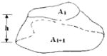
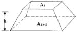
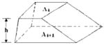
Although the tissues in axial images are always irregularly shaped, there are three reported volume models in the medical literature to estimate volumes of adjacent slices with certain between-slice intervals: truncated pyramid model (2,17), truncated cone model (4,7), and the parallel trapezium model (7). The three models all assume that the change in cross-sectional area between two adjacent scans is linear, and the irregular shapes of the tissue in an axial slice are assumed to be a square, circle, and parallel trapezium, respectively. We propose a new model: the two-column model. The geometry of the compartment of interest is assumed to be represented by two columns, both having the original shape of the tissues in cross-section and a height of one-half of the between-slice distance.

The Visible Human Project of the National Library of Medicine initiated the analysis of 1-mm-thick consecutive high-resolution axial photographs of a middle-aged man and woman (8). The availability of the Visible Human data, specifically the visible woman (VW), led us in the current study to segment the major tissues across the 1730 axial images and then to use these data as the reference against which we compared the equations of three earlier and one new volume model.

Research Methods and Procedures

VW Segmentation

The Visible Human Project acquired transverse CT, magnetic resonance, and cryosection images of representative male and female cadavers. The original cryosection images of the female cadaver are at 0.33-mm intervals, but in the present study, we analyzed the 1-mm image series that provides adequate accuracy for reference volume estimations. The 1730 axial VW photographs were analyzed by one trained observer using an in-house image segmentation software program (9,10) developed based on the Interactive Data Language environment at the New York Obesity Research Center. The software is specifically designed for imaging-based body composition research. In this study, semiautomatic segmentation methods (e.g., thresholding and region-growing) and interactive image-editing tools were employed in data analysis.

The body was divided into four sections as defined by anatomical landmarks into the head and neck, upper limbs, lower limbs, and trunk. The neck was separated from the trunk section at the upper border of the clavicle. Upper limbs were separated from the trunk at the axillary level. Lower limbs were isolated from the trunk at the ischial tuberosity. The images were segmented into five components, subcutaneous adipose tissue (SAT), visceral adipose tissue (VAT), skeletal muscle (SM), lung, and remainder. As is the practice for MRI segmentation (2,11), tissues of the head, hands, and feet were segmented as a remainder comprised of bone, organs, and connective tissues. This provided a total of 12 compartments including 3 each in the upper limbs and lower limbs (i.e., SM, SAT, and remainder), five in the trunk (i.e., SM, SAT, VAT, lung, and remainder), and the head and neck.

VW Volume Calculations

The volumes of the 12 body compartments were calculated from the 1730 VW axial photographic images and were taken as the reference volumes:

$$V_r=\sum _{i=1}^N(1\times A_i)$$ (1)

where N is the total slice number of one compartment and A_i is the cross-sectional area of each slice.

Evaluated Volume Models

In general, CT and MRI provide axial images with a known thickness and a specified between-slice interval. There are three reported volume models in the medical literature to estimate the volumes that exist between adjacent slices, and these are summarized in Table 1. The three models all assume that the change in cross-sectional area between two adjacent scans is linear and that the irregular shapes of the tissue in an axial slice are assumed to be a square, circle, and parallel trapezium, respectively. The three models are referred to as the truncated pyramid model, the truncated cone model, and the parallel trapezium model, respectively (7).

The three models assume that the shapes of tissues in axial slices are geometrically regular, whereas most human tissues are actually irregular shapes. Therefore, in the present study, we evaluated a fourth model referred to as the two-column model (Table 1). The geometry of the compartment of interest was assumed as two columns, both having the original shape of the tissues in the cross section and a height of one-half of the between-slice distance.

For both truncated pyramid and truncated cone models, the volume between two adjacent slices can be calculated with the formula:

$$V_i=h(A_i+A_{i+1}+\sqrt{A_i{A}_{i+1}})/3$$ (2)

where V_i is the volume between adjacent scans, A_i and A_i+1 are the adjacent scan areas, and h is the between-slice distance.

The two-column model formula is the same as the parallel trapezium model formula:

$$V_i=h(A_i+A_{i+1})/2$$ (3)

Thus, the four volume models resolve to two equations (i.e., Equations 2 and 3). Accordingly, for each compartment, the sum of slice volumes and all between-slice volumes estimated by Equations 2 and 3 are presented as Equations 4 and 5, respectively.

$$V_1=t\sum _{i=1}^N{A}_i+h/3\sum _{i=1}^N[A_i+A_{i+1}+\sqrt{(A_i{A}_{i+1})}]$$ (4)

$$V_2=(t+h)\sum _{i=1}^N{A}_i$$ (5)

where A_i and A_i+1 are the areas of two adjacent scans, h is the interval between adjacent sampled slices, t is the thickness of each slice, and N is the number of total slices.

The accuracy of volume estimates by Equations 4 and 5 were evaluated in the present report by comparing with the reference volume derived from the 1-mm-thick consecutive VW.

The estimated volumes of all 12 compartments were calculated with a slice thickness of 10 mm and intervals of 10, 20, 30, 40, 50, 60, 70, and 80 mm at all possible starting points. For each interval, we systematically varied the starting point by 1-mm increments. The number of possible starting points is the sum of the slice thickness and the between-slice intervals. For example, 30 possible starting points were considered for the 20-mm slice interval.

The acquired data included five components (SAT, SM, VAT, lung, and residual) in four regions (trunk, upper limbs, lower limbs, and head and neck). This provided a total of 12 estimates including 3 each in the upper limbs and lower limbs, 5 in the trunk, and the head and neck. In the analysis, we considered two volume estimation equations in comparison to the corresponding reference VW volume. For each compartment, to summarize data for each of the slice intervals, we calculated the volume mean and coefficient of variation (CV) of the volumes resulting from different starting points for each of the equations. We then compared the mean volumes derived by the two equations to the reference volume. The CVs for the two equations were also compared with each other. Our analysis approach yielded many results, although the findings were consistent across regions and components. Therefore, we provide a simplified description of the findings in the Results section. Specifically, the most common whole-body protocol involves axial images with 40-mm intervals, and we selected this interval for demonstration purposes.

All analyses were carried out using the SPSS/PC statistical program (version 9.0 for Windows; SPSS, Inc., Chicago, IL). Two-tailed (α = 0.05) tests of significance were used.

Results

VW Reference Volumes

The results of VW component reference volumes are presented in Table 2. The trunk had the largest section volume, followed by the lower limb, upper limb, and head and neck. SAT was the largest compartment in each region; trunk SAT was 37.4% of trunk volume, lower limb SAT was 45.7% of lower limb volume, and upper limb SAT was 43.4% of upper limb volume.

Table 2.

VW component reference volumes

Section component	Volume (liter)
Head and neck	5.56
Trunk	49.30
SAT	18.45
SM	10.53
VAT	4.30
Lung	2.56
Remainder	13.46
Upper limb	8.35
SAT	3.63
SM	3.28
Remainder	1.45
Lower limb	19.51
SAT	8.92
SM	7.40
Remainder	3.19
Total body	82.73

Model Comparisons

For the 40-mm slice interval, the mean of VAT calculated with Equations 4 and 5 were 4.19 and 4.30 liters, or −2.2% and 0%, respectively, from the reference value. The corresponding results for SAT of the lower limbs were 8.53 and 8.92 liters, −3.5% and 0% compared with the reference value. Upper limb muscle results showed a similar trend, 3.15 and 3.28 liters, or −2.1% and 0% compared with the reference value. The mean values for all of the other compartments calculated using Equation 5 were exactly the same as the reference volumes, whereas the means for Equation 4 were 1.3% to 6.4% smaller than the corresponding reference volumes.

The CV of VAT for Equation 4 was larger (3.5%) than that for Equation 5 (3.1%). The corresponding results for SAT were 8.0% and 7.6%, respectively. For upper limb muscle, the CV for Equation 4 was larger than for Equation 5, 3.3% vs. 1.7%. The CVs for all other compartments estimated by Equation 4 were larger (2.3% to 11.6%) than those estimated by Equation 5 (0.6% to 11.4%).

These results are graphically portrayed in Figure 1. The figure shows means and CVs for the 12 evaluated compartments organized by increasing mean difference from the reference value. Equation 5 showed no mean differences from the reference values, and these data are not presented in the figure. The mean differences for Equation 4 from the reference value range from −1.3% to −6.4%. The CVs range from 0.6% to 11.6%, with the CV for Equation 4 always larger than for Equation 5.

Figure 1.

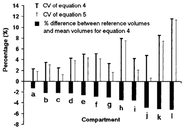
The 12-compartment results for the 40-mm slice interval. The results are organized by increasing mean volume difference between Equation 4 estimates and the corresponding reference values. The mean volume results for Equation 5 did not differ from the reference values and are not shown in the figure. The figure also provides the 12-compartment CVs for Equations 4 and 5. (a) Trunk remainder. (b) VAT. (c) Upper limb SAT. (d) Trunk SAT. (e) Lower limb SM. (f) Trunk SM. (g) Upper limb SM. (h) Lower limb SAT. (i) Lower limb remainder. (j) Lungs. (k) Upper limb remainder. (l) Head and neck.

For all the other between-slice distances, 10, 20, 30, 50, 60, 70 and 80 mm, Equation 5 always had mean values equivalent to the reference volumes. This result can be proven mathematically as shown in Appendix 1. Equation 5 also had smaller CVs than those provided by Equation 4.

Relationship between Slice Interval and Accuracy

For both equations, with an increase in slice interval, there was a trend toward increasing CVs for all compartments (p < 0.001). The relationship of slice interval and CV is presented in Figure 2. Some compartments had higher CVs at specific smaller between-slice intervals. For example, CVs for VAT and trunk SAT at various slice intervals are presented in Figure 3. For VAT, the 30-mm interval CVs for Equations 4 and 5 were 1.8% and 1.1%, respectively. These CVs are smaller than the 2.4% and 2.3% for the 20-mm interval; the 70-mm interval CVs were 4.6% and 1.9%, respectively. These CVs are smaller than the CVs of 5.9% and 4.7% for the 60-mm interval. For trunk SAT, the 70-mm interval CV for Equation 4 was 5.9%, which was smaller than the 60-mm interval CV of 6.3%.

Figure 2.

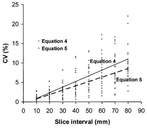
The relationship between CV and slice interval for all compartments. There are 24 points at each interval, 12 for Equation 4 and 12 for Equation 5. Corresponding regression lines for the two equations are shown in the figure.

Figure 3.

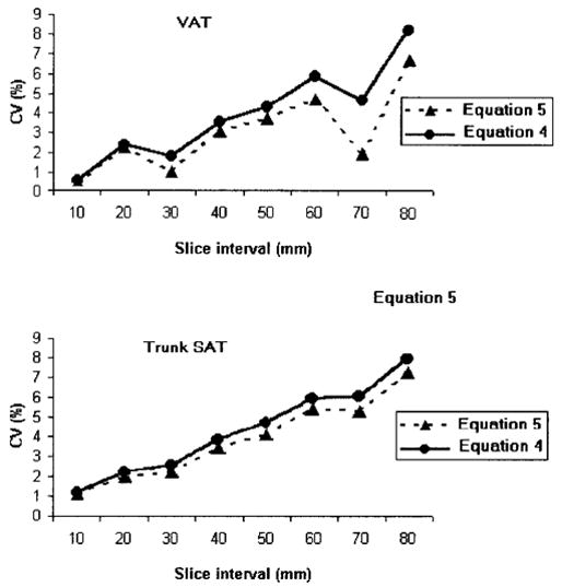
The CVs for VAT and trunk SAT at various slice intervals for Equations 4 and 5.

Discussion

Equation Accuracy

Anthropometric measurement of leg volume using a geometric model, a truncated cone, was first reported by Jones et al. in 1969 (12). In the past 2 decades, CT and MRI have greatly improved the accuracy of measured component areas and, thus, total tissue volumes. Earlier investigators focused their analysis of volume reconstruction model accuracy solely on quantification of adipose tissue (7), and the model results were not compared with “actual” tissue volumes. This is because cadaver studies are difficult to perform, and it is hard to measure accurately the regional component’s weight that corresponds exactly to the volume estimate provided by imaging methods.

Both Equations 4 (2,4,14–17) and 5 (1,6,13,18–24) were applied by earlier investigators to their CT and MRI volume calculations. Before the present investigation, the choice of reconstruction model was based largely on investigator preference rather than on experimental data. One goal of moving imaging methods toward reference method status is to establish the most accurate approach for deriving compartment volume from measured areas.

In the present study, we employed a novel approach by comparing model-derived volumes to a measure of “actual” tissue volume compiled from 1730 contiguous 1-mm-thick VW images. Unlike traditional cadaver dissection, volume and not mass of individual structures was evaluated. Thus, we were able to compare the reference volumes of the 12 compartments with the corresponding mean of volumes estimated by the two equations, and we also compared the CVs of data provided by the two equations to each other. Our main finding, based on slice intervals typically used by investigators, is that volume estimates derived using Equation 5 are consistently superior to those provided by Equation 4.

Our findings are based on only one cadaver, but the analyses included 4 regions and 12 compartments that varied greatly in their size and three-dimensional structure. Thus, we can conclude that Equation 5 is more accurate than Equation 4 in quantifying a wide range of human tissues, and Equation 5 should, accordingly, be adopted for imaging method tissue volume quantification. To our knowledge, this is the first study to evaluate volume models in several tissues distributed in different regions.

For a particular compartment, the means of Equation 4 were always smaller than the reference tissue volume, suggesting that most reference tissue volumes between adjacent slices are more convex than described by truncated cone or truncated pyramid models. This phenomenon was observed in all 4 regions and 12 compartments and with different slice intervals.

MRI is also used to quantify organ volumes. However, because organ volumes are usually derived from continuous scan protocols, the volume is actually calculated as:

$$V=t\sum _{i=1}^N{A}_i$$

Because there is no between-slice volume estimation in this calculation, the discussion of the accuracy of MRI for organ volume quantification is not relevant in the present study.

In addition to accuracy, Equation 5 also has advantages in quantifying the combined volumes of muscle, adipose tissue, and other tissues in a selected region. There are two methods available to calculate the combined volume. By using the first method, the volumes of muscle, adipose tissue, and other tissues are calculated separately by an equation and then summed to yield the combined volume “V₁”. With the second method, the areas of muscle, adipose tissue, and other tissues in each slice are summed to obtain the total area and the total volume (“V₂”) is then calculated using an equation. According to our calculation in Appendix 2, V₁ is always equal to V₂ for Equation 5, and V₁ is always smaller than V₂ for Equation 4. Because most reports do not state the detailed calculation steps, inconsistency may occur when different calculation methods are adopted. Although the percentage error might be small, investigators and readers might be confused if the sum of the region volume is not equal to the directly calculated volumes. For Equation 4, the more compartments in one region, the greater the difference between V₁ and V₂. For Equation 5, no matter how many compartments are calculated, the total volume directly calculated from the areas will be equal to the sum of the volume of each compartment. A detailed derivation is provided in the Appendix 2.

The precision of the two equations is similar, and the difference in the accuracy between the two equations for major body components (i.e., SAT, visceral adipose, tissue and SM) is only ~2–4% at the most commonly adopted 40-mm slice interval. Additionally, for a particular study, we cannot establish which equation yields an estimation closer to the true volume because the starting point is not controlled. Thus, there is no need to question the results of previous studies that may have used Equation 4. Nevertheless, the adoption of Equation 5 will improve both precision and accuracy at no additional cost; therefore, it is recommended for use in future studies.

Relationship of Accuracy to Interval

In the present study, we also examined the relationship between interval and accuracy. In general, as the between-slice interval increases, there is a trend toward an increasing CV of both equations as reported in a previous study (21). For example, at the between-slice intervals of 20 and 40 mm, the CVs of trunk adipose tissue for Equation 4 are 2.5% and 4.3%, respectively. The corresponding CVs for Equation 5 are 2.2% and 3.9%. Of these two between-slice intervals, the CVs of lower limb SM for Equation 4 are 2.1% and 5.1% and for Equation 5 are 1.8 and 4.4%, respectively. However, for a given compartment, the CV of a large interval might be less than that of a smaller interval. Although the actual shape of human tissues is complex, we provide a simple example to illustrate the above-mentioned situation. For the geometric shape in Figure 4, if we take the slices at a specific interval, the volume estimated by series one will be the smallest, whereas the volume estimated by series two will be the largest. The only difference between the two series is the starting point. Because both the smallest and the largest estimated volumes are within one group of the same interval but different starting points, it is possible for this group to have a higher CV. Were the intervals slightly larger, the estimated volumes would not include the smallest and the largest estimated volume. Thus, the CV of the group of a larger interval may be smaller than the CV of the group of this interval. This means that for some particular tissues at a specific starting point, there is a chance to have a less accurate estimation of the volume at a smaller interval. This phenomenon appears less in regularly shaped tissues such as SAT, whereas it more likely exists in comparatively irregularly shaped tissues such as VAT. Both the characteristic shape of VAT and the particular anatomy of the VW could account for the smaller CVs of larger intervals. However, based on the many whole-body MRI scans carried out in our laboratory and anatomical atlas knowledge, the VAT is always more irregularly shaped than other currently measured compartments. Thus, we believe that the inherent characteristic shape of VAT is the main cause of this phenomenon. In all compartments, the relationship of CV and interval is complicated; therefore, at present we cannot draw general conclusions.

Figure 4.

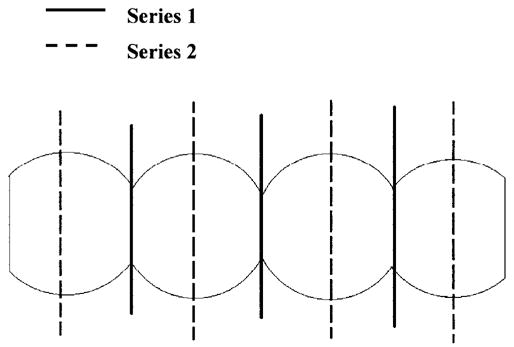
Series 1 and series 2 have the same between-slice intervals. Volume estimated by series 1 will be the smallest, whereas the volume estimated by series 2 will be the largest. Because both the smallest and the largest estimated volumes are within one group of the same interval but different starting points, it is possible for this group to have a high CV. Were the intervals slightly larger, the estimated volumes would not include the smallest and the largest estimated volume. Thus, the CV of a group with a larger interval may be smaller than the CV of a group with a smaller interval.

When evaluating the reproducibility of segmentation of imaging methods, previous studies reported between-analyzer and intra-analyzer CVs in identifying the area of interest in each slice (25–27). The CVs in these studies are caused by individual analyzer variability and will vary among laboratories and analyzers. The CVs calculated and discussed in the present study are caused by design considerations and do not vary among laboratories or analyzers.

Conclusions

Equation 5 is more accurate for estimating the regional and whole-body tissue volume than Equation 4 in the VW when intervals are set at 10, 20, 30, 40, 50, 60, 70, or 80 mm and slice thickness is set at 10 mm. In other words, the parallel trapezium model and the two-column model are more accurate in estimating tissue volumes than the truncated pyramid model and the truncated cone model. Although there is no need to question the previous studies that adopted Equation 4, Equation 5 is recommended for future studies. The accuracy of Equation 5 should be further validated by continuous scans of human subjects differing in weight, height, sex, and age.

Nonstandard abbreviations

CT

computerized axial tomography

MRI

magnetic resonance imaging

VW

visible woman

SAT

subcutaneous adipose tissue

VAT

visceral adipose tissue

SM

skeletal muscle

CV

coefficient of variation

Appendix 1

The mean volume from Equation 5 is always equivalent to the true volume and can be proven mathematically. The following calculations’ units are in millimeters.

For example, assume that the total length of one compartment is 100 mm; thus, the total number of slices is 100. The true volume is:

$$V_r=\sum _{i=1}^N(1\times A_i)=\sum _{i=1}^{100}(1\times A_i)=\sum _{i=1}^{100}{A}_i$$

When the slice interval is 10 mm, because the total number of starting points equals the sum of slice thickness and between-slice interval, there are 20 starting points.

With Equation 5 as:

$$V_i=(t+h)\sum _{i=1}^N{A}_i,$$

Then the 20 estimation volumes are:

$$\begin{array}{l}{V}_1=(10+10)(A_1+A_{21}+A_{41}+A_{61}+A_{81});\\ V_2=(10+10)(A_2+A_{22}+A_{42}+A_{62}+A_{82});\\ V_3=(10+10)(A_3+A_{23}+A_{43}+A_{63}+A_{83});\\ V_4=(10+10)(A_4+A_{24}+A_{44}+A_{64}+A_{84});\\ \cdots \\ \cdots \\ \cdots \\ V_{17}=(10+10)(A_{17}+A_{37}+A_{57}+A_{77}+A_{97});\\ V_{18}=(10+10)(A_{18}+A_{38}+A_{58}+A_{78}+A_{98});\\ V_{19}=(10+10)(A_{19}+A_{39}+A_{59}+A_{79}+A_{99});\\ V_{20}=(10+10)(A_{20}+A_{40}+A_{60}+A_{80}+A_{100});\\ \overline{V}=(10+10)(V_1+V_2+V_3+V_4+\dots +V_{17}+V_{18}+V_{19}+V_{20})/20\\ =(V_1+V_2+V_3+V_4+\dots +V_{17}+V_{18}+V_{19}+V_{20})\\ =(A_1+A_2)+A_3+A_4+\dots +A_{97}+A_{98}+A_{99}+A_{100})=\sum _{i=1}^{100}{A}_i\end{array}$$

Thus, V̄ = V_r.

With varying numbers of total slices and different between-slice intervals, the deduction is similar to the above procedures and V̄ is always equal to V_r.

Appendix 2

The combined volume of muscle and adipose tissue can be calculated by two methods.

A₁ and A₂ are the areas of muscle of adjacent slices. A₃ and A₄ are the areas of adipose tissue of adjacent slices.

For V₁, the volumes of muscle and adipose tissue are calculated by an equation and the volumes are summed to obtain combined volume.

For V₂, A₁ and A₃ are summed first to provide the total area of one slice, A₂ and A₄ are summed to provide the total area of another slice, and the combined volume is then calculated by an equation with the total areas. Equation 4:

$$\begin{array}{l}{V}_1=h(A_1+A_2+\sqrt{A_1{A}_2})/3+h(A_3+A_4+\sqrt{A_3{A}_4})/3\\ V_2=h[(A_1+A_3)+(A_2+A_4)+\sqrt{(A_1+A_3)(A_2+A_4)}]/3\\ V_1-V_2=h[\sqrt{(A_1+A_3)(A_2+A_4)}-\sqrt{A_1{A}_2}-\sqrt{A_3{A}_4}]/3\\ =\frac{[\sqrt{(A_1+A_3)(A_2+A_4)}+(\sqrt{A_1{A}_2}+\sqrt{A_3{A}_4})]}{\sqrt{(A_1+A_3)(A_2+A_4)}+(\sqrt{A_1{A}_2}+\sqrt{A_3{A}_4})}\\ \times [\sqrt{(A_1+A_3)(A_2+A_4)}-(\sqrt{A_1{A}_2}+\sqrt{A_3{A}_4})]\times \frac{h}{3}\\ =\frac{(A_1+A_3)(A_2+A_4)-{(\sqrt{A_1{A}_2}+\sqrt{A_3{A}_4})}^2}{\sqrt{(A_1+A_3)(A_2+A_4)}+(\sqrt{A_1{A}_2}+\sqrt{A_3{A}_4})}\times \frac{h}{3}\\ =\frac{A_1{A}_4+A_3{A}_2-2\sqrt{A_1{A}_2}\sqrt{A_3{A}_4}}{\sqrt{(A_1+A_3)(A_2+A_4)}+\sqrt{A_1{A}_2}+\sqrt{A_3{A}_4}}\times \frac{h}{3}\\ =\frac{{(\sqrt{A_1{A}_4}-\sqrt{A_3{A}_2})}^2}{\sqrt{(A_1+A_3)(A_2+A_4)}+\sqrt{A_1{A}_2}+\sqrt{A_3{A}_4}}\times \frac{h}{3}\\ \ge 0\end{array}$$

Thus, V₁ ≥ V₂

Equation 5:

$$\begin{array}{l}{V}_1=h(A_1+A_2)/2+h(A_3+A_4)/2\\ V_2=h[(A_1+A_3)+(A_2+A_4)]/2\end{array}$$

Thus, V₁ = V₂

References

- 1.Heymsfield SB, Ross R, Wang Z, Frager D. Imaging technique of body composition. Advantages of measurement and new uses. In: Carlson-Newberry SJ, Costello RB, editors. Imaging Technologies for Nutrition Research. Washington, DC: National Academy Press; 1997. pp. 127–50. [Google Scholar]
- 2.Ross R, Léger L, Morris D, de Guise J, Guardo R. Quantification of adipose tissue by MRI: relationship with anthropometric variables. J Appl Physiol. 1992;72:787–95. doi: 10.1152/jappl.1992.72.2.787. [DOI] [PubMed] [Google Scholar]
- 3.Ross R, Shaw KD, Rissanen J, Martel Y, de Guise J, Avruch L. Sex differences in lean and adipose tissue distribution by magnetic resonance imaging: anthropometric relationships. Am J Clin Nutr. 1994;59:1277–85. doi: 10.1093/ajcn/59.6.1277. [DOI] [PubMed] [Google Scholar]
- 4.Ross R. Magnetic resonance imaging provides new insights into the characterization of adipose and lean tissue distribution. Can J Physiol Pharmacol. 1996;74:778–85. [PubMed] [Google Scholar]
- 5.Anderson PJ, Chan JC, Chan YL, et al. Visceral fat and cardiovascular risk factors in Chinese NIDDM patients. Diabetes Care. 1997;20:1854–8. doi: 10.2337/diacare.20.12.1854. [DOI] [PubMed] [Google Scholar]
- 6.Thomas EL, Brynes AE, McCarthy J, et al. Preferential loss of visceral fat following aerobic exercise, measured by magnetic resonance imaging. Lipids. 2000;35:769–76. doi: 10.1007/s11745-000-0584-0. [DOI] [PubMed] [Google Scholar]
- 7.Kvist H, Sjöström L, Tylen U. Adipose tissue volume determinations in women by computed tomography: technical considerations. Int J Obes. 1986;10:53–67. [PubMed] [Google Scholar]
- 8.The U.S. National Library of Medicine. Visible Human Project. 1995. Visible Human CD-ROM. Version 1.1. [Google Scholar]
- 9.Tang H, Vasselli J, Wu EX, Gallagher D. In vivo determination of body composition of rats using high resolution magnetic resonance imaging. Ann N Y Acad Sci. 2000;904:32–41. doi: 10.1111/j.1749-6632.2000.tb06418.x. [DOI] [PubMed] [Google Scholar]
- 10.Tang H, Vasselli J, Wu EX, Boozer CN, Gallagher D. High resolution magnetic resonance imaging tracks changes in organ and tissue mass in rats. Am J Physiol Regul Integr Comp Physiol. 2002;282:R890–9. doi: 10.1152/ajpregu.0527.2001. [DOI] [PubMed] [Google Scholar]
- 11.Busetto L, Tregnaghi A, Bussolotto M, et al. Visceral fat loss evaluated by total body magnetic resonance imaging in obese women operated with laparascopic adjustable silicone gastric banding. Int J Obes Relat Metab Disord. 2000;24:60–69. doi: 10.1038/sj.ijo.0801086. [DOI] [PubMed] [Google Scholar]
- 12.Jones PR, Pearson J. Anthropometric determination of leg fat and muscle plus bone volumes in young male and female adults. J Physiol. 1969;204:63P–66P. [PubMed] [Google Scholar]
- 13.Engelson ES, Kotler DP, Tan Y, et al. Fat distribution in HIV-infected patients reporting truncal enlargement quantified by whole-body magnetic resonance imaging. Am J Clin Nutr. 1999;69:1162–9. doi: 10.1093/ajcn/69.6.1162. [DOI] [PubMed] [Google Scholar]
- 14.Janssen I, Ross R. Effects of sex on the change in visceral, subcutaneous adipose tissue and skeletal muscle in response to weight loss. Int J Obes Relat Metab Disord. 1999;23:1035–46. doi: 10.1038/sj.ijo.0801038. [DOI] [PubMed] [Google Scholar]
- 15.Rice B, Janssen I, Hudson R, Ross R. Effects of aerobic or resistance exercise and/or diet on glucose tolerance and plasma insulin levels in obese men. Diabetes Care. 1999;22:684–91. doi: 10.2337/diacare.22.5.684. [DOI] [PubMed] [Google Scholar]
- 16.Rissanen J, Hudson R, Ross R. Visceral adiposity, androgens, and plasma lipids in obese men. Metabolism. 1994;43:1318–23. doi: 10.1016/0026-0495(94)90229-1. [DOI] [PubMed] [Google Scholar]
- 17.Ross R, Rissanen J, Pedwell H, Clifford J, Shragge P. Influence of diet and exercise on skeletal muscle and visceral adipose tissue in men. J Appl Physiol. 1996;81:2445–55. doi: 10.1152/jappl.1996.81.6.2445. [DOI] [PubMed] [Google Scholar]
- 18.Kvist H, Chowdhury B, Grangård U, Tylén U, Sjöström L. Total and visceral adipose-tissue volumes derived from measurements with computed tomography in adult men and women: predictive equations. Am J Clin Nutr. 1988;48:1351–61. doi: 10.1093/ajcn/48.6.1351. [DOI] [PubMed] [Google Scholar]
- 19.Shih R, Wang Z, Heo M, Wang W, Heymsfield SB. Lower limb skeletal muscle mass: development of dual-energy X-ray absorptiometry prediction model. J Appl Physiol. 2000;89:1380–6. doi: 10.1152/jappl.2000.89.4.1380. [DOI] [PubMed] [Google Scholar]
- 20.Sjöström L, Kvist H, Cederblad Å, Tylén U. Determination of total adipose tissue and body fat in women by computed tomography, 40K, and tritium. Am J Physiol. 1986;250:E736–45. doi: 10.1152/ajpendo.1986.250.6.E736. [DOI] [PubMed] [Google Scholar]
- 21.Thomas EL, Saeed N, Hajnal JV, et al. Magnetic resonance imaging of total body fat. J Appl Physiol. 1998;85:1778–85. doi: 10.1152/jappl.1998.85.5.1778. [DOI] [PubMed] [Google Scholar]
- 22.Wang W, Wang Z, Faith MS, Kotler D, Shih R, Heymsfield SB. Regional skeletal muscle measurement: evaluation of new dual-energy X-ray absorptiometry model. J Appl Physiol. 1999;87:1163–71. doi: 10.1152/jappl.1999.87.3.1163. [DOI] [PubMed] [Google Scholar]
- 23.Wang ZM, Visser M, Ma R, et al. Skeletal muscle mass: evaluation of neutron activation and dual-energy X-ray absorptiometry methods. J Appl Physiol. 1996;80:824–31. doi: 10.1152/jappl.1996.80.3.824. [DOI] [PubMed] [Google Scholar]
- 24.Wang Z, Heo M, Lee RC, Kotler DP, Withers RT, Heymsfield SB. Muscularity in adult humans: proportion of adipose tissue-free body mass as skeletal muscle. Am J Human Biol. 2001;13:612–9. doi: 10.1002/ajhb.1099. [DOI] [PubMed] [Google Scholar]
- 25.Björntorp P. Portal” adipose tissue as a generator of risk factors for cardiovascular disease and diabetes. Arteriosclerosis. 1990;10:493–6. [PubMed] [Google Scholar]
- 26.Elbers JM, Haumann G, Asscheman H, Seidell JC, Gooren LJ. Reproducibility of fat area measurements in young, non-obese subjects by computerized analysis of magnetic resonance images. Int J Obes Relat Metab Disord. 1997;21:1121–9. doi: 10.1038/sj.ijo.0800525. [DOI] [PubMed] [Google Scholar]
- 27.Seidell JC, Bakker CJ, van der Kooy K. Imaging techniques for measuring adipose-tissue distribution–a comparison between computed tomography and 1.5-T magnetic resonance. Am J Clin Nutr. 1990;51:953–7. doi: 10.1093/ajcn/51.6.953. [DOI] [PubMed] [Google Scholar]