Functional Tissue Pulsatility Imaging of the Brain during Visual Stimulation

Abstract

Functional tissue pulsatility imaging (fTPI) is a new ultrasonic technique being developed to map brain function by measuring changes in tissue pulsatility due to changes in blood flow with neuronal activation. The technique is based in principle on plethysmography, an older, non-ultrasound technology for measuring expansion of a whole limb or body part due to perfusion. Perfused tissue expands by a fraction of a percent early in each cardiac cycle when arterial inflow exceeds venous outflow and relaxes later in the cardiac cycle when venous drainage dominates. Tissue pulsatility imaging (TPI) uses tissue Doppler signal processing methods to measure this pulsatile “plethysmographic” signal from hundreds or thousands of sample volumes in an ultrasound image plane. A feasibility study was conducted to determine if TPI could be used to detect regional brain activation during a visual contrast-reversing checkerboard block paradigm study. During a study, ultrasound data were collected transcranially from the occipital lobe as a subject viewed alternating blocks of a reversing checkerboard (stimulus condition) and a static, gray screen (control condition). Multivariate Analysis of Variance (MANOVA) was used to identify sample volumes with significantly different pulsatility waveforms during the control and stimulus blocks. In 7 out 14 studies, consistent regions of activation were detected from tissue around the major vessels perfusing the visual cortex.

INTRODUCTION

As early as the 1870s it was observed that mental activity influences regional brain physiology (Raichle 1998). Several researchers demonstrated that the surface pulsations and the temperature of the brain increase with mental activity (Raichle 1998). The technology necessary to pursue this research was limited, and it was not until the 1950s that the first instrument for quantifying whole brain blood flow and metabolism in humans was developed (Landau et al. 1956). Though the mechanisms coupling neuronal activation and vascular response are not fully understood, it is generally accepted that neural activation triggers vasodilation of the supplying vessels thereby increasing blood flow to activated areas in the brain (Girouard and Iadecola 2006).

Various modalities have been developed for functional brain imaging. Techniques such as electroencephalography (EEG) and magenetoencephalography (MEG) measure the electromagnetic fields produced during neuronal activation to map brain function (Darvas et al. 2004; George et al. 1995). Other techniques such as functional near-infrared spectroscopy (fNIRS) (Plichta et al. 2006), functional magnetic resonance imaging (fMRI) (Matthews 2002), positron emission tomography (PET) (Turner and Jones 2003), single photon emission computed tomography (SPECT) (Wyper 1993), and functional transcranial Doppler sonography (fTCD) (Stroobant and Vingerhoets 2000) measure changes in blood flow or blood gas concentration as surrogates for changes in neuronal activation.

The introduction of transcranial Doppler sonography (TCD) provided a non-invasive means to monitor blood flow through the major cerebral vessels in real-time (Aaslid et al. 1982). Functional TCD is the application of TCD for monitoring task-specific changes in cerebral blood flow. Early studies in fTCD focused on arterial velocity changes evoked through a simple light stimulation of the eye (Aaslid 1987; Conrad and Klingelhöfer 1989). Significant velocity changes were observed, particularly in the posterior cerebral artery (PCA), the principal vessel supplying the primary visual cortex. The range of studies has since expanded to include colored light, field-of-vision, half-field stimulation, intermittent stimulation, and stimulation with complex images (Klingelhöfer et al. 1999, Stroobant and Vingerhoets 2000). Changes in blood flow through the middle cerebral artery (MCA) associated with a specific stimulation have also been demonstrated. These studies focused more on auditory stimulation, cognitive tasks, language, memory tests, and motor tasks (Klingelhöfer et al. 1999, Stroobant and Vingerhoets 2000). These studies were validated through direct comparison against the Wada test, which uses an anesthetic for lateral suspension of brain activity (Strauss et al. 1985), and against fMRI establishing fTCD as a viable complementary tool for functional brain imaging (Binder et al. 1996; Deppe et al. 2000; Desmond et al. 1995; Knecht et al. 1998). Functional TCD has since been applied to the study of migraines (De Benedittis et al. 1999; Backer et al. 2001), stroke recovery (Bragoni et al. 2000; Matteis et al. 2003), Alzheimer’s disease (Asil and Uzuner 2005), Parkinson’s disease (Troisi et al. 2002), Huntington’s disease (Deckel and Cohen 2000) and schizophrenia (Sabri et al. 2003; Feldmann et al. 2006).

Compared to other brain imaging systems such as PET, SPECT, and MRI, TCD is a rapid, portable, inexpensive, continuous monitoring technique that can be applied to subjects and in settings unsuitable for study by other neuroimaging techniques. Functional TCD is limited, however, in its ability to localize regions of activity; TCD can only be used to measure flow through larger segments of the cerebral vasculature that supply blood to large regions of the brain spanning multiple functional areas because the signal backscattered by blood is significantly less than that backscattered by tissue. In addition, the skull significantly attenuates ultrasound (US); Fry and Barger (1978) reported the attenuation of the skull to be 13 dB/cm/MHz. Therefore, to measure blood flow, TCD is generally limited to application through the three “acoustic windows”, the temporal bone window, the orbital window, and the foramen magnum window. This again, however, limits the regional access available with fTCD. Furthermore, 5–8% of the population does not have an adequate acoustic window (Deppe 2005; White and Venkatesh 2006).

At the University of Washington we are developing a functional ultrasonic imaging method, referred to as functional tissue pulsatility imaging (fTPI), that measures the natural pulsatile motion of tissue due to blood flow as a surrogate for blood flow itself. By measuring tissue motion and/or tissue strain (the derivative of motion with depth) rather than blood velocity, we are able to overcome the limitation of low backscatter from blood that limits US access to the skull’s acoustic windows. We have validated the technique by measuring the hemodynamic response associated with visual stimulation of the occipital cortex using a contrast-reversing checkerboard paradigm.

Tissue pulsatility imaging (TPI) is a variation of tissue Doppler imaging (Eriksson et al. 2002; McDicken et al. 1992) developed in our laboratory to characterize blood flow and perfusion by measuring the natural tissue expansion and relaxation over the cardiac and respiratory cycles (Beach et al. 1992, 1993, 1994; Kucewicz et al. 2004). During systole, blood enters tissue through the arterial vasculature faster than it leaves through the venous vasculature causing blood to accumulate and the tissue to expand by a fraction of a percent. During diastole, venous drainage dominates allowing the tissue to return to its presystolic volume. The rate of venous drainage is modulated by the respiratory cycle if the tissue is not elevated above the chest. This results in a periodic expansion of nearly one percent synchronized with respiration in addition to the cardiac pulsatile expansion (Strandness and Sumner 1975).

TPI is based in principle on a much older, established technique called plethysmography (Strandness 1965, Strandness and Sumner 1975, Sumner 1993). Plethysmography has been a popular noninvasive diagnostic method for the assessment of arterial and venous disease since the 1960’s. The technique works by measuring whole limb expansion due to vascular perfusion in association with the cardiac cycle (arterial) or the respiratory cycle (venous). With TPI, US is used to measure tissue displacement or strain to provide the “plethysmographic” signal from hundreds or thousands of small volumes of tissue within an US image plane rather than the gross plethysmographic signal from the entire limb or body part as is done with traditional plethysmography.

MATERIALS AND METHODS

Subjects

Two subjects participated in the study, a 34 year-old, right-handed male and a 39 year-old, left-handed female. Both subjects had normal, uncorrected vision. A total of seven sessions were conducted on each subject over a four week period. For each session, the two subjects were studied on the same day, approximately 30 minutes apart. No effort was made to control day of the week, time of day, or caffeine intake. Written informed consent was obtained from both subjects. The research protocol was approved by the Human Subjects Committee of the University of Washington. Full 3D anatomical and angiographic MRI data were collected on the male subject as part of another approved study and were used to identify the location of the occipital lobe and other structures in the brain.

Protocol

During a study, the subject lay prone on a massage table (Stronglite, Inc., Cottage Grove, OR) with his/her head securely and comfortably positioned within the table’s face donut. ECG leads were attached to the subject’s arms, and US gel was applied to the back of the subject’s head. A Terason 4V2 phased-array transducer (Teratech Corp., Burlington, MA) held by an articulated clamp (Manfrotto, Bassano del Grappa, Italy) securely mounted to a laboratory bench was positioned on the back of the head over the visual cortex approximately 2 cm superior to the occipital protuberance and 0 to 2 cm lateral from the midline (Fig. 1). Before locking the clamp in place, the transducer was oriented by an experienced sonographer to image a nearly transverse plane passing through the pineal body, which is hyperechoic in most individuals due to calcification. The visual stimuli were displayed on a computer monitor (Dell Latitude D610, Round Rock, TX) approximately 75 cm directly below the subject’s face. Prior to the start of the study, the lights were dimmed and a visual shield was placed around the front of the table to minimize visual distractions.

Fig. 1.

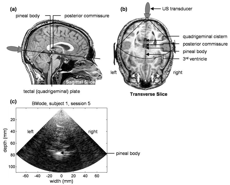
(a,b) MRI images showing the position and orientation of the US transducer. (c) BMode image from the male subject. The black sector shown in (b) represents the approximate location and extent of the BMode image.

A contrast-reversing checkerboard block paradigm was used to stimulate the visual cortex. This is a robust test that reliably produces a response independent of cognitive or learning processes (DeYoe et al. 1994). Each study consisted of 31 alternating control and checkerboard blocks beginning and ending with a control block. During a checkerboard block, an 8 square x 8 square black-and-white checkerboard was displayed for 30 s with the squares alternating from black to white or white to black every 500 ms. Each square measured 2 cm x 2 cm creating a 16 cm x 16 cm checkerboard. During a control block, a static gray screen was displayed for 30 s.

Data Acquisition

The data acquisition system (Fig. 2) consisted of a Terason 2000 US scanner (Teratech Corp., Burlington, MA), a personal computer for displaying the visual stimuli, a personal computer for digitizing the subject’s ECG signal, an ECG monitor (VSM2, Physio-Control, Redmond, WA), and an arbitrary waveform generator (33120A, Agilent Technologies, Palo Alto, CA) controlled by the visual stimulation computer for triggering the US scanner and ECG digitizer. The output of the ECG monitor was a TTL signal coincident with the subject’s ECG R-wave.

Fig. 2.

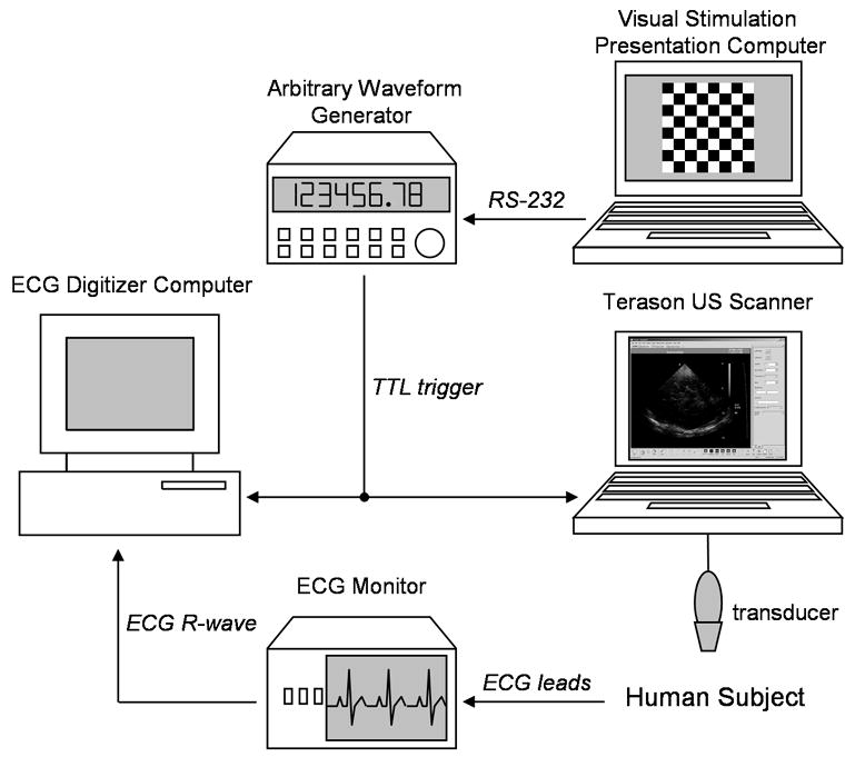
Data collection hardware schematic.

The Terason 2000, a laptop-based, general-purpose US scanner, with the 4V2 phased array scanhead (90° sector angle, 64 element, 2.5 MHz center frequency, 10 MHz RF sampling frequency, 128 scanlines per frame, approximately 55% fractional bandwidth BMode pulse) was used for US acquisition. With software provided by the manufacturer, a series of post-beamformed US radio frequency (RF) frames were collected during BMode imaging for offline analysis in MATLAB (The Mathworks, Inc., Natick, MA). A total of 240 frames of RF US were recorded at 30 frames per second from 10 s to 18 s within each block. With the Terason, we are able to record up to 300 frames of RF US. Only 240 frames were recorded to allow sufficient time to write the data to the Terason’s hard drive. Data collection was started 10 s into each block to allow sufficient time for the blood flow to change in response to the neuronal stimulation (Aaslid 1987). To automate the data collection on the Terason, AutoHotkey (http://www.autohotkey.com) was used to arm the Terason and save data at the appropriate times without user intervention once the session was started.

A MATLAB script running on the Dell Latitude D610 laptop computer was used to display the visual stimuli and synchronize data acquisition by the other two computers (Fig. 3). Ten seconds into each stimulus block, the MATLAB script instructed the arbitrary waveform generator to output a 100 ms TTL pulse that triggered the Terason (using the Terason’s ECG triggering feature) and the ECG digitizer computer. The subject’s ECG R-wave signal was digitized using a Measurement Computing (Middleboro, MA) PCI-DAS 1000 12-bit digitizer sampling at 1 kHz. Eight seconds after each trigger, the two computers recorded their data to hard drives and rearmed before the next trigger.

Fig. 3.

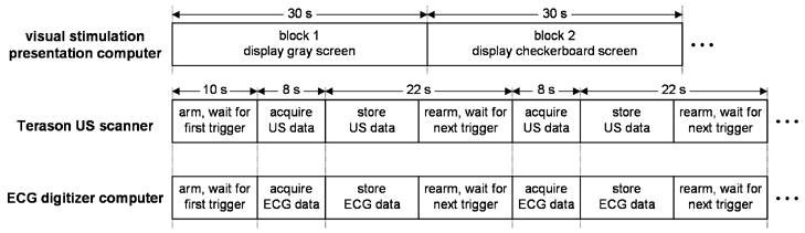
Data collection timing diagram. Ten seconds into each block the visual stimulation presentation computer instructed the arbitrary waveform generator to output a 100 ms TTL pulse that triggered acquisition of the US and ECG data.

Displacement Estimation

The data analysis steps are shown in Fig. 4. The analytic versions of the post-beamformed RF US signals were first calculated using the Hilbert transform. From the analytic signals, tissue displacement was measured using the 2D autocorrelation estimator (Loupas et al. 1995). The standard 1D autocorrelator estimates the mean change in phase of the quadrature demodulated or analytic signal in slow-time, i.e. pulse-to-pulse, and scales the result by the wavelength of US at a reference frequency, typically the transmitted US center frequency, to derive velocity or displacement (Kasai et al. 1985). The limitation of this method is that the result is biased by stochastic variation of the US center frequency (Bonnefous and Pesque 1986) and frequency-dependent attenuation (Ferrara et al. 1992). The 2D autocorrelator additionally estimates the mean change in phase of the signal in fast-time, i.e. depth-to-depth, to calculate the local US center frequency and uses the wavelength at that frequency to derive velocity or displacement. With the 2D autocorrelator, displacement is estimated as:

Fig. 4.

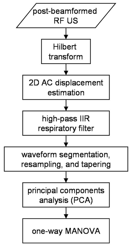
Data analysis flow diagram.

$${\widehat{d}}_{2D}=\frac{c}{2}\frac{\frac{1}{2\pi }arg\{{\widehat{R}}_a(0,T)\}}{\frac{1}{2\pi t_s}arg\{{\widehat{R}}_a(t_s,0)\}}$$ (1)

where c is the speed of US in soft tissue, T is the pulse-to-pulse sampling period, ^ts is the depth-to-depth sampling period, R̂_a (r, τ) is the estimate of the complex 2D autocorrelation function at depth lag r and temporal lag τ, and “arg” is the argument, i.e. phase angle, of R̂_a (r, τ) . If the complex autocorrelation is expanded, eqn (1) for a particular sample volume with a depth lag of 1 sample and with a temporal lag of 1 sample can be written as:

$${\widehat{d}}_{2D}=\frac{c}{2}\frac{\frac{1}{2\pi }arg\left({\displaystyle \sum _{i=1}^I}{\displaystyle \sum _{j=1}^J}{\displaystyle \sum _{k=2}^K}Z(i,j,k)Z^{\ast }(i,j,k-1)\right)}{\frac{1}{2\pi t_s}arg\left({\displaystyle \sum _{i=2}^I}{\displaystyle \sum _{j=1}^J}{\displaystyle \sum _{k=1}^K}Z(i,j,k)Z^{\ast }(i-1,j,k)\right)}$$ (2)

where Z is the analytic signal indexed by depth i, scan line j, and frame k and where I, J, and K indicate the number of depths, scan lines, and frames, respectively, over which the measurement is made. For this work, we used I=10 (0.77 mm), J=2 (0.025 rad), and K=2 (2 frames). Displacement for the first frame was set to 0, and displacement for subsequent frames was calculated from the cumulative displacement from previous frames (Kucewicz et al. 2004).

Data Conditioning

The displacement waveforms for all of the sample volumes were first forward and reverse filtered to remove respiratory motion using a 3^rd order, high-pass Butterworth IIR filter with a cutoff at three-quarters of the mean cardiac frequency during the 8 s data block. Mean cardiac frequency was calculated from the subject’s ECG R-wave intervals recorded concurrently with the US data.

Using the ECG R-waves, the displacement waveforms were segmented into their individual cardiac cycles and resampled (Fig. 5). Each cardiac cycle was segmented using the last sample preceding its R-wave and the first sample following the next cardiac cycle’s R-wave. Cardiac cycles that began 0.5 s into the data block or ended 0.5 s from the end of the data block were not used because of start-up and ending transient effects introduced by the respiratory filter typically leaving five or six complete cardiac cycles during each block. The segments were then resampled by linear interpolation at 30 Hz such that the first time point in each resampled displacement waveform coincided in time with the cycle’s R-wave. Each resampled segment was shifted such that the displacement at the beginning of the cardiac cycle was 0.

Fig. 5.

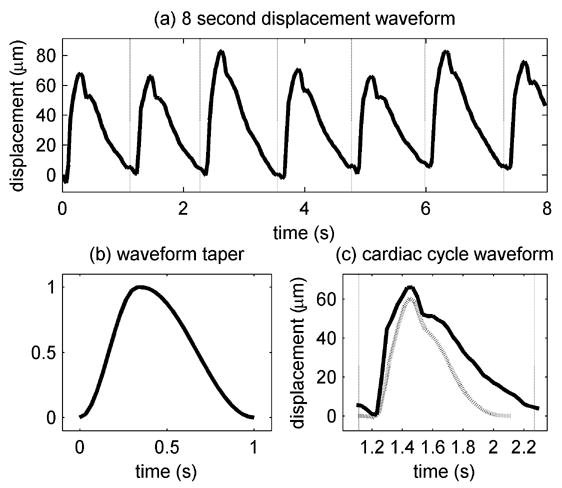
Displacement waveforms and taper. (a) 8 s displacement waveform during a control block for a sample volume near the brain stem after filtering for respiratory motion. The vertical dotted lines indicate the beginnings of the cardiac cycles based on the ECG R-waves. (b) Modified 31 sample Hann window. (c) One cardiac cycle (solid line) from (a) and the waveform after tapering (dotted line).

Each displacement waveform segment for each cardiac cycle was tapered to 1 s to compensate for the variable durations of the cardiac cycles to allow all of the cardiac cycles to be compared as described in subsequent sections. A modified 31 sample Hann window was used to taper the displacement waveforms (Fig. 5). The first 11 samples within each segment were tapered using the first 11 points of a 21 point Hann window, and the remaining 20 samples were tapered using the last 20 points of a 40 point Hann window. This window was created such that the peak of the windowing function approximately coincided with the systolic peak in the displacement waveform segments. The displacement waveform segments for cardiac cycles less than 1 s were zero-padded before tapering. Both subjects have resting heart rates less than 60 beats-per-minute so relatively few cycles needed to be zero-padded. The displacement waveforms were then spatially filtered using a Gaussian filter with a full-width-at-half-maximum (FWHM) of 4 mm.

Feature Extraction and Statistical Analysis

Multivariate Analysis of Variance (MANOVA) applied independently to each sample volume was used to test the null hypothesis that the means of the groups of displacement waveforms collected during the control blocks and stimulus blocks were the same (Green 1978). Before applying MANOVA, Principal Components Analysis (PCA) was used to reduce the dimensionality of the data.

PCA is standard statistical technique commonly used for feature extraction and data reduction (Green 1978). PCA is a linear transform that projects multivariate data onto new coordinate axes, i.e. new variables, that are ordered by the amount of variance in the original data that they explain. If the original variables are highly correlated, the number of variables can be reduced by eliminating the new variables that do not account for a significant fraction of the variance.

The displacement waveforms for each sample volume were first organized into an M row by N column matrix, X, where M corresponds to the number of samples in each cardiac cycle and N corresponds to the number of cardiac cycles from all blocks for the entire study. A typical study consisted of 150 to 170 cardiac cycles. For this analysis, the displacement waveform for each cardiac cycle was treated in effect as a variable with 31 dimensions (M=31). Each row’s mean was subtracted to yield the mean-corrected matrix, B, from which the covariance matrix, C, was calculated:

$$\mathbf{C}=\frac{1}{N-1}\mathbf{B}·{\mathbf{B}}^{\prime }$$ (3)

The eigenvector matrix, V, and the eigenvalue matrix, D, of C were then calculated:

$$\mathbf{C}·\mathbf{V}=\mathbf{V}·\mathbf{D}$$ (4)

D is the MxM diagonal matrix of eigenvalues sorted in descending order where each eigenvalue indicates the variance of the original data when projected onto the corresponding eigenvector arranged in columns in the MxM matrix V. The cumulative fractional energy in the first L eigenvectors is defined as:

$$g[L]=\frac{{\displaystyle \sum _{l=1}^L}D[l,l]}{{\displaystyle \sum _{m=1}^M}D[m,m]}$$ (5)

The cumulative fractional energy can be used for dimensionality reduction by retaining the first L eigenvectors needed to exceed a variance threshold for g. For this work a threshold of 95% was used. A new MxL matrix, W, was constructed containing the first L eigenvectors. Lastly, the original data were projected onto W:

$$\mathbf{Y}={\mathbf{W}}^{\prime }·\mathbf{B}$$ (6)

where Y is the LxN matrix of principal components, i.e. Y[l,n] corresponds to the projection of the n^th displacement waveform onto the l^th eigenvector.

The principal components were then divided into two groups, the control group and the checkerboard group, and one-way MANOVA was used to test the null hypothesis that the groups have the same means. Reducing the number of variables by PCA before MANOVA has two benefits. Uncorrelated noise is expected to have a larger spread across the eigenvalue spectrum so eliminating lower variance eigenvectors improves the signal-to-noise ratio (SNR) of the data (Bjærum et al. 2002). Additionally, reducing the number of variables reduces the degrees of freedom thereby enhancing the statistical power of MANOVA (Green 1978).

RESULTS

Displacement waveforms for two control blocks and two checkerboard blocks for one sample volume are shown in Fig. 6. Within blocks and across blocks, the overall amplitude varies considerably due primarily to the influence of respiration on cardiac filling and resulting ejection fraction. Fig. 6b shows the mean displacement waveforms for the same sample volume for all of the control blocks and all of the checkerboard blocks. The shapes are remarkably similar, but the amplitude of the mean checkerboard waveform is larger than the amplitude of the mean control waveform as would be expected if the blood flow, and thereby the tissue pulsatility, increases during visual stimulation.

Fig. 6.

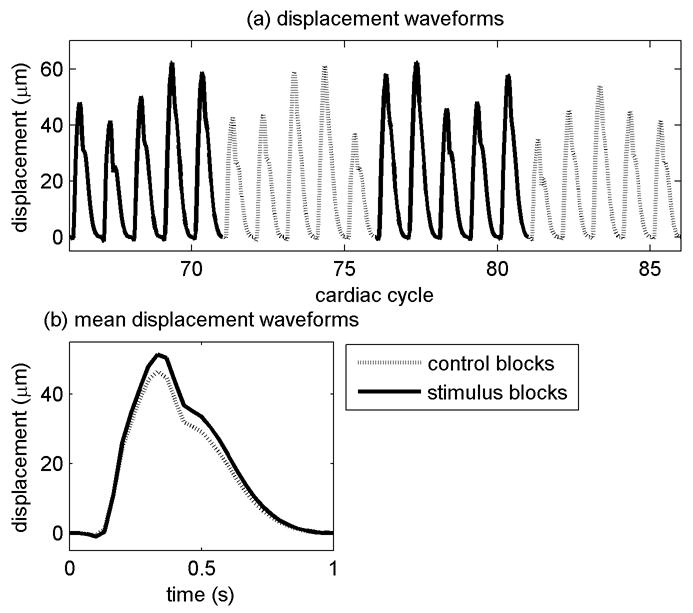
Displacement waveforms from one sample volume. (a) Displacement waveforms for four successive blocks. The waveforms have been resampled, tapered to 1 s and placed end-to-end. The entire data set consisted of 31 blocks and 157 cardiac cycles. (b) Mean waveforms from all of the cardiac cycles for the control blocks and the checkerboard blocks for the sample volume. For this sample volume, the p-value testing the hypothesis that the control blocks and checkerboard blocks have the same means was 1.0e-10.

Large regions of statistically significant activation during visual stimulation were detected in 4 of 7 studies for the male subject and in 3 of 7 studies for the female subject. For both subjects, the active regions consistently spanned the region around the pineal body (posterior P2 segment of the PCA) and the tissue extending posteriorly along the mid-line (P3 and P4 segments of the PCA). Fig. 7 shows the consistency in the results from the 4 successful studies for the male subject. The p-values calculated by MANOVA are shown super-imposed on BMode images for p-values less than 0.01. Fig. 8 shows the p-values for one of the sessions superimposed on an MRI image slice corresponding approximately to the US image plane.

Fig. 7.

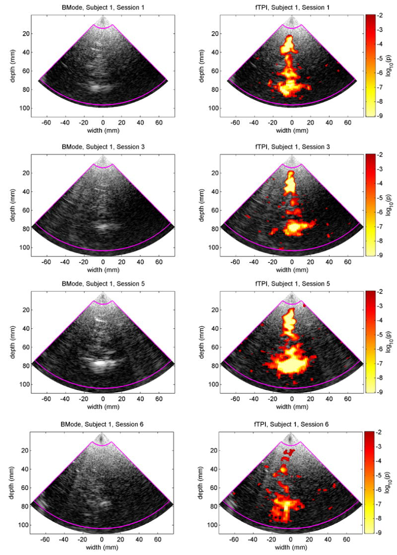
fTPI results for the 4 successful sessions for the male subject. The left column shows BMode images from one frame collected during each session. The brightest echo in each image at a depth of 80 mm is from the region around the pineal body. The right column shows the p-values for the fTPI data superimposed on the respective BMode images. P-values less that 0.01 are not considered significant and are not shown. The magenta boundary indicates the region-of-interest for the fTPI analysis.

Fig. 8.

MRI slice corresponding approximately to the US image plane with superimposed p-values from the male subject, session 5. The fTPI p-values have been drawn as a contour plot with curves every order of magnitude from 10⁻⁹ to 10⁻³.

DISCUSSION

In this study, we demonstrate a statistically significant increase in tissue pulsatility within the posterior region of the brain in response to a visual stimulus. The active regions appear to correlate with the paths of vessels that supply the visual cortex. A positive response was obtained in 4 out of 7 studies for the male subject and in 3 out of 7 studies for the female subject. The lack of response in the remaining studies could potentially be attributed to attentiveness; Schnittger et al. (1996) demonstrated a greater vascular response to a visual stimulus during periods of increased attentiveness. The study required the subject lay still in a prone position with his/her head within a massage table face donut. Both subjects expressed difficulty staying awake, lack of attentiveness, and fogging or tearing of the eyes at times. Passive viewing may not generate a sufficiently large response to be consistently detected by our system. To compensate for this, we could introduce a task that requires attentive interaction such as a reading test or symbol matching test. Though both these tasks would activate regions in addition to the visual cortex, if the response is more repeatable we would feel confident that attentiveness is an issue.

The ultrasound system used for the study may also have contributed to the variability in the response. This was a commercially available system with a phased array transducer that was not optimized for transcranial imaging. Therefore, the frequency and power settings are not optimized for our application. Furthermore, the transducer was a standard hand-held transducer retained by an articulated clamp. Although relatively stable, the long moment arm introduced some mechanical instability. A TCD system with a fitted transducer would be more appropriate and would allow the transducer to be held in place with a helmet-style fixture so the subject could sit in a more comfortable position during a study.

Because fTPI is based upon US, it maintains the qualities of being a rapid, portable, inexpensive tool that can be used for continuous monitoring and for repeat studies. The advantage of fTPI over fTCD is the use of tissue rather than blood as the signal source. US backscatter from tissue is significantly stronger than that from blood allowing acquisition of ultrasound signals of the cortical region of interest directly through the overlying skull. An additional advantage is the ability to study small functional cortical regions rather than larger arteries that supply multiple functional regions. For this study, we scanned through the skull over the occipital protuberance to guarantee we would be imaging through the visual cortex in the occipital lobe. The use of a tissue rather than blood backscatter signal may also result in an overall reduction in transmitted ultrasound power once the technique is optimized. The highest power outputs allowed by the FDA for diagnostic imaging are for TCD.

Additional work is being done to determine if tissue pulsatility is more appropriately measured using tissue strain rather than tissue displacement. Assessing regional brain activity using displacement is confounded by the cumulative motion of the brain, i.e. an increase in blood flow to a stimulated region of the brain might displace remote tissues making it appear as if they are activated even though they are not. Strain imaging could theoretically compensate for this remote, common-mode movement. Limited, preliminary analysis using strain waveforms measured using a least-squares strain estimator (Jackson and Thomas 2003) reveals similar regions of activation suggesting cumulative tissue displacement is not a significant problem.

CONCLUSIONS

In our study we have shown that fTPI is a potential technique for functional brain imaging. The light weight and small size natural to US scanners can permit functional brain imaging studies in ambulatory patients, a freedom prohibited by fMRI and nuclear imaging methods. Although functional EEG methods have comparable cost and portability, EEG lacks the spatial resolution of ultrasound. The electrical brain activity signals of EEG methods including evoked response potentials are complementary to the blood perfusion signals provided by the fTPI.

Currently we have collected data on two subjects over multiple sessions to establish the feasibility of the method. In the successful studies, we consistently observed regions of significantly increased tissue pulsatility extending posteriorly from the region of the pineal body to the occipital lobe through which pass the segments of the PCA that perfuse the primary visual cortex. Future work will determine if it is possible to detect differences in pulsatility in the cortex itself by refining the method and/or optimizing the US system for transcranial applications. Additional data will also be collected from more subjects to validate the method across a larger population of individuals.

References

- Aaslid R, Markwalder TM, Nornes H. Noninvasive transcranial Doppler ultrasound recording of flow velocity in basal cerebral arteries. J Neurosurg. 1982;57(6):769–74. doi: 10.3171/jns.1982.57.6.0769. [DOI] [PubMed] [Google Scholar]
- Aaslid R. Visually evoked dynamic blood flow response of the human cerebral circulation. Stroke. 1987;18(4):771–775. doi: 10.1161/01.str.18.4.771. [DOI] [PubMed] [Google Scholar]
- Asil T, Uzuner N. Differentiation of vascular dementia and Alzheimer disease: a functional transcranial Doppler ultrasonographic study. J Ultrasound Med. 2005;24(8):1065–1070. doi: 10.7863/jum.2005.24.8.1065. [DOI] [PubMed] [Google Scholar]
- Backer M, Sander D, Hammes MG, Funke D, Deppe M, Conrad B, Tolle TR. Altered cerebrovascular response pattern in interictal migraine during visual stimulation. Cephalalgia. 2001;21(5):611–616. doi: 10.1046/j.1468-2982.2001.00219.x. [DOI] [PubMed] [Google Scholar]
- Beach KW, Philips DJ, Kansky J. Ultrasonic plethysmograph. 5,088,498. US Patent #. 1992
- Beach KW, Philips DJ, Kansky J. Ultrasonic plethysmograph. 5,183,046. US Patent #. 1993
- Beach KW, Philips DJ, Kansky J. Ultrasonic plethysmograph. 5,289,820. US Patent #. 1994
- De Benedittis G, Ferrari Da Passano C, Granata G, Lorenzetti A. CBF changes during headache-free periods and spontaneous/induced attacks in migraine with and without aura: a TCD and SPECT comparison study. J Neurosurg Sci. 1999;43(2):141–6. [PubMed] [Google Scholar]
- Binder JR, Swanson SJ, Hammeke TA, et al. Determination of language dominance using functional MRI: a comparison with the Wada test. Neurology. 1996;46(4):978–984. doi: 10.1212/wnl.46.4.978. [DOI] [PubMed] [Google Scholar]
- Bjærum S, Torp H, Kristoffersen K. Clutter filters adapted to tissue motion in ultrasound color flow imaging. IEEE Trans Ultrason Ferroelectr Freq Control. 2002;49(6):693–704. doi: 10.1109/tuffc.2002.1009328. [DOI] [PubMed] [Google Scholar]
- Bonnefous O, Pesque P. Time domain formulation of pulse-Doppler ultrasound and blood velocity estimation by cross correlation. Ultrason Imaging. 1986;8(2):73–85. doi: 10.1177/016173468600800201. [DOI] [PubMed] [Google Scholar]
- Bragoni M, Caltagirone C, Troisi E, et al. Correlation of cerebral hemodynamic changes during mental activity and recovery after stroke. Neurology. 2000;55(1):35–40. doi: 10.1212/wnl.55.1.35. [DOI] [PubMed] [Google Scholar]
- Conrad B, Klingelhöfer J. Dynamics of regional cerebral blood flow for various visual stimuli. Exp Brain Res. 1989;77(2):437–441. doi: 10.1007/BF00275003. [DOI] [PubMed] [Google Scholar]
- Darvas F, Pantazis D, Kucukaltun-Yildirim E, Leahy RM. Mapping human brain function with MEG and EEG: methods and validation. Neuroimage. 2004;23 (Suppl 1):S289–299. doi: 10.1016/j.neuroimage.2004.07.014. [DOI] [PubMed] [Google Scholar]
- Deckel AW, Cohen D. Increased CBF velocity during word fluency in Huntington’s disease patients. Prog Neuropsychopharmacol Biol Psychiatry. 2000;24(2):193–206. doi: 10.1016/s0278-5846(99)00099-8. [DOI] [PubMed] [Google Scholar]
- Deppe M, Knecht S, Papke K, et al. Assessment of hemispheric language lateralization: a comparison between fMRI and fTCD. J Cereb Blood Flow Metab. 2000;20(2):263–288. doi: 10.1097/00004647-200002000-00006. [DOI] [PubMed] [Google Scholar]
- Desmond JE, Sum JM, Wagner AD, et al. Functional MRI measurement of language lateralization in Wada-tested patients. Brain. 1995;118( Pt 6):1411–1419. doi: 10.1093/brain/118.6.1411. [DOI] [PubMed] [Google Scholar]
- DeYoe EA, Bandettini P, Neitz J, Miller D, Winans P. Functional magnetic resonance imaging (FMRI) of the human brain. J Neurosci Methods. 1994;54(2):171–187. doi: 10.1016/0165-0270(94)90191-0. [DOI] [PubMed] [Google Scholar]
- Eriksson A, Greiff E, Loupas T, Persson M, Pesque P. Arterial pulse wave velocity with tissue Doppler Imaging. Ultrasound Med Biol. 2002;28(5):571–580. doi: 10.1016/s0301-5629(02)00495-7. [DOI] [PubMed] [Google Scholar]
- Feldmann D, Schuepbach D, von Rickenbach B, Theodoridou A, Hell D. Association between two distinct executive tasks in schizophrenia: a functional transcranial Doppler sonography study. BMC Psychiatry. 2006;6:25. doi: 10.1186/1471-244X-6-25. [DOI] [PMC free article] [PubMed] [Google Scholar]
- Ferrara KW, Algazi VR, Liu J. The effect of frequency dependent scattering and attenuation on the estimation of blood velocity using ultrasound. IEEE Trans Ultrason Ferroelectr Freq Control. 1992;39(6):754–767. doi: 10.1109/58.165561. [DOI] [PubMed] [Google Scholar]
- Fry FJ, Barger JE. Acoustical properties of the human skull. J Acoust Soc Am. 1978;63(5):1576–1590. doi: 10.1121/1.381852. [DOI] [PubMed] [Google Scholar]
- George JS, Aine CJ, Mosher JC, et al. Mapping function in the human brain with magnetoencephalography, anatomical magnetic imaging, and functional magnetic resonance imaging. J Clin Neurophysiol. 1995;12(5):406–431. doi: 10.1097/00004691-199509010-00002. [DOI] [PubMed] [Google Scholar]
- Girouard H, Iadecola C. Neurovascular coupling in the normal brain and in hypertension, stroke, and Alzheimer disease. J Appl Physiol. 2006;100(1):328–335. doi: 10.1152/japplphysiol.00966.2005. [DOI] [PubMed] [Google Scholar]
- Green PE. Analyzing Multivariate Data. Hinsdale, IL: The Dryden Press; 1978. [Google Scholar]
- Jackson JI, Thomas LJ. Application of ultrasound-based velocity estimate statistics to strain-rate estimation. IEEE Trans Ultrason Ferroelectr Freq Control. 2003;50(11):1464–1473. doi: 10.1109/tuffc.2003.1251130. [DOI] [PubMed] [Google Scholar]
- Kasai C, Namekawa A, Koyano A, Omato R. Real-time two-dimensional blood flow imaging using an autocorrelation technique. IEEE Trans Sonics Ultrason. 1985;32(3):458–464. [Google Scholar]
- Klingelhöfer J, Sander D, Wittich I. Functional Ultrasonic Imaging. In: Babikian VL, Wechsler LR, editors. Transcranial Doppler Ultrasonography. Woburn, MA: Butterworth-Heinemann; 1999. pp. 49–66. [Google Scholar]
- Knecht S, Deppe M, Ringelstein EB, et al. Reproducibility of functional transcranial Doppler sonography in determining hemispheric language lateralization. Stroke. 1998;29(6):1155–1159. doi: 10.1161/01.str.29.6.1155. [DOI] [PubMed] [Google Scholar]
- Kucewicz JC, Huang L, Beach KW. Plethysmographic arterial waveform strain discrimination by Fisher’s method. Ultrasound Med Biol. 2004;30(6):773–782. doi: 10.1016/j.ultrasmedbio.2004.04.002. [DOI] [PubMed] [Google Scholar]
- Landau WM, Freygang WH, Jr, Roland LP, Sokoloff L, Kety SS. The local circulation of the living brain; values in the unanesthetized and anesthetized cat. Trans Am Neurol Assoc. 1955–1956;(80th meeting):125–129. [PubMed] [Google Scholar]
- Loupas T, Powers JT, Gill RW. An axial velocity estimator for ultrasound blood flow imaging, based on a full evaluation of the Doppler equation by means of a two-dimensional autocorrelation approach. IEEE Trans Ultrason Ferroelectr Freq Control. 1995;42(4):672–688. [Google Scholar]
- Matteis M, Vernieri F, Troisi E, et al. Early cerebral hemodynamic changes during passive movements and motor recovery after stroke. J Neurol. 2003;250(7):810–817. doi: 10.1007/s00415-003-1082-4. [DOI] [PubMed] [Google Scholar]
- Matthews PM. An introduction to functional magnetic resonance imaging of the brain. In: Jezzard P, Matthews PM, Smith SM, editors. Functional MRI: an Introduction to Methods. Oxford, UK: Oxford University Press; 2002. pp. 1–34. [Google Scholar]
- McDicken WN, Sutherland GR, Moran CM, Gordon LN. Colour Doppler velocity imaging of the myocardium. Ultrasound Med Biol. 1992;18(6–7):651–654. doi: 10.1016/0301-5629(92)90080-t. [DOI] [PubMed] [Google Scholar]
- Plichta MM, Herrmann MJ, Baehne DG, et al. Event-related functional near-infrared spectroscopy (fNIRS): are the measurements reliable? Neuroimage. 2006;31(1):116–124. doi: 10.1016/j.neuroimage.2005.12.008. [DOI] [PubMed] [Google Scholar]
- Raichle ME. Behind the scenes of functional brain imaging: a historical and physiological perspective. P Natl Acad Sci USA. 1998;95(3):765–772. doi: 10.1073/pnas.95.3.765. [DOI] [PMC free article] [PubMed] [Google Scholar]
- Sabri O, Owega A, Schreckenberger M, Sturz L, Fimm B, Kunert P, Meyer PT, Sander D, Klingelhöfer J. A truly simultaneous combination of functional transcranial Doppler sonography and H(2)(15)O PET adds fundamental new information on differences in cognitive activation between schizophrenics and healthy control subjects. J Nucl Med. 2003;44(5):671–681. [PubMed] [Google Scholar]
- Schnittger C, Johannes S, Munte TF. Transcranial Doppler assessment of cerebral blood flow velocity during visual spatial selective attention in humans. Neurosci Lett. 1996;214(1):41–44. doi: 10.1016/0304-3940(96)12877-9. [DOI] [PubMed] [Google Scholar]
- Strandness DE., Jr Peripheral arterial disease. Postgrad Med. 1965;38(4):409–414. doi: 10.1080/00325481.1965.11696815. [DOI] [PubMed] [Google Scholar]
- Strandness DR, Jr, Sumner DS. Hemodynamics for Surgeons. New York: Grune and Stratton; 1975. [Google Scholar]
- Strauss E, Wada J, Kosaka B. Visual laterality effects and cerebral speech dominance determined by the carotid Amytal test. Neuropsychologia. 1985;23(4):567–570. doi: 10.1016/0028-3932(85)90010-7. [DOI] [PubMed] [Google Scholar]
- Stroobant N, Vingerhoets G. Transcranial Doppler ultrasonography monitoring of cerebral hemodynamics during performance of cognitive tasks: a review. Neuropsychol Rev. 2000;10(4):213–231. doi: 10.1023/a:1026412811036. [DOI] [PubMed] [Google Scholar]
- Sumner DS. Mercury strain gauge plethysmography. In: Berstein EF, editor. Vascular Diagnosis. St Louis: Mosby; 1993. pp. 205–223. [Google Scholar]
- Troisi E, Peppe A, Pierantozzi M, et al. Emotional processing in Parkinson's disease. A study using functional transcranial doppler sonography. J Neurol. 2002;249(8):993–1000. doi: 10.1007/s00415-002-0769-2. [DOI] [PubMed] [Google Scholar]
- Turner R, Jones T. Techniques for imaging neuroscience. Br Med Bull. 2003;65:3–20. doi: 10.1093/bmb/65.1.3. [DOI] [PubMed] [Google Scholar]
- White H, Venkatesh B. Applications of transcranial Doppler in the ICU: a review. Intensive Care Med. 2006;32(7):981–994. doi: 10.1007/s00134-006-0173-y. [DOI] [PubMed] [Google Scholar]
- Wyper DJ. Functional neuroimaging with single photon emission computed tomography (SPECT) Cerebrovasc Brain Metab Rev. 1993;5(3):199–217. [PubMed] [Google Scholar]