Development of a Two-Stage Procedure for the Automatic Recognition of Dysfluencies in the Speech of Children Who Stutter: II. ANN Recognition of Repetitions and Prolongations With Supplied Word Segment Markers

Abstract

This program of work is intended to develop automatic recognition procedures to locate and assess stuttered dysfluencies. This and the preceding article focus on developing and testing recognizers for repetitions and prolongations in stuttered speech. The automatic recognizers classify the speech in two stages: In the first the speech is segmented and in the second the segments are categorized. The units segmented are words. The current article describes results for an automatic recognizer intended to classify words as fluent or containing a repetition or prolongation in a text read by children who stutter that contained the three types of words alone. Word segmentations are supplied and the classifier is an artificial neural network (ANN). Classification performance was assessed on material that was not used for training. Correct performance occurred when the ANN placed a word into the same category as the human judge whose material was used to train the ANNs. The best ANN correctly classified 95% of fluent, and 78% of dysfluent words in the test material.

If dysfluencies in stuttered speech could be classified by automatic procedures, reliability would be improved, assessments made easy to perform, and comparisons of dysfluency data from different facilities could be more valid. A strategic plan to achieve this goal has been outlined fully in Howell, Sackin, and Glenn (1997). This involves two stages. In Stage 1, linguistic units are segmented and the dysfluencies in each of these segments are categorized in Stage 2. Segmentation, as defined here, is the process of supplying markers for linguistic units without any categorization of the words into dysfluency (D) categories. The categorization, itself, involves two phases. The two phases depend on dividing D into those that occur on single words (lexical dysfluencies, LD) and those that occur over groups of words (supralexical dysfluencies, SD). LD comprise part- and whole-word repetitions (R), prolongations (P), and broken word dysfluencies (referred to by Howell et al. [1997], as “other” LD, O). It is necessary to locate and remove words that are part of SD before LD categorization takes place in the second phase. This avoids a word falling both into an SD and an LD category. If SD words were not removed before LD categorization takes place, the category the word belongs to would be ambiguous. Thus, in an example like “the boy c.came, the boy went,” the whole stretch of speech can be regarded as an SD (a phrase revision) or it can be classified as containing an LD (the R on “c.came”) or it can be counted as containing two types of dysfluency. Processing speech by removing the SD first prevents this ambiguity.

An important feature of the strategy is its modularity. This allows segmentation, or either phase of categorization to proceed independent of any of the other components. Howell et al. (1997) also considered how each of the modular components can, in principle, be implemented in a way that will allow them to fit together to produce a fully automated procedure that will eventually work on spontaneous speech. The main requirement that governs this is that each component has to be capable of working from acoustic inputs alone. Thus, segmentation, SD, and LD recognition will be based on patterns of energy and spectral change over time without the need to recognize individual phonemes. Consequently, these components will not depend on lexical or sub-lexical linguistic units being identified.

The topic dealt with here concerns some aspects of automatic recognition of LD. The modular design, here, allows human segmentation markers to be employed and removal of SD to be done by a parser supplied with word transcriptions of a known target text (Howell et al., 1997). Even restricting attention to the LD phase of categorization is a big task given the current limited state of knowledge about the acoustic structure of different classes of D. Consequently, two further simplifications were made.

First, rather than investigate all types of LD, this study focuses on R and P. One reason for this (to be amplified in detail later in the introduction), is that R and P have clearly identifiable phoneme-independent acoustic patterns associated with them: patterns of alternating energy and silence for R and spectrally stable regions for P (Howell et al., 1997). As discussed in Howell et al. (1997), this does not apply to LD in the O category. These are a heterogeneous class and, consequently, are likely to have diverse acoustic properties. Consequently, no recognizers for O dysfluencies are developed and words designated into this category are excluded from statistical analysis.

Second, part-word and word repetitions (Rs) are not recognized as separate classes at present but as one combined class (again, see Howell et al. [1997], for discussion of how part-word and word repetition recognizers may be developed in the future as well as recognizers for pauses and broken words). Thus, in sum, the strategy described in the present paper was designed to classify words either as Rs (a class that includes word- and part-word repetitions), Ps, or fluent words (F) in a read passage that has O words and words that are part of SD marked so that they can be excluded when processing the speech.

The current paper describes and assesses the results of aspects of the second (categorization) stage that employs artificial neural network (ANN) recognizers. ANNs learn what features from a set of input parameters serve to differentiate events in one category from those in another. They do this by learning the input to output mapping from training examples (supervised learning). Between input and output are a set of hidden units. These units are “hidden” in the sense that they only have inputs and outputs within the system and, consequently, are “invisible” to outside systems. They permit a larger number of mathematical transformations than are possible in a system where inputs are linked directly to outputs and allow nonlinear weightings between input and output (Rumelhart & McClelland, 1986). After the ANNs have been trained, they are assessed for generalization on data not previously encountered (unseen data).

The advantages of segmenting the speech before the inputs to the ANNs are derived are twofold. First, linguistic units can be chosen so that patterns within and across them provide information about the likelihood of the pattern being stuttered. Words are one linguistic unit that can be used for this purpose and they are the unit used in the study reported below. R and P, in particular, almost always occur within a word, specifically usually at the beginning (Wingate, 1988). Consequently, acoustic analyses that revealed alternations of energy and silence at the beginning of a word are highly likely to have arisen because the speaker was repeating and, conversely, when these patterns occur at the end of a word are less likely to have arisen from an R or P. Such positional information is not available if fixed-length time intervals are employed and inputs derived from them. Patterns across words are an inherent property, by definition, of SD.

The second advantage is that they provide a new way of dealing with a technical problem associated with ANNs. ANNs that attempt to classify speech directly in one stage have to be specially modified to deal with variation in duration of the segments being recognized. The two most widely used modifications both involve feeding information about the current behavior of the network back into itself. They differ with respect to whether feedback is sent to the hidden units (Elman & Zipser, 1988) or to the input (Jordan, 1986). Both these forms of recurrence maintain the activation throughout, for example, the total extent of a vowel. This gives the network a memory of what happened in previous intervals of time at the level where the feedback is returned. These are proven solutions where time variation is relatively limited in its extent (in phonemes, for example). However, recognition of stuttered events like Ps and Rs would require integration of information over more extensive intervals of time than this. The two-stage procedure was developed as a solution to this problem. After segmentation of the words in the first stage, a fixed set of parameters is calculated in the second stage and these parameters are presented as input to the ANN. The preliminary segmentation stage allows categorization of a word in the second stage to be treated as a time-independent process (i.e., a fixed vector is presented to the network irrespective of the length of the word). Although design of the two-stage procedure has been described from the point of view of how it allows technical problems to be dealt with, it is also a psychologically plausible model. So, for example, Howell (1978) has applied such a model to phoneme categorization.

The input to, and architecture of, the ANNs are described below. An assessment of their performance in locating Rs, Ps, and Fs when supplied with manually generated word markers, is reported. The ANNs produce as output an indication of which words are Rs and which are Ps and, if there is no activation indicating that either of them apply, the word is F. After the outputs have been obtained, they can be used to summarize features of the speech of children who stutter as measures such as proportion of time the speaker is dysfluent, as a count of lexically dysfluent words, or as a count of Rs and Ps separately (Starkweather et al., 1990). The pertinent features of dysfluent (D) events that are to be recognized are now given before ANN construction and assessment are reported.

Characteristics of Rs and Ps

A preliminary requirement when constructing the ANNs is to define what oscillographic and spectrographic patterns characterize Rs and Ps. These definitions allow various parameters to be computed that capture the salient features of Rs and Ps consistent with this definition. The parameters are used as inputs to the ANNs. Fs are then words that show no evidence for either of these categories. In the following, the difficulties in obtaining parameters that map in a straightforward way onto a categorization of the word as R or P are also highlighted. This is the main reason a rule-based approach is limited (cf. Howell, Hamilton, & Kyriacopoulos, 1986) and a system that learns the complex mapping between input patterns and R and P outputs needs to be employed. To commence, an example of an R (Figure 1) and of a P (Figure 2) are presented in oscillographic (top row) and spectrographic (second row) formats. These serve to illustrate the acoustic pattern of the respective dysfluent events.

Figure 1.

Oscillogram, spectrogram, and computed energy/silence fragmentation of an R.

Figure 2.

Oscillogram, spectrogram, and computed energy/silence fragmentation of a P'd [f]. Note the apparently spurious fragmentation that is seen in the third row.

Rs are usually longer than fluent words. As seen in the oscillogram in Figure 1, the repetitive sections have a pattern of alternating energy and silence that is designated as a fragmentary pattern. When fragmentation occurs in an R word, it is usually at the onset (Brown, 1945). Each repetition emitted will tend to have a similar spectral structure to the extent that they are all representations of the first part of the same phonemic, syllabic, or lexical event. This can be seen in the spectrogram here if the repeated sections are compared. The repeated spectral pattern may be dynamic (when, for instance, the repeated sound is consonantal with associated formant transitions) and, if the repeated sections differ in length, this may cause the range and extent of the transitional sections to vary (termed transition and duration smearing effects). The sections with this similar spectral structure alternate with periods of silence. If these are absolutely silent, they will have no energy in any spectral region, indicated by white space at the corresponding points in spectrograms.

Ps can also be characterized by duration, position, fragmentation, and spectral structure (and they also may exhibit transition and duration smearing). Prolonged words tend to be long in comparison to fluent words. The prolonged section occurs at the start of the word. Both these preceding properties (duration and position of dysfluency) are common to Ps and Rs. Thus, though any parameters developed to represent them might differentiate Ps and Rs from Fs, they would be less successful at differentiating Ps from Rs. The prolonged section has a sustained spectral structure throughout the P (the same sound is continued), as is apparent in the spectrogram shown in the second row of Figure 2. The extent of fragmentation, transition, and duration smearing within this spectrally stable section would help differentiate Rs from Ps. Ideally, a P has the same stable spectral structure continued throughout its length. When this occurs, the sound would not be fragmented by interposed silence and should show little, if any, transitional and durational smearing. However, amplitude modulations are observed on occasions (for instance, in sustained low-energy fricatives like the [f] in the example in Figure 2).

When the sounds modulate in amplitude, they sometimes reflect attempted, but aborted, transitions from the word-initial phone to the next. The transitions would lead to transitional and duration smearing (if the various attempts vary in duration in the latter case). Thus, the fragmentation property is not absolutely clear cut as a way of differentiating Rs from Ps, particularly when considering low energy voiceless sounds. Also, attempted transitions that occur during Ps are more noticeable in voiced than voiceless cases. Consequently, fragmentation, transitional and duration smearing may be more useful in revealing differences between Ps and Rs on certain phonemes but not on others.

In summary, this analysis suggests that R and P may be categorized by duration, whether and how the sounds fragment, and their spectral properties. The position within words where these characteristics occur (they are expected to occur at the beginning of words mainly) is also likely to be an important source of information about whether the sound is R or P. The ability of ANNs to learn to recognize R and P when they are embedded in F word sequences based on these sources of information is now tested.

Method

Recordings

Recordings from 12 children who stutter were used in the current study. These were the children employed by Howell et al. (1997) and full details about their stuttering history can be found in that study. The recordings were made as the child read the “Arthur the rat” passage (Abercrombie, 1964; Sweet, 1995). This contains 376 words (90% of these are monosyllable words). The 12 children were allocated at random to two independent groups with 6 children who stutter in each. Training material was selected from the speech of one of these groups and all the speech of the other group was used for testing the ANNs.

Selection of Training Words

A set of parameters was calculated for each word produced by the speakers. The word markers of the most experienced judge employed in Howell et al. (1997) were used. Using manual markers allowed the segmentation stage to be bypassed. The Howell et al. data were also used to select a group of words for training the ANNs. Each word in Howell et al. was categorized as F, P, R, or O and given a rating about how smoothly the word was flowing. The category responses of the most experienced judge in Howell et al. were employed. Agreement between this and the less experienced judge for Ps and Rs was satisfactory for words that the experienced judge had given a flow rating of 4 or 5 (80% and 85%, respectively). All such P words that the most experienced judge indicated in the speech of the training set were employed. An equal number of R words given flow ratings of 4 or 5 and of F words given a flow rating of 1 were selected to constitute the training set.

Operational Parameterization of the Properties of Repetitions and Prolongations to Distinguish Them From Each Other and From F Words

The definitions of Rs and Ps given in the introduction described the features it is intended to represent as inputs to the ANNs. These concerned the three measurable aspects of duration, fragmentation, and spectral similarity. The features were obtained for the whole word and, since they may be more salient for particular positions within words (Brown, 1945), separately for the first and second parts of the word. The parameters are described in groups that reflect measurements made on the same acoustic property and the unit that the measurements were made on (whole word, first or second part of it).

Whole Word Parameters

The duration of the whole word was provided directly from the human judge's word markers. This was the sole parameter for this group. The basic representation of the words used for obtaining the remaining parameters was energy in different frequency bands for each time frame within a word. The frequency bands were those of a 19-channel filter bank consisting of two-pole Butterworth bandpass filters, described fully in Holmes (1992). Energy for each time frame was calculated as 20 log₁₀ (mean energy in that frame). The duration of each frame was constant at 10 ms in duration.

The fragmentation parameters ideally divide each word into sections of speech-energy and silence. However, the discussion in the introduction highlights the difficulties in deciding what is energy and what is silence for low-energy sounds. The reason for this is that a threshold has to be applied to obtain these parameters and this threshold may not be optimal for dividing speech from silence in these cases. In addition, the threshold has to be adaptable to energy within a word and, consequently, needs to be defined relative both to the local signal level in the word and to the particular frequency regions that energy is concentrated in for that word. To achieve this, individual thresholds were calculated for each separate frequency band within a word. For each band, the maximum energy across all time frames of the particular word was obtained. The threshold for that frequency band was then set at the 80th percentile of the maximum value.

The next step was to calculate which sections had significant energy (above threshold energy, ATE) and which did not (below threshold energy, BTE) across the frequency bands in that time frame. First, for each time frame, the number of frequency bands that had energy above the appropriate threshold for its band was counted giving a number between 0 and 19. These data were then thresholded again to reduce the pattern to energy on or off. To do this, the mean number of frequency bands that were above the preceding threshold for each time frame was calculated, and the average obtained across all time frames in the word. The threshold for energy on/off was half the mean number of bands above threshold.

Application of this thresholding produced a one-dimensional vector for each word, where vector entries zero and one represented energy on/off for each time frame. This one-dimensional vector was then smoothed to remove ATE and BTE time segments of 10 ms duration. The complete processing steps for fragmenting the sound are summarized in Figure 3. The sections of energy and silence obtained by this processing for Rs and Ps are shown in the third rows of Figures 1 and 2, respectively. This illustrates a spurious apparent fragmentation of the P in Figure 2. This is due to energy within several spectral bands dipping as can be observed in the spectrographic representation though not so readily in the oscillogram.

Figure 3.

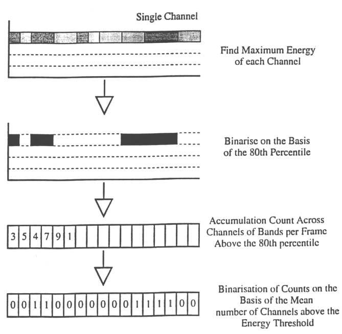
Schematic summary of the steps involved in fragmenting the speech into energy and silence. The depiction in the top section is in conventional spectrogram format: Time is plotted along the abscissa, frequency along the ordinate, and energy is represented on a grey scale. The steps in computation in the top two sections are shown for a single frequency band of the vocoder outputs.

From these patterns for the ATE “energy” sections three measures were obtained: how fragmentary these sounds were (number of regions), their length (mean duration), and how variable they were (SD). The same three parameters were obtained for the BTE “silent” sections, which gave six parameters in total for the fragmentation group. All these parameters might help separate Rs and Ps to the extent that the energy and silence in Rs are more regularly spaced in time than the apparent fragmentations in Ps. Thus, these statistics may aid the ANN to learn to differentiate an R fragmentation pattern like that shown in Figure 1 from a spurious fragmentation that appears at word onset in a P as shown in Figure 2.

The initial conception behind the development of spectral parameters was to offer a measure of the stability of the spectrum across the word. It was expected that Rs and Ps would show more spectral stability than fluent words as they are produced with a relatively stable vocal tract configuration. It was necessary that the parameter that reflected this “stable pattern” was not restricted to looking for peaks in specific frequency regions. That would have been tantamount to having a phone detector, which would have entailed a more detailed level of processing. The constraint this requirement imposed on the spectral metric was that it had to reflect spectral stability across repeated or prolonged phones with very different spectral composition (e.g., fricatives vs. nasals).

It is also pertinent at this point to recall that the speech has been divided into ATE and BTE regions since spectral similarities are expected to be related to these: If an R is considered and the fragmentation computation has separated ATE from BTE sections, the spectrum of the ATE sections would be similar (ameliorated to some extent by transitional and durational smearing). A similar situation would apply to BTE regions. However, ATE spectra would be expected to differ from BTE spectra since the spectrum of silence differs from the spectrum of energy-filled sections. For a P that is all ATE, the spectrum should be stable throughout. If the P has been fragmented as happens in the example in Figure 3, the ATE and BTE sections when considered separately would have similar spectra, but ATE and BTE should be more similar than in Rs. (The overall level will be lower in BTE sections than ATE sections; otherwise they would have been designated ATE.) Thus, these parameters might also allow the ANN to detect apparent fragmentations in Ps. These considerations stress the need for having coefficients that provide a measure of spectral similarity across ATEs alone, across BTEs alone, and across adjacent ATEs and BTEs. For an F word, ATE sections will have different spectra though BTE sections would have similar spectra for silences located within the word.

The first step in spectral processing applied to each separate ATE and BTE section was to average the spectrum over all adjacent nonoverlapping 10 ms frames that occurred within either the ATE or the BTE region. The averaging applied to the signals in these regions accentuated any veridical peaks in the spectral pattern. Comparisons were next made over adjacent occurrences of the three different types of region (ATE to next ATE, BTE to next BTE, ATE to adjacent BTE). The processing applied to these three types of region was the same and is described for ATE-ATE types. First, the mean energy over all 19 frequency bands was calculated over the entire duration separately for each ATE section. All adjacent ATE sections were taken starting with the first and second sections. The member of each pair that had the lowest mean energy was then scaled by a constant so that it had the same maximum value as the one with the higher mean. This was done to remove energy differences. Next, the spectrum of the second section was inverted and added to the first one. This reduced the two sets of 19 coefficients to one set. If the spectra had peaks in the same frequency regions, inverting and adding the spectra would produce a flat spectrum (i.e., the peaks in one spectrum are removed due to the inversion converting them to troughs). Finally, the SD of the 19 coefficients was taken: If the spectra were the same, the SD would be small, but if the spectra were different, the SD would be large. In words fragmented into several parts, the SD of each consecutive pair was obtained as described and the average of this value obtained. In Figure 4, the steps involved in obtaining the SD are summarized in schematic form, and the patterns expected in the SDs are summarized in Table 1 for Ps, Rs, and Fs. Table 1 shows that the pattern in this measure should separate the P, R, and F words. Note, in particular, that spectral stability throughout a word (as in Ps) shows low values for these parameters for comparison of all section pairs.

Figure 4.

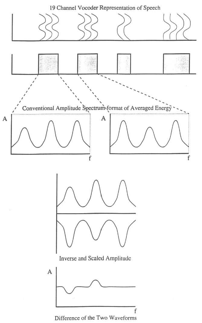
Schematic summary of the steps involved in computing spectral measures between ATE sections for a repetition. The spectra in successive 10 ms frames are shown at the top: Time is along the abscissa, frequency along the ordinate, and the solid line indicates relative energy. The location of ATE (shaded) and BTE (white) regions (obtained in the way summarized in Figure 3) are indicated in the section beneath. The averaged spectra for the first and second ATE regions are depicted on the left and right of the third panel in standard amplitude spectrum-format. The amplitude spectrum of the first ATE region and the scaled and inverted second spectrum are next shown on the same axes. The differenced waveforms are shown in the final section. The SD across all 19 spectral coefficients is taken. The steps involved in computing spectral measures between BTE sections and across adjacent ATE and BTE sections is similar.

Table 1.

Expected pattern of standard deviation of spectrum parameters across ATE and BTE sections for Ps, Rs, and Fs. The calculation of the standard deviation measure is described fully in the text and is summarized in Figure 4.

	ATE-ATE	BTE-BTE	ATE-BTE
Reps	low	low	high
Pros	low	low	low
Flu	high	low	high

Part-Word Parameters

It has been stressed that the properties of Rs and Ps are word-position dependent. Consequently, the next parameters separated activity in the first part of a word, where stuttering was likely to occur (Wingate, 1988), from the remaining activity within a word, that, conversely, was far less likely to contain evidence of stuttering. Simply dividing the word into two halves along the time base was not adequate for Rs, words that started with pauses, and Ps on low intensity sounds. These sometimes had sections of low energy that lasted a long time compared with the fluent word that was ultimately spoken. In such circumstances, both the first and second half of the word might have included silent sections or long sections that had low energy. To ensure that the word was subdivided sensibly when energy was skewed to the final part of a word, as occurred in these situations, the word was split into two sections based on an energy criterion: The energy within each 10 ms time frame was first cumulated across all spectral bands and then these were cumulated across all time frames. The point in time at which the cumulated energy across time frames reached half its final value was then obtained and the point in time at which this occurred was used to divide the word into its first and second parts. Since the duration of the first and second parts might show whether the word contains an R or P, the two durations were included as a group of parameters to investigate. This processing was done irrespective of the number of syllables in the word (recall, however, that 90% of the words are monosyllabic).

The energy might show different fluctuations in the first part (a relatively high number of fluctuations in the first part of an R, few in a P, compared in each case with the first part of an F word). Besides these potential bases of comparison between first parts, the parameters might also reveal differences between dysfluency categories by providing separate information about the first and second parts within a word of each type: Only the first and second parts of an F word are themselves F. Consequently, differences in the energy parameters (or, for that matter, any parameters) between first and second parts of a word, potentially provide further information about the category of the word. Again, the complex relationship between parameters supports use of ANNs as appropriate for learning such mappings between input parameters and event classifications. The energy group of part words had two parameters: the SD of energy in the first and second parts.

The fragmentation parameters seen in Rs and to some extent in Ps already described for whole words should be dominant in the first part and the remaining part should be much like the pattern seen in a fluent word. Fluent words should have more similar fragmentation patterns in both parts. Thus, subdivision of the word should serve to clarify the fragmentary pattern in the first part, and these parameters should exhibit a different pattern from the second part. Consequently, the six fragmentation parameters described in connection with whole words were included separately for the first and second parts (12 parameters in total).

In the light of the earlier observation that Rs and Ps tended to occur at the beginning of a word, the averaged spectra should have more marked spectral peaks at the onset of R or P words than at the end (see the second row of Figures 1 and 2). Fluent words will have less marked spectral peaks throughout. After the processing depicted in Figure 3 was done for each part, there were six spectral parameters in all.

Two final points to note about choice of these parameters are that they should be to some extent immune from noise and that it should not be necessary to have the word boundaries located in exactly the same positions as those of the human judges. The partial noise immunity is because both the fragmentation and spectral parameters involve computations applied to all 19 separate frequency bands. Thus, if a band-limited room noise occurs, it will affect specific frequency regions. This would leave the pattern structure that the computations attempt to elucidate to be established in the unaffected bands. The robustness with respect to word boundary positioning arises because the parameters do not reflect transient features but a property of regions of speech.

All the parameter groups and the separate parameters within each group are summarized in Table 2. Not all the input parameters will necessarily be needed to achieve good ANN recognition due, for instance, to redundancy between them. All combinations of parameter groups are trained and each of these combinations specifies a unique set of inputs that, in turn, specifies a different ANN. The architecture of each of these ANNs is the same and a description of this is given next.

Table 2.

Summary of parameter groups (I-IX). The number of separate parameters in each group are indicated in parentheses.

Whole word measures

I. Duration of word (one parameter) II. Fragmentation measures: Number of energy peaks, mean duration and SD. The same parameters are also obtained for silent sections (six parameters in all). III. Spectral measures for whole word. SD between ATE sections, between BTE sections and between adjacent ATE and BTE sections (three parameters).

Measures for first and second part of words

IV. Duration of first and second parts (two parameters) V. SD of energy in first and second parts as a measure of fluctuation (two parameters). VI and VII. Part-word fragmentation measures: Peak count parameters for first and second parts as obtained for the whole word (6 parameters per part making 12 in all). VIII and IX. Part-word spectral measures as obtained for the whole word (three parameters per part making six in all).

Total number of parameters per word = 32

ANN Architecture

The networks attempt to associate input parameters selected from one or more of the groups shown in Table 2 onto one of the three category responses: P, and R, and, by default if there was no evidence for either D category, F. Separate networks were trained using parameters from words selected in the manner described earlier from all 6 training-set children who stutter.

Each ANN was trained using Fahlman and Lebiere's (1990) Cascade Correlation (CC) procedure. A schematic showing how an ANN is built up using this algorithm is given in Figure 5. CC is a constructive meta-algorithm in which other algorithms such as back propagation (BP) are embedded. Learning takes place by repeating two steps. The top section of Figure 5 shows the initial state of the ANN prior to training. The horizontal lines indicate unit outputs and the vertical lines unit inputs. As shown, all input units are connected to all output units and this remains true throughout training. At this stage there are no hidden units so all the weights are trainable.

Figure 5.

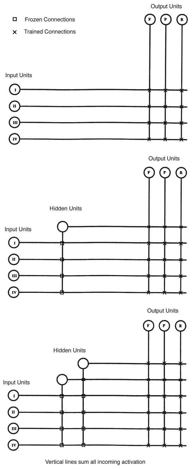
Buildup of the architecture using cascade correlation for an ANN with four inputs. Inputs are shown on the left (groups are indicated by the Roman numeral and these are detailed fully in Table 2). F, P, and R output units are indicated at the top. Hidden units are added going from the top (no hidden units) to bottom (three hidden units) of the figure as described in the text.

The first phase in the algorithm proper is nonconstructive and uses the embedded standard learning algorithm, which was BP here. During this phase the ideal activity as specified in the training pattern is compared with the actual activity and the weights of all trainable connections adjusted to bring these into correspondence. This is repeated until learning ceases or a predefined number of cycles has been exceeded. For the initial network there are no fixed connections as no hidden units have been added so all connections are trained. However, it is important to note that processing proceeds in the same manner when there are hidden units (as there will be when this step is repeated during later iterations).

The second phase is constructive and involves the creation of a pool of “candidate” units (in our case, eight). Each candidate unit is connected with all input units and all existing hidden units. (When hidden unit connections exist on later iterations, they are being treated the same as input units by the candidate units.) At this stage, there are no connections to the output units. The links leading to each candidate unit are trained by the selected standard learning algorithm (BP here) to maximize the correlation between the residual error of the ANN and the activation of the candidate units. Training is stopped if the correlation ceases to improve or a predefined number of cycles is exceeded. The final step of the second phase is the inclusion, as a hidden unit, of the candidate unit whose correlation was highest. This involves freezing all incoming weights (no further modifications will be made and those connections will be untrainable) and creating randomly initialized connections from the selected unit to the output units. The new hidden unit represents, as a consequence of its frozen input connections, a permanent feature detector. The weights from this new unit and the output units are trained. Since the outgoing connections of this new unit are subject to modification, its relevance to the final behavior of the trained ANN is not fixed. The unselected candidate units are destroyed. The resulting ANNs, when the first and second hidden units have been added in, are shown, respectively, in the middle and bottom sections of Figure 5. The two phases are repeated until either the training patterns have been learned to a predefined level of acceptance or a preset maximum number of hidden units have been added, whichever occurs first. The algorithm is implemented in the Stuttgart Neural Network System and this package was employed for constructing the current ANNs.

During testing, all the words from the 6 test speakers were classified irrespective of flow rating, including words that were parts of supralexical and O dysfluency classes. The words that the supralexical parser indicated were parts of repairs or the words that the judge had said were O dysfluencies were excluded during statistical analysis.

Results

ANNs were deemed to have classified a word correctly if they assigned it to the same category as the judge whose categorizations were used for training the networks. For all ANNs, overall accuracy was computed as the percentage of words classified correctly out of all the words irrespective of the particular category designation (F, P, or R) of the word. The ANNs were rank ordered in terms of the overall percentage correct and these are presented in Table 3 for the 10 best ANNs. The parameter groups involved in each ANN are indicated in the first column (the Roman numerals correspond with those in Table 2). It can be seen that the best 10 networks had overall accuracy ranging between 92.00% and 90.90%. Thirty-three of the ANNs classified more than 90% of all words correctly.

Table 3.

Results for the 10 best ANNs for classifying words overall. The parameter groups incorporated in each ANN can be identified by the Roman numeral by reference to Table 2. The percentages of F words correctly classified out of the total F words are given in the next column. The percentages of P and R words are presented in the same manner in columns three and four. Ps and Rs collapsed into a gross D category are given as the percentage correctly classified in column six (computed in the same manner as before). In the final column, the percentage of words classified correctly into either F, P, or R categories out of the total words is given (the percentages in this column are the basis for rank ordering the ANNs). All category designations used for scoring these results are from the most experienced judge. A breakdown of parameter groups for the best 10 ANNs is given at the floor of the table. This is a count of how many ANNs the designated parameter group featured in the best 10 ANNs

	Percentage
Parameters	F	P	R	D	Overall
II, III, IV, V	95.07	58.14	42.86	78.01	92.00
IV, V, IX	95.60	44.19	28.57	74.47	91.59
IV, V, VI, VII	94.87	53.49	36.73	76.60	91.45
IV, VI, IX	94.19	53.49	51.02	80.14	91.45
II, IV, V, VI	93.89	55.81	53.06	80.85	91.32
I, IV, VI	94.09	46.51	47.96	79.43	91.09
I, II, IV, V, VI	93.89	62.79	43.88	78.72	91.04
IV, V	94.97	39.53	31.63	78.72	91.04
II, V, VI, VII, VIII	93.31	62.79	53.06	80.85	90.90
IV, V, VII	94.82	32.56	34.69	76.60	90.90
IV	V	VI	II	VII	IX
9/10	8/10	6/10	4/10	3/10	2/10
I	III	VIII
2/10	1/10	1/10

The first factor of note is that all the ANNs employed at least three parameter groups. Thus, no single parameter alone was satisfactory for categorization of R and P. Comparison over ANNs shows that only three parameter groups were involved in 5 or more out of the 10 best ANNs (IV, V, and VI). All of these 10 ANNs had at least one of these parameter groups. However, it cannot be concluded that these three parameter groups are best at doing the classification: To assess the role of parameter group IV, the sixth-best ANN had parameter groups IV and VI that were involved in five or more of the best 10 ANNs and classified 91.09% correct. The ninth ANN did not have IV (it had V and VI of the parameters involved in five or more of the best 10 ANNs) but classified only 0.19% fewer words correctly overall. Second, the ANN involving parameter groups IV, V, and VI was 18th overall (not shown) with 90.40% classified correctly overall. These observations underline the fact that the complex relationship between the parameters is what determines performance, which is why ANNs are needed for this task.

The proportion of F words was computed as the percentage of F words correctly classified out of all F words and these are presented in column two of Table 3. The corresponding percentages for P and R are given in columns three and four. F classification is above 93% for all of the 10 best ANNs. However, the majority of ANNs for locating P and R are somewhat disappointing at around 50%.

The reasons for this may be that Ps and Rs are confused either with themselves or, more seriously, with Fs. To assess which of these obtained, Ps and Rs were both scored as a grosser dysfluent category (D). Percentage of D words correctly classified out of all D words are given in the fifth column of Table 3. It can be seen that accuracy of this grosser category jumps to 78.01% for the best ANN and is also around 80% for the other nine best ANNs. Thus, it appears that inter-dysfluency classification errors (i.e., between Ps and Rs) are prevalent. Consequently, the principle limitation in these ANNs is that there is some confusion between Ps and Rs. Some similar features occur in the human categorization data in Howell et al. (1997). Perusal of the 4 and 5 flow ratings in Table 3 of Howell et al. show that of the 14 nonagreed-upon categorizations of P and R, 8 involved P/R confusions, and only 6 involved P or R confusions with an F production. This may suggest that humans also confuse these types of D. The P/R confusions are, however, at a lower rate than observed here. It may be, therefore, that humans are sensitized to look for continuity in sounds that show spectral continuity even when they are interrupted briefly (Bregman, 1990). Consequently, they may miss subtle fragmentations in Rs and Ps leading to inter-dysfluency class confusions. Alternatively, the input parameters to the ANNs may need improving (principally, the spectral similarity parameters that are relatively crude).

Discussion

The ANNs whose performance has been reported in this paper were trained and tested on human judgment data reported in Howell et al. (1997). High levels of agreement are a prerequisite before attempting to train and test ANNs to separate F, P, and R. In this connection, some features of the data of Howell et al. (1997) had a bearing on selection of training material for the ANNs. Flow ratings were obtained from human judges besides each word's categorization. The data showed Rs exhibited good agreement across all D rating-values (3-5) but Ps were more variable (due to variability across judges in making duration judgments). Accuracy of Ps was, however, 80% for words given flow rating 4 and 5. For this reason, in the current study, only words given 4 or 5 flow ratings for P instances were used for training material. An equal number of R words given these same flow ratings and Fs given flow ratings of 1 were selected for training the ANNs. All words in the test set of speakers, irrespective of their flow rating, were used for assessing ANNs.

Two components of a fully automated system have not been addressed in this study. First, SD were processed out with a computer-parser that works on supplied transcriptions. Future possible ways of automating this step that will be explored are to locate these structures by looking for patterns of repeated words and using the distinctive prosodic properties of SD (see Howell, Kadi-Hanifi, & Young [1990] for details of the prosody of SD, and Howell & Young [1991] and Levelt & Cutler [1983] for details of the prosody of related structures produced by fluent speakers).

Second, word segmentations were supplied from human judgmental data (Howell et al., 1997). In the same way as for SDs, a fully automated procedure will require the word markers to be computed. Initial results have been reported for words employing a dynamic time-warping algorithm (Howell, Sackin, Glenn, & Au-Yeung, in press). Considerable progress has been made on automatic syllabification by other workers who have been examining fluent speech (Hunt, 1993; Kortekaas, Hermes, & Meyer, 1996) and by ourselves with stuttered speech. Using syllables has the advantage that it can be applied to spontaneous speech (see Howell et al. [1997] for a discussion of this topic). Since automatic syllable segmentation looks promising, the classification difficulty has not simply been shifted to a problem of segmentation. A further point to note is that pre-segmentation of speech represents a new approach to the problem of dealing with time variation when categorizing serially arrayed events (like speech). Once word or syllable segments have been located, a fixed number of parameters can be obtained to categorize variable-length speech segments. Time variation is a particularly acute problem when dealing with stutterings as they can vary in duration to a greater extent than do other speech sound classes such as phones.

A set of pattern parameters was next developed from definitions of the acoustic patterns that characterize Ps and Rs. The parameter groupings involve duration, energy, energy fragmentation, and spectral similarity, with parameters computed for whole and part words where applicable. Particular attention was given to ensuring these do not require exact boundary location and that they show some noise immunity. ANNs were trained and tested with all possible parameter-group combinations. The best network (in the sense of obtaining good separation of F from D categories and acceptable division of the D category into P and R) involved (a) measures of the energy-silence fragmentation parameter over all the word (II), (b) spectral comparison measures across ATE-ATE, BTE-BTE, and ATE-BTE regions (III), (c) part-word duration (IV), and (d) energy variability within each part of a word (V).

Earlier in this discussion, it was stated that once the automatic procedure has been evaluated it could serve as a benchmark standard for assessing stuttering and the way it changes. Follow-up data from (a) a London clinic and (b) using an experimental procedure involving hypnosis are being investigated using this procedure, with promising results. It is notable that the recordings from the London clinic were not made in a studio environment and the system still operated well. Thus, the argument that these procedures should be to some extent noise immune seems to be empirically verified.

Finally, although the prototype system works, this does not mean that no improvements and extensions are envisaged. Some of the main areas for future research are:

1. Investigation of alternative architectures. For example, a hybrid architecture could have as its first step an F/D detector followed by differentiation of Ds into Rs and Ps.

2. It is possible that more training data would improve the performance. Also, different ways of constructing the training sets need to be explored.

3. The input parameters would almost certainly benefit from further work. Nevertheless, though the parameters that have been developed might be improved, they provide a sufficient basis for exploring the ANNs. Also, any improvements are more likely to be found in the parameterization rather than the basic groupings that have been used.

4. Extension to wider populations of children who stutter, principally younger children with more variation in severity and with different native languages.

References

- Abercrombie D. English phonetic texts. London: Faber and Faber; 1964. [Google Scholar]
- Bregman AS. Auditory scene analysis: The perceptual organisation of sound. Cambridge, MA: MIT Press; 1990. [Google Scholar]
- Brown SF. The loci of stutterings in the speech sequence. Journal of Speech Disorders. 1945;10:181–192. [Google Scholar]
- Elman JL, Zipser D. Learning the hidden structure of speech. Journal of the Acoustical Society of America. 1988;83:1615–1626. doi: 10.1121/1.395916. [DOI] [PubMed] [Google Scholar]
- Fahlman SE, Lebiere C. The cascade-correlation learning architecture. Pittsburgh, PA: Carnegie Mellon University, Department of Computer Science; 1990. (Tech. Rep. No. CMU-CS-90-100). [Google Scholar]
- Holmes JN. Speech synthesis and recognition. London: Chapman and Hall; 1992. [Google Scholar]
- Howell P. Syllabic and phonemic representations for shortterm memory of speech stimuli. Perception and Psychophysics. 1978;24:496–500. doi: 10.3758/bf03198773. [DOI] [PubMed] [Google Scholar]
- Howell P, Hamilton A, Kyriacopoulos A. Speech Input/Output: Techniques and Applications. London: IEE Publications; 1986. Automatic detection of repetitions and prolongations in stuttered speech. [Google Scholar]
- Howell P, Kadi-Hanifi K, Young K. Phrase repetitions in fluent and stuttering children. In: Peters HFM, Hulstijn W, Starkweather CW, editors. Speech motor control and stuttering. New York: Elsevier; 1990. pp. 415–422. [Google Scholar]
- Howell P, Sackin S, Glenn K. Development of a two-stage procedure for the automatic recognition of dysfluencies in the speech of children who stutter: I. Psychometric procedures appropriate for selection of training material for lexical dysfluency classifiers. Journal of Speech, Language, and Hearing Research. 1997;40:1073–1084. doi: 10.1044/jslhr.4005.1073. [DOI] [PMC free article] [PubMed] [Google Scholar]
- Howell P, Sackin S, Glenn K, Au-Yeung J. Automatic stuttering frequency counts. In: Peters HFM, Hulstijn W, van Lieshout P, editors. Speech motor control and stuttering. New York: Elsevier; in press. [Google Scholar]
- Howell P, Young K. The use of prosody in highlighting alterations in repairs from unrestricted speech. Quarterly Journal of Experimental Psychology. 1991;43A:733–758. doi: 10.1080/14640749108400994. [DOI] [PubMed] [Google Scholar]
- Hunt A. Recurrent neural networks for syllabification. Speech Communication. 1993;13:323–332. [Google Scholar]
- Johnson W, Boehlmer RM, Dahlstrom WG, Darley FL, Goodstein LD, Kools JA, Neeley JN, Prather WF, Sherman D, Thurman CG, Trotter WD, Williams D, Young M. The onset of stuttering. Minneapolis: University of Minnesota Press; 1959. [Google Scholar]
- Jordan MI. Serial order: A parallel distributed approach. San Diego, CA: University of California at San Diego, Institute for Cognitive Science; 1986. (ICI Report 8604). [Google Scholar]
- Kortekaas RWL, Hermes DJ, Meyer GF. Vowel-onset detection by vowel-strength measurement, cochlear-nucleus stimulation, and multilayer perceptrons. Journal of the Acoustical Society of America. 1996;99:1185–1198. doi: 10.1121/1.414671. [DOI] [PubMed] [Google Scholar]
- Levelt WJM, Cutler A. Prosodic marking in speech repair. Journal of Semantics. 1983;2:205–217. [Google Scholar]
- Rumelhart F, McClelland JL. Parallel distributed processing: Explorations in the microstructure of cognition: Vol 1, Foundations. Cambridge, MA: MIT Press; 1986. [Google Scholar]
- Sackin S, Howell P. A two-stage strategy for the automatic recognition of dysfluencies in child stutterers' speech: III. ANN syllable segmentation of spontaneous speech. In preparation. [Google Scholar]
- Starkweather CW, Gottwald SR, Halfond MM. Stuttering prevention: A clinical method. Englewood Cliffs, NJ: Prentice-Hall; 1990. [Google Scholar]
- Sweet H. A primer of spoken English. Oxford: Clarendon Press; 1895. [Google Scholar]
- Wingate ME. The structure of stuttering: A psycholinguistic study. New York: Springer-Verlag; 1988. [Google Scholar]