Automated Neurite Extraction Using Dynamic Programming for High-Throughput Screening of Neuron-Based Assays

Abstract

High throughput screening (HTS) of cell-based assays has recently emerged as an important tool of drug discovery. The analysis and modeling of HTS microscopy neuron images, however, is particularly challenging. In this paper we present a novel algorithm for extraction and quantification of neurite segments from HTS neuron images. The algorithm is designed to be able to detect and link neurites even with complex neuronal structures and of poor imaging quality. Our proposed algorithm automatically detects initial seed points on a set of grid lines and estimates the ending points of the neurite by iteratively tracing the centerline points along the line path representing the neurite segment. The live-wire method is then applied to link the seed points and the corresponding ending points using dynamic programming techniques, thus enabling the extraction of the centerlines of the neurite segments accurately and robustly against noise, discontinuity, and other image artifacts. A fast implementation of our algorithm using dynamic programming is also provided in the paper. Any thin neurite and its segments with low intensity contrast can be well preserved by detecting the starting and ending points of the neurite. All these properties make the proposed algorithm attractive for high-throughput screening of neuron-based assays.

1. Introduction

Knowledge and tools from cellular and molecular biology is playing an increasingly important role in assisting researchers in the pharmaceutical industry in studying the mechanisms of diseases and in finding better drug hits and leads. High-throughput screening (HTS) technology has recently emerged as an important drug discovery tool for identification of biological probes and drug leads by screening large volume, diverse biochemical and cell-based assays (Feng, 2002, Cacace et al., 2003, Dunkle, 2003, Fox, 2003, Gaunitz and Heise, 2003, Klyushnichenko, 2003, Yarrow et al., 2003, Perlman et al., 2004). The power of the high-throughput screening comes from the automated fluorescence microscopy imaging techniques that make it possible and facile to visualize the complex biological processes at the cellular and molecular levels and allow speedy and economic acquisition of such high throughput neuron image data. This technology generates huge amounts of fluorescence microscopy images, with each image containing several million pixels. Accessing these data to extract and compose useful information requires efficient and cost-effective image analysis tools that involve minimum human interaction, the image processing task of which has been a challenging problem for years.

In the context of high-throughput screening of neuron-based assays, the fundamental goals of neuron image processing include: 1) measuring the length of the total neurite segments, and 2) detecting and segmenting neuron cells. In this paper, we consider the problem of automatically extracting and labeling all the neurite segments in a fluorescence microscopy neuron image. We observe that an individual neurite segment can be treated as a bright elongated wire-like structure surrounded by dark background; in this way, the problem is equivalent to the problem of extracting line structures from digital images.

The existing research work on extraction of line structures in digital images can be roughly categorized into three groups. The first group of algorithms is generally referred to as tracing-based algorithms (Collorec and Coatrieux, 1988, Coatrieux et al., 1994, Janssen and Vossepoel, 1997, Polli and Valli, 1997, Can et al., 1999, Al-Kofahi et al., 2002, Al-Kofahi et al., 2003). When extracting a single neurite segment, these algorithms start from an automatically selected seed point and detect a series of points along the centerline of the segment by estimating the local direction of each point. Each centerline point is traced based on its previous detected centerline point in a recursive manner until certain stopping conditions are satisfied. This group of algorithms is efficient since it only processes the pixels that are close to the line structures. Another advantage is that no further linking algorithm is needed since the points on the neurite segment can be linked and labeled during the tracing process. However, since most of these algorithms consider only the grayscale values and their estimation of the local directions is not robust, their performance on line extraction is quite low for images with poor quality or of complex line structures.

The second group of algorithms on line extraction is based on the concept of line-pixel detection (Chaudhuri et al., 1989, Wang and Pavlidis, 1993b, a, Kweon and Kanade, 1994, Maintz et al., 1996, Steger, 1996, Sato et al., 1998, Steger, 1998, Frangi et al., 1999, Wink et al., 2002). For each pixel, the algorithms consider local geometric properties of the lines, such as ridges and ravines, as well as their local orientations. The line pixels can be extracted accurately by modeling the 2-D line profiles and examining its first and second derivatives using the Gaussian smoothing kernel (Florack et al., 1992, Iverson and Zucker, 1995, Lindeberg, 1998). After detecting all the individual line pixels, additional effort is needed to link them together (Steger, 1998). Although highly precise on extracting lines, these algorithms suffer a drawback that thin lines or lines with low intensity contrast may be smoothened out unintentionally by the Gaussian kernel, resulting in the loss of the corresponding neurite segments. Furthermore, they cannot resolve issues of discontinuities since there are no line pixels found in the breaking areas.

The third group is searching-based algorithms (Barrett and Mortensen, 1996, Falcão et al., 1998, Mortensen and Barrett, 1998, Falcão et al., 2000, Meijering et al., 2004). Given each pair of starting point and ending point, these algorithms extract the line by searching for an optimal path from the starting point to the ending point. An optimal path can be found by calculating the globally minimal cumulative cost using a predefined cost function (Meijering et al., 2004). This is also referred to as live wire algorithm based on dynamic programming technology. Although robust against noise and discontinuities in line structures, these algorithms are unable to extract a line when a starting point is located within a large bright region with intensity values evenly distributed (usually a region of neuron cell body). They are computationally expensive since they search for and find an optimal path for every pixel in the image, not only for the ending point. The requirement of manually selecting starting points and ending points makes it certainly impractical for high throughput screening applications.

Based on the aforementioned observations and increasing development of high-throughput screening of neuron-based assays, we believe that it is necessary to develop an automated image analysis algorithm to extract and label the neurite segments accurately and completely with minimum user intervention. In this paper, we propose a novel algorithm for automatic labeling and tracing of neurite segments in microscopy neuron images. The algorithm selects the starting and ending points automatically and links the line using dynamic programming techniques. Sections 2 and 3 describe the automatic selection of starting points and ending points while the linking algorithm using dynamic programming is presented in Section 4. Section 5 shows the experimental results and the validation method used to verify the extraction performance. The selection of the parameters and their effect on performance are also discussed. Section 6 presents our conclusions.

2. Starting point selection

We present in Fig. 1 a block diagram for our proposed algorithm. The input images are pre-processed to remove undesirable features and enhance branching structures. The starting points and the ending points of the neurite segments can be automatically detected so that human interaction is no longer required. The points are then linked automatically using dynamic programming technique. Each step is discussed in detail in the following subsections.

Fig. 1.

The block diagram for the neurite tracing algorithm using dynamic programming

A starting point, also called a seed point, is a point on or near the centerline of a neurite segment. To extract all the neurite segments, at least one starting point should be selected on each individual segment. More than one starting point is needed in cases where the neurite structure is complex or the intensity contrast is very low along the neurite segment.

When selecting the starting points, only N horizontal lines and M vertical lines in the neuron image are considered. The pixels on each of the horizontal or vertical lines are first processed by a low-pass filter in the form of [0.25 0.5 0.25]^T, an approximation of the 1-D Gaussian kernel. Since a discrete approximation in this form involves only local fixed point shifting and adding operations, the computational cost for the convolution can be significantly reduced. Thus, high-frequency components are removed from the sequence of pixels. After low-pass filtering, local intensity maxima are searched and detected using a window of size W along each line. W should be chosen so that at least one maximum is detected on each neurite segment. Thus, a small value is desired. In our work, we use the minimum expected neurite width as the value for W. Such a small window size may leads to multiple local maxima at locations where the neurite segments are very wide. This is how redundant seed points are detected. We believe that it is necessary to use redundant seed points so that the extraction is complete, partially because our targeted neuron images have very complicated neurite structures. The starting points will be selected among the local maxima detected on the set of grid lines.

We select the starting points based on the following two criteria:

• Criterion 1: the local maxima I_m has an intensity value that is larger than or equal to a threshold value T_I: I_m≥T_I.

• The threshold value is determined by the intensity values of the image: T_I=μ_I+σ_μ, where μ_I is the median intensity value of all the pixels, and σ_μ is the standard deviation calculated based on μ_I. This way, we pick up the pixels having intensity values that are above the average intensity of the image. However, those pixels whose intensity values are below the averaged intensity value and are on or near neurite segments will be ignored. Thus we need the second criterion for these pixels.

• Criterion 2: the local maximum, I_m, has a local signal-to-noise ratio, SNR_m, that is larger than or equal to a threshold value T_SNR: SNR_m≥T_SNR.

• SNR_m is calculated based on the point m and its local neighborhoods N_m, a 10 ×10 block of pixels centered at the point m. We calculate a local threshold value T_N for the neighborhoods N_m using Otsu’s algorithm (Otsu, 1979). The pixels in N_m are grouped as the foreground if their intensity values are larger than or equal to T_N. The rest of the pixels in N_m are then grouped as the background. By defining the mean value of the intensities of the foreground pixels and background pixels as μ_f and μ_b respectively, and the standard deviation of the background pixels as σ_b, the local signal-to-noise ratio SNR_m is calculated as follows:

  $${\mathit{SNR}}_m=\frac{{\mu }_f-{\mu }_b}{{\sigma }_b}$$ (1)

  the threshold value T_SNR is determined by the mean value of all the local signal-to-noiseratio calculated by (1) for all the local maximum point m detected previously:

  $$T_{\mathit{SNR}}\ge \underset{m}{\mathit{median}}\left\{{\mathit{SNR}}_m\right\}$$ (2)

  In other words, if a local maximum point has an intensity value that is below the threshold, we still keep it as a starting point if its local SNR is above the average SNRs among all the local maxima points.

3. Ending point selection

An ending point is identified by iteratively tracing a single neurite segment from the selected starting point until the end of the segment. The track does not need to be accurate or smooth; since the accuracy and smoothness of the track will be achieved by the linking process based on dynamic programming technique. Thus we need to design a rapid but rough tracing method which has robust stopping criteria for selection of the ending points. A tracing from the current point p_i to the next point p_i+1 can be described as estimating the local direction d_i for p_i, and tracing along d_i to find the point p_i+1. The tracing starts at one of the starting points, steps forward from one point to another along the neurite segment, and stops when the stopping conditions are satisfied, at which the ending point is identified. The question is then how to estimate the local direction of a pixel in the image.

The local direction d_i of point p_i is estimated by correlating the neighborhoods of p_iwith a set of 2-D directional correlation patterns. Early usage of such directional correlation patterns can be found in (Sun et al., 1995) and later they were widely used in (Can et al., 1999, Al-Kofahi et al., 2002). A correlation pattern, also called a template, is defined as a 2-D filter that calculates a low-pass differential perpendicular to the direction of a line and low-pass averaging along the direction of the line. An example of such patterns, designed to calculate the correlation along the x-axis direction (0° direction), is shown in Fig. 2. Obviously a point on a line structure along the x-axis direction will have the maximum correlation with such a pattern among all the 2-D directions that a line structure could have. The patterns at other directions can be generated by rotating the one at 0° direction. Notice that the first two lines of the pattern in the figure have opposite signs compared to the last two lines of the pattern. This means that the maximum correlation occurs at the boundary of the line structure. Thus the local direction of a centerline point can be estimated by correlating the corresponding points on or near the edge of the line structure, which is achieved by searching for the edge points along the two directions perpendicular to the local direction.

Fig. 2.

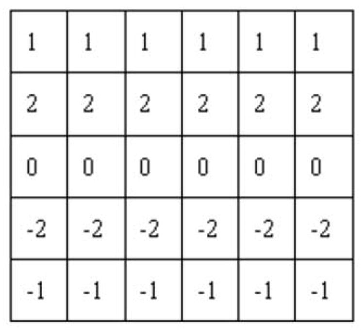
The correlation kernel at 0° direction.

Since the local direction is unknown, we need to do searching for all the possible 2-D directions. To simplify the process, all the 2-D directions are quantized into 16 directions (Can et al., 1999), each represented by an integer number. We denote the quantized direction as d^k where k = 0,1,…15. There exists a pair of patterns for each d^k, one for the left edge and the other for the right edge. They are denoted as $T_L^k$, $T_R^k$, with subscripts L,R indicating the direction toward the left edge or the right edge. The two directions perpendicular to d^k are denoted as $d_L^k$ and $d_R^k$. The correlation g between the patterns $T_L^k$, $T_R^k$ and a point p_i with the coordinate (m,n) is calculated as follows:

$$\begin{array}{l}{g}_L^k(m,n)=\sum _{x,y}{N}_p(m+x,n+y)\ast T_L^k(x,y)\\ g_R^k(m,n)=\sum _{x,y}{N}_p(m+x,n+y)\ast T_R^k(x,y)\end{array}$$ (3)

where N_p is the neighborhoods of p_i selected as a 5×6 block of pixels with p centered at the leftmost column. “*” denotes the multiplication operator. Such a correlation operation obviously indicates the “matchness” between the pattern and the image at each point. For each left direction $d_L^k$ and its pattern $T_L^k$, we search for a maximum correlation calculated by (3) beginning from p_i until a pre-defined maximum possible width W_max, resulting in a total of 16 such maximum correlations. The highest correlation represents the best match and thus the corresponding direction can be selected as the estimation of the local direction. The same search is also applied along the right direction $d_R^k$. The highest correlations are obtained as follows:

$$\begin{array}{l}{G}_L=\underset{k,(m,n)}{\max }\{g_L^k(m,n)\}\\ G_R=\underset{k,(m,n)}{\max }\{g_R^k(m,n)\}\end{array}$$ (4)

where G_L,G_R denotes the highest correlations along the left and right directions respectively. The points at which the highest correlations occur are identified as the edge points and are denoted as p_L,p_R:

$$\begin{array}{l}{p}_L=(m_L,n_L)=\underset{k,(m,n)}{\text{arg max}}\{g_L^k(m,n)\}\\ p_R=(m_R,n_R)=\underset{k,(m,n)}{\text{arg max}}\{g_R^k(m,n)\}\end{array}$$ (5)

since the current point p_i may not be on or near the centerline, its location needs to be adjusted. The new location of p_i resides at the middle point of the line between p_L andp_R. The local direction for p_i is estimated as the direction whose correlation is the highest in a total of 32 maximum correlations:

$$d_i=\underset{k}{\text{arg max}}\{G_L,G_R\}$$ (6)

The next point p_i+1 is traced from p_i along the direction d_i as follows:

$$p_{i+1}=p_i+d_i$$ (7)

Once the local direction of a point is determined, the local direction for the next point can be estimated from the three directions that are similar to the previous one. This is based on the assumption that the directions change smoothly along the orientation of the neurite. If the estimated local direction is d_i=d^k for point p_i, then the local direction for p_i+1 will be estimated from {d^k–1,d^k,d^k+1}. In this way the running time is further reduced.

Since a starting point may be located at the middle of a line structure, at least two ending points need to be identified. This is achieved by estimating two local directions for the starting point. The second local direction is selected as the one corresponding to the second highest correlation in the 32 maximum correlations calculated by (3). The angle between the two local directions is 180° ± 22.5° if quantization errors are considered.

Tracing stops when it reaches the boundary of the image or a cell body, or it goes from the foreground into the background. The following criteria capture these situations:

• Criterion 1: The next centerline point has been traced before, or it is a starting point, or its neighboring point has been traced before.

• Criterion 2: The next centerline point lies on or outside the boundary of the image, or it lies on or inside a soma region (the method to detect soma regions is discussed in (Zhang et al., 2006)).

• Criterion 3: The number of tracing steps for a single neurite reaches a pre-defined maximum value, or it is below a pre-defined minimum value.

• Criterion 4: The next centerline point has the highest maximum correlation that is below a threshold value T.

To determine the threshold value for Criterion 4, we consider a method proposed in (Can et al., 1999). This method is based on the dynamic range of the intensity values on the grid line where the starting point is selected. Since the intensity values usually change along the line being traced, the threshold value by that method terminates the tracing too early. For example, if the intensities decrease along the line, a threshold value determined at the starting point is obviously too high to completely trace the entire neurite segment. In this paper, we propose a revised method that can handle this situation. At each traced centerline point p_i, a threshold value T_p is calculated based on the method by (Can et al., 1999). We compare T_p with the smallest threshold value calculated at all the starting points in the image, and pick the maximum one as the threshold value T that will determine if the tracing should be terminated at point p_i. That is,

$$T=\text{max}\{\underset{s}{\text{min}}\{T_s\},T_p\}$$ (8)

where S is the set of all the starting points. The calculation of a threshold value on the right hand side of (8) is applied on a single line. The line for calculating T_p is determined by the local direction d_i ofp_i. If d_i points vertically or horizontally, the line is the vertical line or the horizontal line with p_i on it. Otherwise both vertical and horizontal lines are used to calculate T_p. The line for calculating T_s is simply the one that is used to select the starting point. Since the minimum value among all the threshold values is used, the early termination of a tracing is avoided. The larger one between T_s and T_p is used to ensure that the tracing stops when it enters the background. Using only T_p will lead to an infinite loop or the tracing is terminated too late.

4. Center-line extraction using dynamic programming

4.1. Introduction to dynamic programming

Dynamic programming (Bellman and Dreyfus, 1962) is an optimization procedure that is designed to efficiently search for the global optimum of an energy function; it is an algorithmic technique based on a recurrent formula and some starting states. The problem can usually be divided into stages with a decision required at each stage. Each stage has a number of states associated with it. The decision at one stage transforms one state into a state in the next stage. Given the current state, the optimal decision for each of the remaining states does not depend on the previous states or decisions. However, the sub-solution of the problem at each stage is constructed from the previous ones, which is distinguished from the divide and conquer algorithm. There exists a recursive relationship that identifies the optimal decision for stagei, given that stage i+1 has already been solved, and the final stage must be solvable by itself. The dynamic programming solutions have a polynomial complexity which assures a much faster running time than other techniques, such as the backtracking and brute-force. The most important and difficult issue in dynamic programming is to take a problem and determine stages and states so that all of the above characteristics hold. More details and examples can be found in (Cormen et al., 2001)

In the field of computer vision, dynamic programming has been widely used to optimize the continuous problem and to find stable and convergent solution for the variational problems (Yamada et al., 1988, Amini et al., 1990). Many boundary detection algorithms use dynamic programming as the shortest or minimum cost path graph searching method (Mortensen et al., 1992, Geiger et al., 1995). The problem of such a technique, if applied on image segmentation, is that multiple user inputs are required in case of parameter adjustment, change of initial conditions, or any other situations that require the restart of the application. The live wire technique, an interactive optimal path selection algorithm, was developed to solve the problem which can find multiple optimal paths from one seed point to every other pixel in the image, and display the minimum cost path from the current point to the seed point on-the-fly (Barrett and Mortensen, 1996, Falcão et al., 1998, Mortensen and Barrett, 1998, Falcão et al., 2000). Dynamic programming, however, is more suitable for the neurite extraction problem, since the starting point and the ending point are known. The linking between a pair of points can be considered as a problem of searching for an optimal path between the two points, a problem that can be solved using dynamic programming approach, if the energy function is defined properly.

4.2. Optimal path selection

We denote the local energy cost as c_L(p) (which is related to the line structure and will be discussed later in this section) for point p and the direction energy cost as C_D(p,q) representing the linking cost from point p to one of its 8-neighbors q. Then the total cost C from p to q is given by:

$$C(p,q)=c_L(p)+c_L(q)+c_D(p,q)$$ (9)

if P(p₀, p_K) denotes a path from a starting point p₀ to an ending point p_K, the total cost for such a path will be:

$$C(p_0,p_k)=\sum _{i=0}^k{c}_L(p_i)+\sum _{j=0}^{k-1}{c}_D(p_j,p_{j+1})$$ (10)

There exists n_i number of candidate points for each point p_i (i= 1,…K–1) between p₀ and p_K. That is, $p_i\in \{p_i^1,p_i^2,\mathrm{\dots }{p}_i^{n_i}\}$. The problem of finding an optimal path from p₀ to p_K is equivalent to searching for a path $\hat{P}(p_0,p_k)=\{p_0,p_1,\mathrm{\dots },p_{k-1},p_k\}$that minimizes C(p₀,p_K):

$$p_1,\mathrm{\dots },p_{k-1}=\underset{p}{\text{arg min}}\left\{C(p_0,p_k)\right\}$$ (11)

by rewriting equation (10) as a multistage process:

$$\begin{array}{l}C(p_0,p_0)=c_L(p_0)\\ C(p_0,p_i)=C(p_0,p_{i-1})+c_L(p_i)+c_D(p_{i-1},p_i)\end{array}$$ (12)

where i=1,…, K. Thus, with the dynamic programming approach, the problem of finding $\hat{P}(p_0,p_k)$, the optimal path can be divided into stages and each pool of points on the path between p₀ and p_K is regarded as a stage. All the possible candidate points for each stage become the possible states of that stage. Thus a path can be constructed as illustrated in Fig. 3, with each circle representing a point. Starting from point p₀, we calculate for each state its minimum cost accumulated from the previous stage as follows:

Fig. 3.

A path for finding an optimal path from p₀ to p_K using DP

$$\begin{array}{l}{C}_m(p_0)=0\\ C_m(p_i^j)=\underset{t=1,\mathrm{\dots }{n}_{i-1}}{\text{min}}\left\{C_m(p_{i-1}^t)+c_L(p_i^j)+c_D(p_{i-1}^t,p_i^j)\right\}\end{array}$$ (13)

where $p_i^j$ is the j-th candidate point (state) for the i-th stage, and $C_m(p_i^j)$ is the minimum cost if linking p₀ and $p_i^j$. The candidate point which produce $C_m(p_i^j)$is then stored for future retrieval of the optimal path. The cost of the starting point is set to zero, even though it may have a non-zero local cost. The optimal path can be obtained by tracing from the ending point back to the starting point:

$$P_{i-1}=\underset{t}{\text{arg min}}\left\{C_m(p_{i-1}^t)+c_L(p_i)+c_D(p_{i-1}^t,p_i)\right\}$$ (14)

where i=K,… 2 and t= 1,… n_i–1

The selection of the candidate points for each stage, however, is a difficult problem for the above dynamic programming approach, since in 2-D images one point may have many linking relationships to another point. For example, one point can directly connect to another point via the diagonal direction, or it may connect to the third point vertically and then connect the targeted point horizontally, as shown in Fig. 4. Here we use the idea of Dijkstra’s unrestricted graph search algorithm (Dijkstra, 1959) to define the linking relationships among the candidate points. With this method a list L of active points is maintained by adding unprocessed points to the list in an increasing order of the cumulative cost. The calculation of the cumulative cost is applied on the point p with the minimum cost in L. Basically the 8 neighbors of p are considered the candidates of the next stage if they have not been earlier processed. If a neighboring point N_p is in L (N_pis a state in a previous stage) and has a cumulative cost that is larger than that if linking directly p and N_p, then N_p is removed from L , which means the previous calculation for N_p is invalid, and N_p can be reconsidered as a candidate for the new stage. Thus a new connecting relationship is created between the seed point and N_p by linking directly N_p and p. By adjusting the candidate points in each stage based on the cumulative cost, each pixel in the 2-D image will have an optimal path to the starting point, including the ending point. The optimal path can then be retrieved using (14) by back tracing from the ending point.

Fig. 4.

Linking relationships between two points in an image

4. 3. Complexity analysis

By recording the interim results, the dynamic programming technique has a running time of О (N²) for solving combinatorial problems compared to a traditional recursive algorithm that has a О(2^N) running time, where N is the size of the problem. However, the running time of dynamic programming may dramatically increase when applied in high-throughput screening, due to the huge amount of neurite segments presented in a neuron image. The experiments show that a typical 1000×1000 neuron image may have up to 500~1000 neurite segments, so it is reasonable to assume that the total number of neurites in an image is proportional to the image size N_x (N_x=N×N for an N×N image). The dynamic programming then needs $O(N_x^2)$ for each starting point on an individual neurite segment since it calculates an optimal path between the starting point and all the other pixels in the image, resulting in a total of $O\left(N_x^3\right)$ running time if a single neuron image is processed. Obviously this is not feasible for high-throughput application. To address this problem, we apply dynamic programming only on a small area of the image which is defined by the starting point, the ending point, and the edge points detected during the ending point tracing process. The searching area (defined as a top-left pixel I_TL and a bottom-right pixel I_BR in the image) is selected as follows:

$$\begin{array}{l}{I}_{\mathit{TL}}=(x_{\mathit{TL}},y_{\mathit{TL}})=(\text{min}\{x_C,x_E\},\text{min}\{y_C,y_E\})\\ I_{\mathit{BR}}=(x_{\mathit{BR}},y_{\mathit{BR}})=(\text{max}\{x_C,x_E\},\text{max}\{y_C,y_E\})\end{array}$$ (15)

where (x_C,y_C) is the coordinate of all the center-line points detected and (x_E,y_E) is the coordinate of all the edge points (left and right edge points) detected during the tracing process. Since a neurite segment should not cross itself, its maximum length L_max is:

$$\begin{array}{l}{L}_{\text{max}}=(N+N)+(N-1+N-1)+\mathrm{\dots }+(2+2)+(1+1)\\ \hspace{1em}\hspace{1em}=2\left[\frac{N(N-1)}{2}\right]=N(N-1)\\ \hspace{1em}\hspace{1em}=O(N_x)\end{array}$$ (16)

At each point we search within a neighborhood of size m (m=8 or m=4), so the cost for linking one neurite segment is О(mN_x). If the number of neurite segments is estimated as $\sqrt{N_x}$, the total running time is $О(m{N}_x\sqrt{N_x})$. Since m can be fixed, we have the total cost $О(N_x\sqrt{N_x})$

4.4. Designing the energy function

In designing the energy function for the optimal path searching, we have adopted the method proposed in (Meijering et al., 2004). The second-order directional derivative has been widely used for detecting ridges and ravines in digital images. With this method, the image is treated as a 2-D noisy function and its first- and second-order derivatives are estimated as the image convolved with the derivatives of the 2-D Gaussian kernel. The Gaussian kernel and its derivatives in 1-D case with the standard deviation σ are given by:

$$\begin{array}{l}G(x,\sigma )=\frac{1}{\sigma \sqrt{2\pi }}\text{exp}\left(-\frac{x^2}{2{\sigma }^2}\right)\\ G^{\prime }(x,\sigma )=\frac{-x}{{\sigma }^3\sqrt{2\pi }}\text{exp}\left(-\frac{x^2}{2{\sigma }^2}\right)\\ G^{″}(x,\sigma )=\frac{x^2-{\sigma }^2}{{\sigma }^5\sqrt{2\pi }}\text{exp}\left(-\frac{x^2}{2{\sigma }^2}\right)\end{array}$$ (17)

Thus the derivatives of an image, if treated as a 1-D function I(x), can be estimated as follows:

$$I\prime (x)=I(x)\ast G\prime (x,\sigma ),\hspace{1em}I″(x)=I(x)\ast G″(x,\sigma )$$ (18)

where “*” is the convolution operator. Considering a modified Hessian matrix whose form is given by:

$$\left(\begin{array}{cc}{I}_{\mathit{xx}}-\frac{1}{3}{I}_{\mathit{yy}}& \frac{4}{3}{I}_{\mathit{xy}}\\ \frac{4}{3}{I}_{\mathit{xy}}& I_{\mathit{yy}}-\frac{1}{3}{I}_{\mathit{xx}}\end{array}\right)$$ (19)

where I_xx,I_yy,I_xy are the partial derivatives along the x, y directions for a 2-D image I , the local directions of a ridge point are given by the eigenvectors of this matrix. Let λ_a, λ_b denote the two eigenvalues and, ν_a, ν_b the corresponding eigenvectors which satisfy $\mid {\lambda }_a\mid >\mid {\lambda }_b\mid$, it is known that the longitudinal direction of the ridge structure is the pointing direction of ν_b and its perpendicular direction is given by the direction of ν_a. The local cost c_L(p) for each ridge point p is:

$$c_L(p)=\{\begin{array}{cc}1-\frac{{\lambda }_a}{{\lambda }_{a\text{min}}},& \mathit{if}{\lambda }_a<0\\ 1& \text{otherwise}\end{array}$$ (20)

where λ_{a min} is the minimum λ_a over all the pixels in the image. Obviously the local costreflects how close the ridge point is to the center of the line structure. That is, the closer the point is to the center, the lower the local cost will be. The cost C_D(p₁,p₂) of linking two points p₁,p₂ is given by:

$$c_D(p_1,p_2)=\frac{1}{2}\left(\sqrt{1-e_{b1}{e}_{p_2-p_1}}+\sqrt{1-e_{b1}{e}_{p_1-p_2}}\right)$$ (21)

where e_b1 and e_p2-p1 are the unit vector of ν_b1 and p₂ – p₁. From formula (21) we see that the linking cost will be high in cases when sharp changes occur along the boundary direction and low in cases when the two linking points have similar gradient directions. The total cost C(p₁,p₂) from p₁to p₂ is defined as:

$$C(p_1,p_2)=\epsilon c_L(p_2)+(1-\epsilon )c_D(p_1,p_2)$$ (22)

where ε is a weighted parameter that has a value between 0 and 1. Later in the result section we will discuss how this parameter affects the extraction performance. Since the ending points are already known, the problem of ignoring some neurite segments by the Gaussian smoothing kernel will be avoided.

5. Results, validation, and discussion

5.1 Image acquisition

The test images are provided by Yuan’s Lab, one of our collaborators at the Institute of Chemistry and Cell Biology (ICCB), Harvard Medical School. ICCB has an excellent high-throughput small molecule screening facility, one of the first high throughput screening facilities in academic centers. Many researchers have devoted their time and efforts to identifying potential compounds that could prevent damages and losses of synapses and neurites, known to be the early events in Alzheimer’s disease (AD). One predominant view of the primary cause of AD is the abnormal accumulation of the Aβ peptides, the primary component of the amyloid plaques. In order to study the role of Aβ, an experiment at Yuan’s Lab was established using a sensitive and reproducible assay for amyloid neurotoxicity in mouse primary cortical neurons using either aggregated or soluble Aβ 1-40. Light microscopy was used to observe neuronal morphology following Aβ treatment as compared to untreated controls. Recently they have further extended the analyses of the neurite loss following Aβ treatment to the use of high-throughput screening methodology developed at ICCB. They utilized cortical neurons stained with neuronal-specific antibody MAP2 and normalized to neuronal cell number by counterstaining with nuclear stain DAPI. Primary cortical neurons were left untreated or treated with 10 μM Aβ1-40 in 384 well plates for 48 hours, followed by staining with TUJ1 and Sytox Green. Cell images were acquired using Autoscope platereader at 20X resolution.

5.2 Neurite extraction results

Figure 5 and Figure 6 show two results for neurite segment extraction of two neuron images. Each test image has complicated neurite structures and manually labeling those neurite segments would require heavy laboring and huge time. Manual labeling may also ignore those neurite segments with very low intensity contrast presented in the test images. Our proposed algorithm can extract and label most neurite segments in the image and the quantification of those neurite can also be done automatically. The running time for extracting the neurite structures in an image with size 1360×1200 is 24.1 seconds with Pentium IV, 2.4GHz and 1024MB memory, compared to 24 minutes of running time if a typical live-wire based software is used to extract the same number of neurite segments from the same neuron image using the same computer.

Fig. 5.

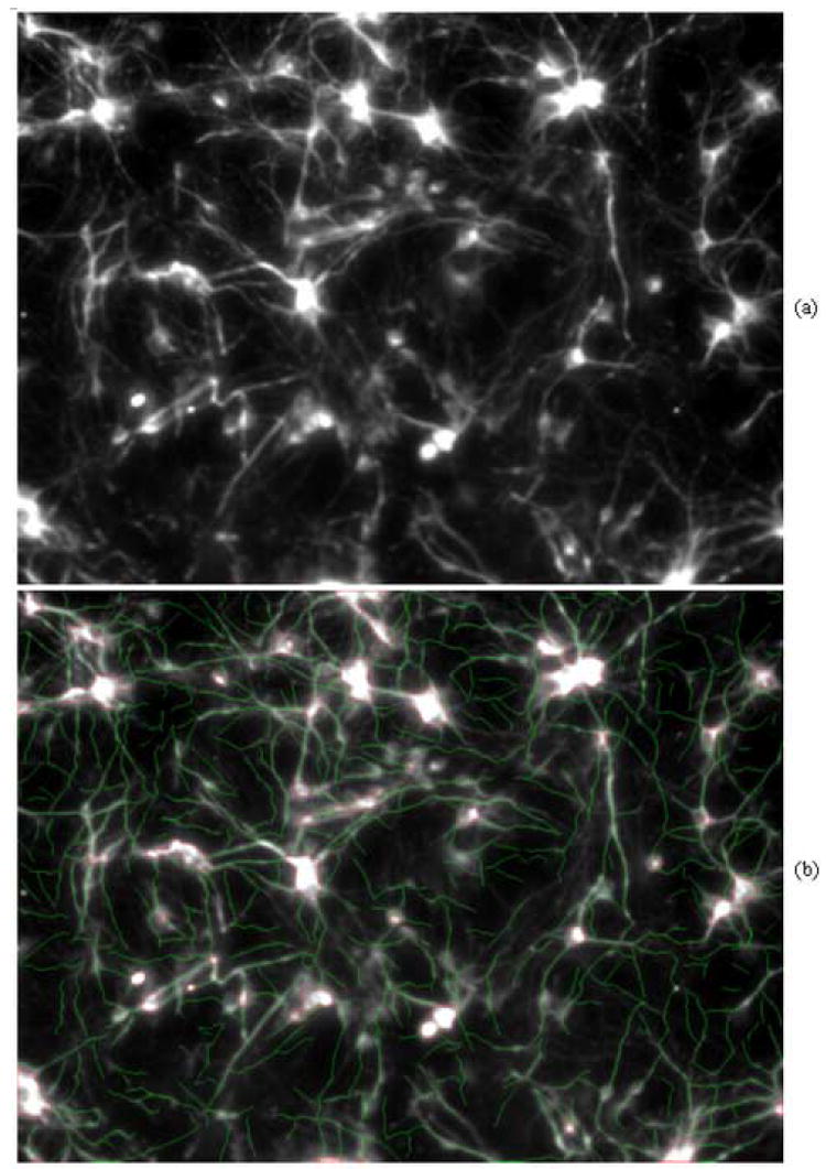
Sample result for neurite extraction. (a) original image; (b) result image with neurite segments labeled by green color and soma regions labeled by red color.

Fig. 6.

Sample result for neurite extraction. (a) original image; (b) result image with neurite segments labeled by green color and soma regions labeled by red color.

We also compare the extraction performance between our proposed method and the NeuronJ, a method proposed by Meijering et al (Meijering et al., 2004)and a plug-in tool of the ImageJ (Lydon, 2005).Figure 7 shows a partial image of neurite segments and two extraction results.Figure 7 (b) is the extraction result by NeuronJ. Note that the starting point and the ending point have to be specified by the user.Figure 7 (c) is the extraction result by our proposed method. The starting point and the ending points are automatically determined by the algorithm. It is clear to see that our proposed method has the extraction performance as accurate as that of NeuronJ and outperforms NeuronJ in terms of automation.

Fig. 7.

A partial image of neurite segment and two extraction results. (a) Original partial image; (b) Extraction result using NeuronJ; (c) Extraction result using our proposed method.

5.3 Validation

It is a difficult problem to evaluate the algorithm for automated neurite tracing, because manual labeling always has bias and different people may have quite different results. If the manual tracing is performed in a completely independent way and blinded to the algorithm, then the quantitative difference between the manual results and the automated results will be always quite huge. For example, users may randomly pick up a starting point and draw a centerline from that point and stop at any location they want. In images with complicated branching structures, human users may select a branch that is different from the one selected by the algorithm, even though the overall labels for the two methods could be very similar if examined visually.

If the manual tracing is guided by the automated results, then it is guaranteed that both human users and the algorithm use the same starting and ending points and select the same routine when tracing the complicated branching structures. Based on that, the human users still judge independently where the centerlines are located. We believe that using this method, the algorithm can be evaluated effectively and efficiently from both visual inspection and quantitative comparison.

The following experiment is used to quantitatively evaluate the neurite extraction performance of our proposed algorithm. We apply our algorithm on 100 neuron images to extract neurite segments. Then a total of 20 soma regions and their neurite segments are randomly selected from those images. Two independent individuals manually labelled the neurite segments in the twenty soma regions. The manual labeling process is guided by the computer generated results so that the two results can be compared for validation. Length difference and centerline deviation are the quantities used for evaluating the difference between the manual results and the computer generated results. The length difference (ϕ) is defined as follows: $\varphi =\mid 1-\frac{L_m}{L_c}\mid$, where L_m is the length of the neurite segment extracted manually, L_c is the length of the neurite segment generated by the algorithm. The centerline deviation (φ) is calculated as follows: $\phi =\frac{\mathit{Area}(l_c,l_m)}{L_c}$, where l_c and l_m are the centerlines of the neurite segments extracted automatically and manually, respectively. Area(l_c,l_m) represents the area of the region in pixels surrounded by l_c and l_m. Given ϕ and φ, we use the following methods to validate our results:

1. compare the mean and standard deviation of ϕ and φ between the two observers;

2. calculate the p-values of ϕ and φ using the two-sided paired t-test;

3. calculate the Pearson linear correlation coefficients of ϕ and φ;

4. calculate the cumulative distribution of ϕ and φ using Kolmogorov-Smirnov goodness-of-fit hypothesis test (Nimchinsky et al., 2002) and compare the quantile-quantile plots of the two observers.

Table 1 lists the mean and standard deviation of ϕ and φ for the two observers, as well as the p-values between them. The results show that the manual extractions between the two observers are very similar. Table 2 shows the Pearson linear correlation coefficients of ϕ and φ among the algorithm and the two observers. The coefficients indicate that there exist strong correlations between the computer generated results and Observer 1’s results, the computer generated results and Observer 2’s results, Observer 1’s results and Observer 2’s results. Figure 8 shows the box plots of the mean and standard deviation of ϕ and φ for the two observers, indicating that the quantitative results from the two observers are similar.

Table 1.

The mean and standard deviations of length difference and centerline deviation, and p-values for the two observers

	ϕ			φ
	Mean	Std	p-value	Mean	Std	p-value
Observer 1	0.0192	0.0244	0.5905	1.5705	0.1355	0.7518
Observer 2	0.0163	0.0183		1.5798	0.1405

Table 2.

The Pearson linear correlation coefficients between the results generated from the algorithm, the observer 1, and the observer 2

	ϕ			φ
	Algorithm	Observer 1	Observer 2	Algorithm	Observer 1	Observer 2
Algorithm	-	0.9946	0.9976	-	-	-
Observer 1	0.9946	-	0.9980	-	-	0.9053
Observer 2	0.9976	0.9980	-	-	0.9053	N/A

Fig. 8.

Box plots for the length difference and the centerline deviation. The red line is the mean value for each data set. The upper line of the box is the upper quartile value. The lower line of the box is the lower quartile value. (a) length difference of the two observers; and (b) center-line deviation of the two observers.

Figure 9 (a)-(c) displays the quantile-quantile plots of the length and the centerline deviation of the neurite segment observed by the two individuals. In the plots, the symbol “+” represents the length values or the deviation values. A green line joints the first and third quartiles of each distribution, which indicates that the two sets of quantitative values have a linear fit of the order statistics. The red line is the extension of the green line to the ends of the data set to help evaluate the linearity of the data. Figure 9 (d)-(f) shows the cumulative distributions of the length and the center-line deviation of the neurite segment observed by the two individuals. All the plots prove that the quantitative results obtained from the algorithm, and the two observers have the same or similar statistics distributions.

Fig. 9.

Quantile-quantile plots of the length of the neurite segment for (a) algorithm vs. Observer 1; (b) algorithm vs. Observer 2; quantile-quantile plots of the centerline deviation for (c) Observer 1 vs. Observer 2; cumulative distributions of the length of the neurite segment for (d) algorithm (green) vs. Observer 1 (red); (e) algorithm (green) vs. Observer 2 (red); cumulative distributions of the centerline deviation for (f) Observer 1 (green) vs. Observer 2 (red)

The test neuron images are also manually traced by two users in such a way that the manual labels are completely independent and blinded to the automated results. The Quantile-quantile plots and cumulative probability plots are displayed in Figure 10. From the figure we can see that the new line difference and centerline deviation are relatively larger than those if the manual results are guided by the automated results. However, the previous conclusions still hold. That is, the quantitative results from the two observers are still very similar. The quantitative results obtained from the algorithm, and the two observers have similar statistics distributions. The cumulative probability plots show that the independent manual results always have smaller line lengths compared to the automated results. This is due to the reason that the users always ignore some neurite centerlines, especially the weak lines.

Fig. 10.

Quantile-quantile plots of the length of the neurite segment for (a) algorithm vs. Observer 1; (b) algorithm vs. Observer 2; quantile-quantile plots of the centerline deviation for (c) Observer 1 vs. Observer 2; cumulative distributions of the length of the neurite segment for (d) algorithm (green) vs. Observer 1 (red); (e) algorithm (green) vs. Observer 2 (red); cumulative distributions of the centerline deviation for (f) Observer 1 (green) vs. Observer 2 (red)

5.4 Parameter selection

The parameters that may affect the extraction of neurite segments include maximum possible width W_max of the neurite segments, the standard deviation σ of the Gaussian kernel, and the weight ε for the cost function. We explain in the following how these parameters may affect the performance of the algorithm.

The maximum possible width W_max is used when detecting the ending point of a neurite segment. It defines the searching range when detecting the edge points by examining the maximum template responses. In high-throughput applications,W_max can be determined by looking into a single neuron image, and then it can be used for all the other neuron images acquired from the same experiment. In this paper, we use W_max=12 for all the 100 neuron images and the results are satisfactory.

The second-order derivative of the neuron image is estimated as the convolution of the image and the second-order derivative of a 2-D Gaussian kernel. The standard deviation σ of the kernel is then an important factor that determines whether or not the centerline of a neurite segment can be detected correctly. In (Steger, 1998), it was shown that the detectable line structures have a width between 0 and 2.5σ, if the second-order derivative of the image is used to detect the lines. In this paper, the second-order derivative of a neuron image is used in the cost function (see formula 21) to determine the probability of a pixel being on the neurite segment. Thus a lot of neurite segments with relatively large width will be ignored by using a small σ. If σ is selected large enough to cover most neurite segments, narrow segments with low intensity contrast will be smoothed out and parallel lines will affect each other. For example, in Figure 11 two extraction results are shown when using different σ. Obviously when σ = 6.5, the extracted center line is influenced by neighboring lines and the extraction is not satisfactory. In this paper, we use σ = 2.0 as a fixed value for all the neuron images from the same experiment. We believe that σ can be determined adaptively based on each neurite segment and its second-order derivatives. We will consider the automatic selection of σ in our future work.

Fig. 11.

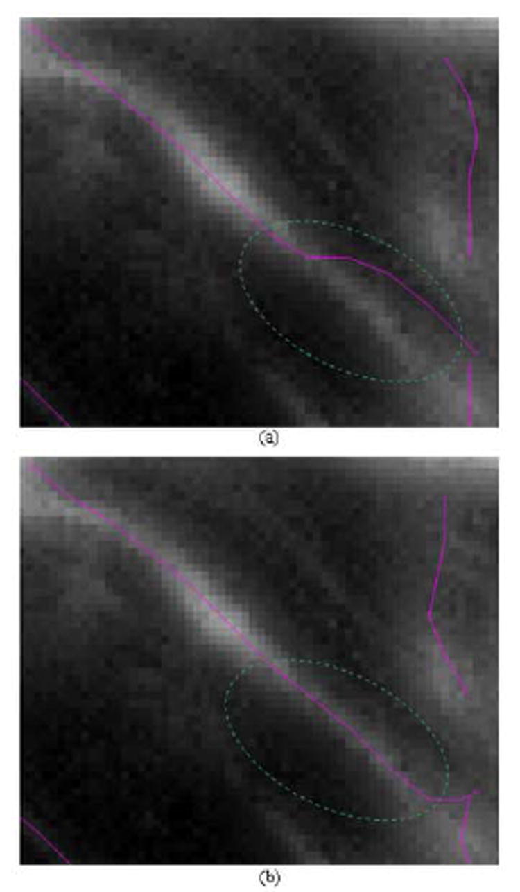
Comparison between extractions using different standard deviation values for the Gaussian kernel. A partial image is displayed with the extracted centerlines for the partial neurite segments are labeled in color. Note the difference of the lines within the two areas encircled by the dashed green circles. (a) partial image with extracted results for σ = 6.5 , and (b) partial image with extracted results for σ = 2.0.

The weight ε is used in the cost function defined in formula (21) to balance the influences of the two cost components. The local cost c_L(p) of a point p determines how well the extracted line approximates the centerline of the neurite segment. The linking cost c_D(p₁, p₂) of two points determines the best way to link the points on the centerline by examining the similarity between their gradient directions. Figure 12 compares two extractions when using weight 1 and 0 respectively. The results show that the centerline of a neurite segment may not be extracted accurately if the local cost is not considered. In Figure 13 we compare the extraction performance between the situation when only local cost is considered and the situation when both the local cost and the linking cost are considered. The results prove that, even though the centerline can be extracted in both cases, the linking between the centerline points is usually smoother and tighter to a strong edge if the linking cost is considered. In this paper, we use ε=0.8 for all the images.

Fig. 12.

Comparison between extractions using different weight values for the cost function. A partial image is displayed with the extracted centerlines for the partial neurite segments are labeled in color. Note the difference of the color lines in the middle of the image. (a) extraction results for ε = 1.0; (b) extraction results for ε = 0.0

Fig. 13.

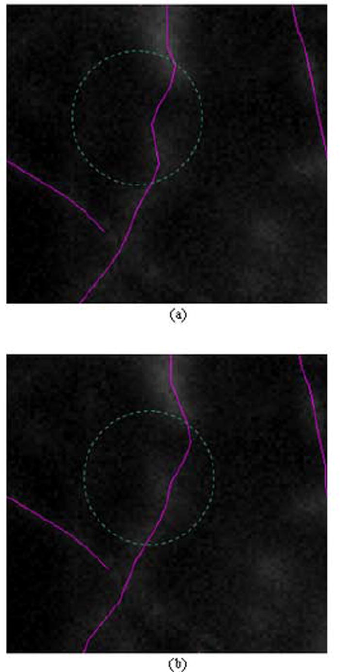
Comparison between extractions using different weight values for the cost function. A partial image is displayed with the extracted centerlines for the partial neurite segments are labeled in color. Note the difference of the lines within the two areas encircled by the dashed green circles. (a) extraction results forε = 1.0; (b) extraction results forε = 0.8

6. Conclusion

In this paper we present a novel algorithm for extraction of neurite structures in fluorescence microscopy neuron images. This algorithm is specifically designed for high-throughput screening of neuron-based assays, which usually requires the process to be fast and automatic. The algorithm is able to automatically select a pair of starting point and ending point for each neurite segment so that only minimum user interaction is required. The starting point is selected by detecting the local maxima after low-pass filtering a grid of lines in the image, followed by signal-to-noise ratio analysis to filter robust points. The automatic selection of the ending point is achieved by iteratively tracing the points on or near the centerline of the neurite segment until the end of the neurite structure. Robust starting points and redundant ending points are used so that the extraction is complete. Dynamic programming is used to link the points so that the centerline can be extracted rapidly, accurately, and smoothly. The results and validation indicate that our proposed algorithm can automatically and accurately extract most of the neurite segments in the image with complicated neurite structures. The algorithm is very efficient in applying the dynamic searching only on a small area of the image. All these advantages make the proposed algorithm suitable for the increasingly demanding and complex image analysis tasks in high-throughput neurite imaging applications and drug screening.

References

- Al-Kofahi KA, Can A, Lasek S, Szarowski DH, Dowell-Mesfin N, Shain W, Turner JN, Roysam B. Median-based robust algorithms for tracing neurons from noisy confocal microscope images. IEEE Transactions on Information Technology In Biomedicine. 2003;7:302–317. doi: 10.1109/titb.2003.816564. [DOI] [PubMed] [Google Scholar]
- Al-Kofahi KA, Lasek S, Szarowski DH, Pace CJ, Nagy G, Turner JN, Roysam B. Rapid automated three-dimensional tracing of neurons from confocal image stacks. IEEE Transactions on Information Technology in Biomedicine. 2002;6:171–187. doi: 10.1109/titb.2002.1006304. [DOI] [PubMed] [Google Scholar]
- Amini AA, Weymouth TE, Jain RC. Using dynamic programming for solving variational problems in vision. IEEE Transactions Pattern Analysis and Machine Intelligence. 1990;12:855–867. [Google Scholar]
- Barrett WA, Mortensen EN. Interactive live-wire boundary extraction. Medical Image Analysis. 1996;1:331–341. doi: 10.1016/s1361-8415(97)85005-0. [DOI] [PubMed] [Google Scholar]
- Bellman RE, Dreyfus SE. Applied dynamic programming. Princeton University Press; 1962. [Google Scholar]
- Cacace A, Banks M, Spicerb T, Civolic F, Watson J. An ultra-HTS process for the identification of small molecule modulators of orphan G-protein-coupled receptors. Drug Discovery Today. 2003;8:785–792. doi: 10.1016/s1359-6446(03)02809-5. [DOI] [PubMed] [Google Scholar]
- Can A, Shen H, Turner JN, Tanenbaum HL, Roysam B. Rapid automated tracing and feature extraction from live high-resolution retinal fundus images using direct exploratory algorithms. IEEE Transactions on Information Technology in Biomedicine. 1999;3:125–138. doi: 10.1109/4233.767088. [DOI] [PubMed] [Google Scholar]
- Chaudhuri S, Chatterjee S, Katz N, Nelson M, Goldbaum M. Detection of blood vessels in retinal images using two-dimensional matched filters. IEEE Transactions on Medical Imaging. 1989;3:263–269. doi: 10.1109/42.34715. [DOI] [PubMed] [Google Scholar]
- Coatrieux JL, Garreau M, Collorec R, Roux C. Computer vision approaches for the three-dimensional reconstruction: Review and prospects. Critical Reviews in Biomedical Engineering. 1994;22:1–38. [PubMed] [Google Scholar]
- Collorec R, Coatrieux JL. Vectorial tracking and directed contour finder for vascular network in digital subtraction angiography. Pattern Recognition Letters. 1988;8:353–358. [Google Scholar]
- Cormen TH, Leiserson CE, Rivest RL, Stein C. Introduction to algorithms. The MIT Press; 2001. [Google Scholar]
- Dijkstra EW. A note on two problems in connexion with graphs. Numerische Mathematik. 1959;1:269–271. [Google Scholar]
- Dunkle R. Role of Image informatics in accelerating drug discovery and development. Drug Discovery World. 2003;5:75–82. [Google Scholar]
- Falcão AX, Udupa JK, Miyazawa FK. An ultra-fast user-steered image segmentation paradigm: Livewire on the fly. IEEE Transactions on Medical Imaging. 2000;19:55–62. doi: 10.1109/42.832960. [DOI] [PubMed] [Google Scholar]
- Falcão AX, Udupa JK, Samarasekera S, Sharma S. User-steered image segmentation paradigms: Livewire and live lane. Graphical Models and Image Processing. 1998;60:233–260. [Google Scholar]
- Feng Y. Practicing cell morphology based screen. European Pharmaceutical Review. 2002;7:7–11. [Google Scholar]
- Florack LMJ, Romeny BMtH, Koenderink JJ, Viergever MA. Scale and the differential structure of images. Image and Vision Computing. 1992;10:376–388. [Google Scholar]
- Fox SJ. Accommodating cells in HTS. Drug Discovery World. 2003;5:21–30. [Google Scholar]
- Frangi AF, Niessen WJ, Hoogeveen RM, Walsum Tv, Viergever MA. Model-based quantitation of 3-D magnetic resonance angiographic images. IEEE Transactions on Medical Imaging. 1999;18:946–956. doi: 10.1109/42.811279. [DOI] [PubMed] [Google Scholar]
- Gaunitz F, Heise K. HTS compatible assay for antioxidative agents using primary cultured hepatocytes. ASSAY and Drug Development Technologies. 2003;1:469–477. doi: 10.1089/154065803322163786. [DOI] [PubMed] [Google Scholar]
- Geiger D, Gupta A, Costa LA, Vlontzos J. Dynamic programming for detecting, tracking, and matching deformable contours. IEEE Transactions on Pattern Analysis and Machine Intelligence. 1995;17:294–302. [Google Scholar]
- Iverson LA, Zucker SW. Logical/Linear operators for image curves. IEEE Transactions on Pattern Analys is and Machine Intelligence. 1995;17:982–996. [Google Scholar]
- Janssen RDT, Vossepoel AM. Adaptive vectorization of line drawing images. Computer vision and image understanding. 1997;65:38–56. [Google Scholar]
- Klyushnichenko V. Protein crystallization: from HTS to kilogram-scale. Current Opinion in Drug Discovery & Development. 2003;6:848–854. [PubMed] [Google Scholar]
- Kweon IS, Kanade T. Extracting topographic terrain features from elevation maps. Computer Vision, Graphics, and Image Processing: Image Understanding. 1994;59:171–182. [Google Scholar]
- Lindeberg T. Edge detection and ridge detection with automatic scale selection. International Journal of Computer Vision. 1998;30:117–154. [Google Scholar]
- Lydon JW. Geological Survey of Canada, Open File 4941. GEOSCAN; 2005. The measurement of the modal mineralogy of rocks from SEM imagery: the use of Multispec© and ImageJ freeware. [Google Scholar]
- Maintz JBA, Elsen PAvd, Viergever MA. Evaluation of ridge seeking operators for multimodality medical image matching. IEEE Transactions on Pattern Analysis and Machine Intelligence. 1996;18:353–365. [Google Scholar]
- Meijering E, Jacob M, Sarria J-CF, Steiner P, Hirling H, Unser M. Design and validation of a tool for neurite trac ing and analysis in fluorescence microscopy images. Cytometry. 2004;58A:167–176. doi: 10.1002/cyto.a.20022. [DOI] [PubMed] [Google Scholar]
- Mortensen E, Morse B, Barrett W, Udupa J. Computers in Cardiology 1992 Proceedings. Durham, NC: 1992. Adaptive boundary detection using ‘live-wire’ two-dimensional dynamic programming; pp. 635–638. [Google Scholar]
- Mortensen EN, Barrett WA. Interactive segmentation with intelligent scissors. Graphical Models and Image Processing. 1998;60:349–384. [Google Scholar]
- Nimchinsky EA, Sabatini BL, Svoboda K. Structure and function of dendritic spines. Annual review of physiology. 2002;64:313–353. doi: 10.1146/annurev.physiol.64.081501.160008. [DOI] [PubMed] [Google Scholar]
- Otsu N. A threshold selection method from gray-level histograms. IEEE Transactions on Systems, Man, and Cybernetics. 1979;9:62–66. [Google Scholar]
- Perlman ZE, Slack MD, Feng Y, Mitchison TJ, Wu LF, Altschuler SJ. Multid imens ional drug profiling by automated microscopy. Science. 2004;306:1194–1198. doi: 10.1126/science.1100709. [DOI] [PubMed] [Google Scholar]
- Polli R, Valli G. An algorithm for real-time vessel enhancement and detection. Comput Methods Programs Biomed. 1997;52:1–22. doi: 10.1016/s0169-2607(96)01773-7. [DOI] [PubMed] [Google Scholar]
- Sato Y, Nakajima S, Shiraga N, Atsumi H, Yoshida S, Koller T, Gerig G, Kikinis R. Three-dimensional multi-scale line filter for segmentation and visualization of curvilinear structures in medical images. Medical Image Analysis. 1998;2:143–168. doi: 10.1016/s1361-8415(98)80009-1. [DOI] [PubMed] [Google Scholar]
- Steger C. Extracting curvilinear structures: A differential geometric approach. In: Buxton BF, Cipolla R, editors. 4th European Conference on Computer Vision. Vol. 1064. Cambridge, UK: Springer; 1996. pp. 630–641. [Google Scholar]
- Steger C. An unbiased detector of curvilinear structure. IEEE Transactions on Pattern Analysis and Machine Intelligence. 1998;20:113–125. [Google Scholar]
- Sun Y, Lucariello RJ, Chiaramida SA. Directional lowpass filtering for improved accuracy and reproducibility of stenosis quantification in coronary arteriograms. IEEE Transactions on Medical Imaging. 1995;14:242–248. doi: 10.1109/42.387705. [DOI] [PubMed] [Google Scholar]
- Wang L, Pavlidis T. Detection of curved and straight segments from gray scale topography. Computer Vision, Graphics, and Image Processing: Image Understanding. 1993a;58:352–365. [Google Scholar]
- Wang L, Pavlidis T. Direct gray-scale extraction of features for character recognition. IEEE Transactions on Pattern Analysis and Machine Intelligence. 1993b;15:1053–1067. [Google Scholar]
- Wink O, Frangi AF, Verdonck B, Viergever MA, Niessen WJ. 3D MRA coronary axis determination using a minimum cost path approach. Magnetic Resonance in Medicine. 2002;47:1169–1175. doi: 10.1002/mrm.10164. [DOI] [PubMed] [Google Scholar]
- Yamada H, Merritt C, Kasvand T. Recognition of kidney glomerulus by dynamic programming matching method. IEEE Transactions Pattern Analysis and Machine Intelligence. 1988;10:731–737. [Google Scholar]
- Yarrow JC, Feng Y, Perlman ZE, Kirchhausen T, Mitchison TJ. Phenotypic screening of small molecule libraries by high throughput cell imaging. Combinatorial Chemistry & High Throughput Screening. 2003;6:279–286. doi: 10.2174/138620703106298527. [DOI] [PubMed] [Google Scholar]
- Zhang Y, Zhou X, Degterev A, Lipinski M, Adjeroh D, Yuan J, Wong STC. A novel tracing algorithm for high throughput imaging screening of neuron based assays. Journal of Neuroscience Methods. 2006 doi: 10.1016/j.jneumeth.2006.07.028. accepted for publication. [DOI] [PubMed] [Google Scholar]