Likelihood and Pseudo-likelihood Methods for Semiparametric Joint Models for a Primary Endpoint and Longitudinal Data

Abstract

Inference on the association between a primary endpoint and features of longitudinal profiles of a continuous response is of central interest in medical and public health research. Joint models that represent the association through shared dependence of the primary and longitudinal data on random effects are increasingly popular; however, existing inferential methods may be inefficient or sensitive to assumptions on the random effects distribution. We consider a semiparametric joint model that makes only mild assumptions on this distribution and develop likelihood-based inference on the association and distribution, which offers improved performance relative to existing methods that is insensitive to the true random effects distribution. Moreover, the estimated distribution can reveal interesting population features, as we demonstrate for a study of the association between longitudinal hormone levels and bone status in peri-menopausal women.

1 Introduction

Joint models that represent the association between a primary endpoint and features of longitudinal profiles of a related continuous response by shared dependence on underlying random effects have enjoyed increasing popularity when the focus of inference is on the strength and nature of the association. The primary endpoint may be a censored time-to-event (e.g. Henderson et al., 2000; Tsiatis and Davidian, 2004) or a single binary response, count, or other continuous measure. In the latter case, on which we focus, the joint model involves a linear mixed effects model (e.g. Laird and Ware, 1982), whose random effects characterize the salient features of the subject-specific longitudinal response profiles, linked to a generalized linear model (McCullagh and Nelder, 1989) for the primary endpoint, in which the random effects appear as covariates. Inference on the coefficients of these covariates addresses explicitly the association of interest.

A number of authors have proposed methods for implementation of this model. Wang et al. 2000 showed that replacing the random effects by subject-specific ordinary least squares estimators leads to biased estimation of primary model parameters. Wang et al. also proposed regression calibration (Carroll et al., 1995), which in this context involves replacing the random effects by estimated best linear unbiased predictors from a fit of the mixed effects model to the longitudinal profiles, assuming the random effects are normally distributed. Because this method does not entirely eliminate bias when the primary mean model is nonlinear, e.g. as for a binary endpoint, they also proposed a “refined” regression (RR) calibration technique for binary endpoint, which reduces or eliminates the bias but is still predicated on normality of the random effects. Concern over robustness of inference to departures from normality led Li et al. 2004 to a study of this issue, which showed that these methods can be alarmingly biased, inspiring these authors to extend methods of Stefanski and Carroll (1987) for generalized linear measurement error models to this setting. Li et al. 2004 derived so-called sufficiency score (SS) and conditional score (CS) methods, in which dependence on the random effects is removed by conditioning arguments, yielding estimators that are consistent regardless of the their distribution; see also Wang and Huang (2001). Li et al. demonstrated that SS and CS estimators are unbiased, yield valid inferences under departures from random effects normality, and are competitive to methods such as RR on basis of efficiency when normality does hold.

Because the SS and CS estimators “condition away” dependence on the random effects, they are valid under any true random effects distribution, including discrete or “unusual” distributions that are unlikely models for underlying features of profiles of continuous responses. Thus, although these methods enjoy robustness to nonnormality, the price is possible inefficiency relative to approaches that restrict to “plausible” distributional assumptions. Moreover, as the conditioning eliminates the random effects, these methods do not facilitate inference on the nature of the true random effects distribution, which may yield insight into inter-subject heterogeneity.

In this paper, we consider a semiparametric joint model in which the random effects distribution is left unspecified, as for SS and CS methods, but is assumed to lie in a broad class whose members have “smooth” densities that render them likely candidates to represent variation in subject-specific random effects for continuous longitudinal responses. The approach assumes that the linear mixed effects model for the longitudinal response is that of Zhang and Davidian (2001), in which the random effects density is assumed to lie in a class whose elements may be represented by the so-called “seminonparametric” (SNP) density estimator proposed by Gallant and Nychka (1987). Similar to Song et al. 2002 for a time-to-event endpoint, we develop likelihood-based inference for the primary model parameters and the random effects density.

In Section 2, we introduce data from the Study of Women’s Health Across the Nation (SWAN, Sowers et al., 2003), in which interest focuses on the association between characteristics of longitudinal hormone level profiles and a measure of bone mineral density in peri-menopausal women. In Section 3, the semiparametric joint model is described. We derive a full-likelihood-based implementation via the expectation-maximization (EM) algorithm in Section 4. When the primary endpoint is nonnormal, the EM involves computationally-expensive numerical integration; accordingly, in Section 5, we develop a less burdensome pseudo-likelihood approach. We apply both methods to the SWAN data in Section 6, and demonstrate performance in Section 7 via extensive simulations across a range of conditions.

2 The Study of Women Across the Nation

Low bone mineral density (BMD) is considered to be a key risk factor for osteoporosis, which afflicts 20% of US women over the age of 50 (Sowers et al., 2003), and an understanding of the relationship between monthly patterns of reproductive hormone levels and bone mineral density is thought to hold promise for identifying women for whom intervention to preserve bone mass may be indicated. The Study of Women’s Health Across the Nation (SWAN), a multi-ethnic cohort study enrolling over 3300 women undergoing transition to menopause examining physical, biological, psychological and social changes, offers a rich resource for studying this issue. In a SWAN substudy, the Daily Hormone Study (Santoro et al., 2004), total hip BMD (g/cm²) was measured for each participant at a clinical visit, and longitudinal urine samples were collected over an adjacent menstrual cycle and assayed for levels of several reproductive hormones. In addition, a number of subject characteristics, including body mass index (BMI, kg/m²), age (years), and ethnicity (Black, White, Chinese, Japanese), were recorded for each woman.

We focus on progesterone (pregnanediol glucuronide, PDG, μg/mg creatinine), a hormone implicated in fertility, available for 624 women in the substudy. Because women experience different cycle lengths, it is conventional to standardize to a 28-day reference (e.g. Zhang et al., 1998); Figure 1 shows longitudinal log PDG plotted against standardized days for 4 women. As noted by Li et al. 2004, profiles are fairly constant up to 14 days, then exhibit an apparent approximately symmetric rise and fall for the remainder of the cycle. Letting W_ij denote log PDG for woman i on standardized day t_ij, Li et al. 2004 represented the profile for woman i as

Figure 1.

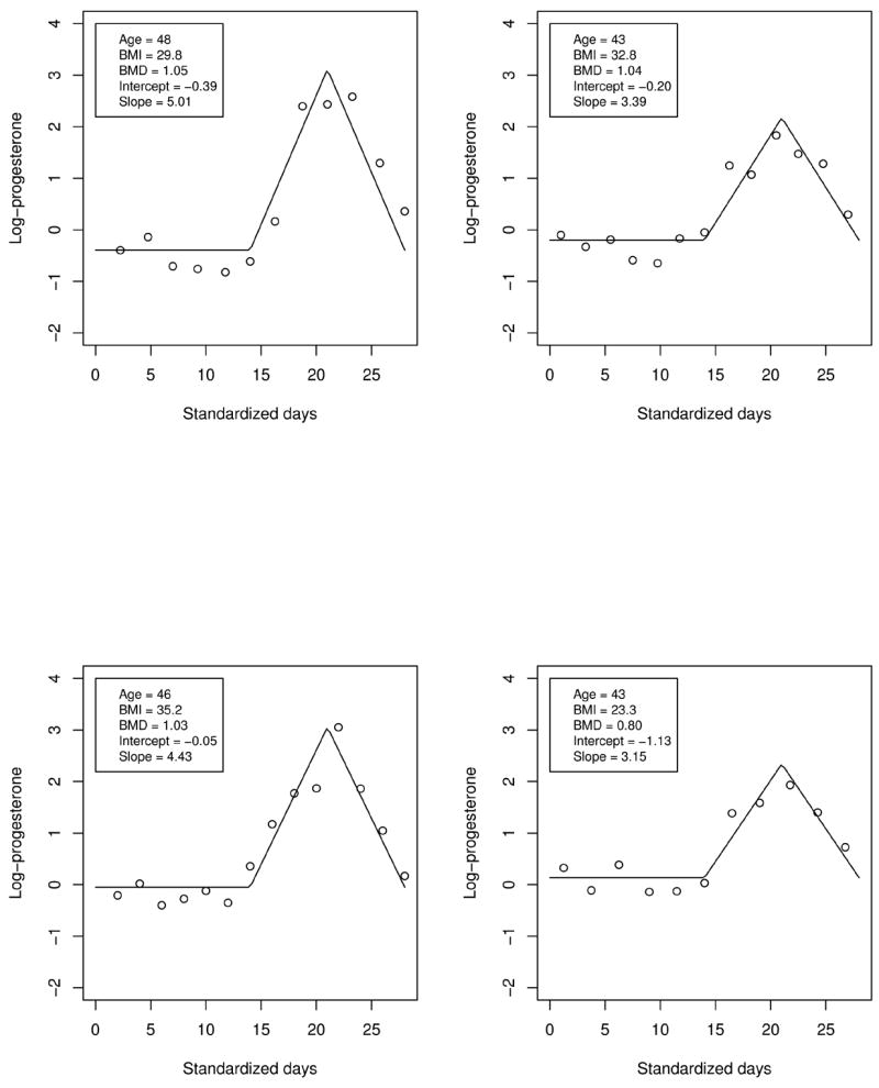
Natural logarithm of PDG levels (μg/mg creatinine) for four randomly selected women with individual ordinary least squares fits of the piecewise linear model (1) superimposed.

$$W_{ij}=X_{1i}+X_{2i}{(t_{ij}-14)}_{+}-2X_{2i}{(t_{ij}-21)}_{+}+U_{ij},$$ (1)

where i = 1, …, n(= 624), j = 1, …, m_i, u₊ = u if u > 0 and 0 otherwise, X_1i is the woman-specific constant log PDG up to day 14, X_2i is the “slope” of the symmetric rise (days 14–21) and fall (days 21–28) observed in Figure 1, and U_ij is a $\mathcal{N}(\text{0},{\sigma }_u^2)$ deviation representing within-woman variation and measurement error. The subset of the data we consider includes available every-other-day PDG measurements for each woman; m_i ranges from 8 to 25. In (1), X_1i and X_2i summarize for woman i the prominent features of the profiles: the first-cycle-half log PDG level and the second-cycle-half steepness of log PDG rise and fall, respectively.

Osteopenia, a precursor condition to osteoporosis, is characterized by low BMD (at or below the 33rd percentile). Letting Y_i = 1 denote absence of osteopenia for woman i, to characterize the association between presence/absence of osteopenia and the longitudinal pattern of log PDG, summarized by X_i = (X_1i, X_2i)^T, a natural framework is the logistic regression model

$$\text{pr}(Y_i=1\mid {\mathit{X}}_i;\mathit{\beta })={[1+exp\{-({\mathit{\beta }}_0^{\text{T}}{\mathit{C}}_i+{\mathit{\beta }}_1^{\text{T}}{\mathit{X}}_i)\}]}^{-1},\hspace{0.17em}\hspace{0.17em}\hspace{0.17em}\mathit{\beta }={({\mathit{\beta }}_0^{\text{T}},{\mathit{\beta }}_1^{\text{T}})}^{\text{T}},$$ (2)

where C_i is a vector of additional covariates (e.g. BMI, age, ethnicity) whose effects are to be taken into account. Model (2) represents the relationship between features of log PDG profiles and the primary endpoint osteopenia through shared dependence on X_i, and inference on β₀ and β₁ addresses formally this association and that between osteopenia and other subject attributes. As we discuss in the next section, (1) and (2) together define a joint model.

3 Semiparametric Joint Model

Generalizing the situation for SWAN in Section 2, suppose that for each subject i = 1, …, n, longitudinal measurements (W_1i, …, W_imi)^T at times t_1i, …, t_imi follow the linear mixed model

$${\mathit{W}}_i={\mathit{D}}_i{\mathit{X}}_i+{\mathit{U}}_i,$$ (3)

where D_i is a full-rank (m_i × q) design matrix; X_i is a (q × 1) random effect representing unobserved subject-specific features of the longitudinal profiles; and U_i = (U_i1, …, U_imi)^T are within-subject deviations, independent of X_i, independently and identically distributed as ${\mathit{U}}_i\sim \mathcal{N}(0,{\sigma }_u^2{\mathit{I}}_{m_i})$ for (l × l) identity matrix I_l. Let Y_i denote the primary endpoint and C_i (p × 1) be a vector of covariates for subject i. To relate the primary endpoint to features of the longitudinal profiles and covariates, assume the generalized linear model in canonical form given by the conditional density of Y_i given X_i and C_i (we suppress conditioning on C_i throughout)

$$f(Y_i\mid {\mathit{X}}_i;\mathit{\beta },\rho )=exp\left\{\frac{Y_i({\mathit{\beta }}_0^{\text{T}}{\mathit{C}}_i+{\mathit{\beta }}_1^{\text{T}}{\mathit{X}}_i)-b({\mathit{\beta }}_0^{\text{T}}{\mathit{C}}_i+{\mathit{\beta }}_1^{\text{T}}{\mathit{X}}_i)}{a(\rho )}+c(Y_i,\rho )\right\},$$ (4)

Where C_i has first element 1 when an intercept is included; $\mathit{\beta }={({\mathit{\beta }}_0^{\text{T}},{\mathit{\beta }}_1^{\text{T}})}^{\text{T}}$ are regression parameters; ρ is a dispersion parameter; and a(·), b(·), and c(·, ·) are known functions. Conditional on X_i, we take Y_i and W_i to be independent, the surrogacy assumption (e.g., Carroll et al., 1995).

The standard assumption for the distribution of the random effects is normality; however, this may characterize poorly heterogeneity in features of subject-specific profiles. Accordingly, supposing that random effects for a continuous response would themselves be continuous, Zhang and Davidian (2001) proposed replacing this assumption for the linear mixed model by the broader assumption that the random effects have density in a class of “smooth” differentiable densities studied by Gallant and Nychka (1987) that includes normal, multimodal, skewed, and heavy- or thin-tailed but not “unusual” densities. Densities in the class may be approximated by truncated series expansion referred to as “seminonparametric” (SNP), where the degree of truncation dictates the flexibility of the representation. Thus, following these authors, let

$${\mathit{X}}_i=\mathit{\mu }+\mathit{R}{\mathit{Z}}_i,$$ (5)

where μ is a q-dimensional vector of parameters, R is a (q × q) lower-triangular matrix, and the random vector Z_i (q × 1) has density that may be approximated by the SNP density

$$h_K(\mathit{z})=P_K^2(\mathit{z})\varphi (\mathit{z})={\left(\sum _{\mid \lambda \mid \le K}{a}_{\lambda }{\mathit{z}}^{\lambda }\right)}^2\varphi (\mathit{z}).$$ (6)

Here, P_K (z) is a Kth order polynomial with coefficients a_λ chosen so that (6) is a density, ϕ(·) is the $\mathcal{N}(0,{\mathit{I}}_q)$ density, λ = (λ₁, …, λ_q) is a vector of non-negative integers, and z^λ is the monomial ${\mathit{z}}^{\lambda }=z_1^{{\lambda }_1}\cdots z_q^{{\lambda }_q}$ of order $\mid \lambda \mid \hspace{0.17em}=\hspace{0.17em}{\sum }_{l=1}^q{\lambda }_l$. E.g., in the case q = 2 of interest in SWAN, z = (z₁, z₂)^T, P_K (z) = a₀₀ + a₁₀z₁ + a₀₁z₂ when K = 1 and $P_K(\mathit{z})=a_{00}+a_{10}{z}_1+a_{01}{z}_2+a_{20}{z}_1^2+a_{11}{z}_1{z}_2+a_{02}{z}_2^2$ when K = 2. Zhang and Davidian (2001) showed that ∫ h_K (z)dz = 1 holds if the collection a of the a_λ satisfies a^TAa = c^Tc = 1 for a certain known positive definite matrix A depending on q and K, which may be imposed by a radial transformation. E.g. with q = 2, a is of dimension d = (K + 1)(K + 2)/2, and take c₁ = sin(φ₁), c₂ = cos(φ₁) sin(φ₂), …, c_d−1 = cos(φ₁) cos(φ₂) … cos(φ_d−2) sin(φ_d−1), c_d = cos(φ₁) cos(φ₂) … cos(φ_d−1), where −π/2 < φ_l ≤ π/2 for l = 1, …, d − 1; when K = 2, a = (a₀₀, a₁₀, a₀₁, a₂₀, a₁₁, a₀₂)^T and d = 6. Parameterization of (6) in terms of φ = (φ₁, …, φ_d−1)^T thus ensures it is a density, and it follows that when K = 0, (6) reduces to the $\mathcal{N}(0,\mathit{R}{\mathit{R}}^{\text{T}})$ density. The choice of K is discussed in Section 4.

Letting r = vech(R), the non-zero elements of R, for given K, $\mathit{\theta }={({\mathit{\beta }}^{\text{T}},\rho ,{\sigma }_u^2,{\mathit{\mu }}^{\text{T}},{\mathit{r}}^{\text{T}},{\mathit{\phi }}^{\text{T}})}^{\text{T}}$ characterizes the proposed joint model. Inference on θ thus addresses not only the association, through β, but also yields an explicit estimate of the density through (μ, r, φ).

4 Full-likelihood Inference

With Y = (Y₁, …, Y_n)^T, $\mathit{W}={({\mathit{W}}_1^{\text{T}},\dots ,{\mathit{W}}_n^{\text{T}})}^{\text{T}}$, the observed-data loglikelihood for θ is

$$\ell (\mathit{\theta };\mathit{Y},\mathit{W})=\sum _{i=1}^{n}logf(Y_i,{\mathit{W}}_i;\mathit{\theta })=\sum _{i=1}^{n}log\left\{\int f(Y_i,{\mathit{W}}_i\mid \mathit{z};\mathit{\theta })P_K^2(\mathit{z};\mathit{\theta })\varphi (\mathit{z})d\mathit{z}\right\}$$ (7)

for fixed K, where we now emphasize dependence of P_K on θ, f (Y_i, W_i; θ) is the density of (Y_i, W_i), and f (Y_i, W_i|Z_i; θ) is the conditional density of (Y_i, W_i) given Z_i.

When Y_i is normally distributed given X_i (and C_i), (4) implies $Y_i={\mathit{\beta }}_0^{\text{T}}{\mathit{C}}_i+{\mathit{\beta }}_1^{\text{T}}{\mathit{X}}_i+{\epsilon }_i,\hspace{0.17em}{\epsilon }_i\sim \mathcal{N}(0,\rho )$. Here, f (Y_i; W_i|Z_i; θ)ϕ(Z_i) can be viewed as the joint density of (Y_i; W_i; Z_i) when Z_i is assumed to be $\mathcal{N}(0,{\mathit{I}}_q)\hspace{0.17em}[\text{so\hspace{0.17em}}{\mathit{X}}_i\sim \mathcal{N}(\mathit{\mu },\mathit{R}{\mathit{R}}^{\text{T}})]$. Letting g(Y_i, W_i; θ) denote the density of (Y_i, W_i) and g(Z_i|Y_i, W_i; θ) denote the conditional density of Z_i given (Y_i, W_i) when Z_i is standard normal, f (Y_i, W_i|Z_i; θ)ϕ(Z_i) = g(Y_i, W_i; θ)g(Z_i|Y_i, W_i; θ) and hence

$$f(Y_i,{\mathit{W}}_i;\mathit{\theta })=g(Y_i,{\mathit{W}}_i;\mathit{\theta })\int P_K^2(\mathit{z};\mathit{\theta })g(\mathit{z}\mid Y_i,{\mathit{W}}_i;\mathit{\theta })d\mathit{z}=g(Y_i,{\mathit{W}}_i;\mathit{\theta }){\text{E}}_{Z_i\mid Y_i,W_i;\theta }\{P_K^2({\mathit{Z}}_i;\mathit{\theta })\},$$

where E_Zi|YiWiθ (·) represents expectation with respect to the conditional distribution of (normal) Z_i given (Y_i, W_i). It is straightforward to show that g(Y_i, W_i; θ) is the normal density with mean ${\mathit{\eta }}_i={\{{\mathit{\beta }}_0^{\text{T}}{\mathit{C}}_i+{\mathit{\beta }}_1^{\text{T}}\mathit{\mu },{({\mathit{D}}_i\mathit{\mu })}^{\text{T}}\}}^{\text{T}}$ and covariance matrix

$${\mathbf{\Omega }}_i=\left(\begin{array}{ll}{\mathit{\beta }}_1^{\text{T}}\mathit{R}{\mathit{R}}^{\text{T}}{\mathit{\beta }}_1+\rho ,\hfill & {\mathit{\beta }}_1^{\text{T}}\mathit{R}{\mathit{R}}^{\text{T}}{\mathit{D}}_i^{\text{T}}\hfill \\ {\mathit{D}}_i\mathit{R}{\mathit{R}}^{\text{T}}{\mathit{\beta }}_1,\hfill & {\mathit{D}}_i\mathit{R}{\mathit{R}}^{\text{T}}{\mathit{D}}_i^{\text{T}}+{\sigma }_u^2{\mathit{I}}_{m_i}\hfill \end{array}\right),$$

and that g(Z_i|Y_i, W_i; θ) is the normal density with mean and covariance matrix

$${\mathit{\eta }}_i^{\ast }={\left(\begin{array}{l}{\mathit{\beta }}_1^{\text{T}}\mathit{R}\hfill \\ {\mathit{D}}_i\mathit{R}\hfill \end{array}\right)}^{\text{T}}{\mathbf{\Omega }}_i^{-1}\left\{\left(\begin{array}{c}{Y}_i\\ {\mathit{W}}_i\end{array}\right)-{\mathit{\eta }}_i\right\},\hspace{0.17em}\hspace{0.17em}\hspace{0.17em}{\mathbf{\Omega }}_i^{\ast }={\mathit{I}}_q-{\left(\begin{array}{l}{\mathit{\beta }}_1\mathit{R}\hfill \\ {\mathit{D}}_i\mathit{R}\hfill \end{array}\right)}^{\text{T}}{\mathbf{\Omega }}_i^{-1}\left(\begin{array}{l}{\mathit{\beta }}_1^{\text{T}}\mathit{R}\hfill \\ {\mathit{D}}_i\mathit{R}\hfill \end{array}\right).$$

Hence the observed-data loglikelihood (7) becomes

$$\ell (\mathit{\theta };\mathit{Y},\mathit{W})=\sum _{i=1}^{n}log\hspace{0.17em}\{g(Y_i,{\mathit{W}}_i;\mathit{\theta })\}+\sum _{i=1}^{n}log\hspace{0.17em}\left[E_{Z_i\mid Y_i,W_i;\theta }\{P_K^2({\mathit{Z}}_i;\mathit{\theta })\}\right],$$ (8)

where the first term is the usual loglikelihood for the normal model for (Y_i, W_i) with mean η_i and covariance matrix Ω_i, i = 1, …, n, which has a closed form; and the second term involves moments of a $\mathcal{N}({\mathit{\eta }}_i^{\ast },{\mathbf{\Omega }}_i^{\ast })$ random vector and also has a closed form that may be calculated using the series representation of the moment generating function of a normal random variable similar to Zhang and Davidian (2001). Thus, for normal Y_i, (8) has a closed-form expression and so may be maximized in θ using standard optimization software.

When Y_i is not normal, (7) does not have a closed-form representation. In principle, (7) may be maximized in θ by carrying out the required numerical integrations, but this can lead to computational instability. Accordingly, we derive an EM algorithm. Treating the random effects $\mathit{X}={({\mathit{X}}_1^{\text{T}},\dots ,{\mathit{X}}_n^{\text{T}})}^{\text{T}}$ as missing data, the complete-data (Y, W, X) likelihood for θ is

$$L_c(\mathit{\theta };\mathit{Y},\mathit{W},\mathit{X})=\prod _{i=1}^n\{f(Y_i\mid {\mathit{X}}_i;\mathit{\beta },\rho )f({\mathit{W}}_i\mid {\mathit{X}}_i;{\sigma }_u^2)f({\mathit{X}}_i;\mathit{\mu },\mathit{r},\mathit{\phi })\}$$ (9)

for fixed K, where f (Y_i|X_i; β, ρ) is as in (4), $f({\mathit{W}}_i\mid {\mathit{X}}_i;{\sigma }_u^2)$ is the $\mathcal{N}({\mathit{D}}_i{\mathit{X}}_i,{\sigma }_u^2{\mathit{I}}_{m_i})$ density as in (3), and $f({\mathit{X}}_i;\mathit{\mu },\mathit{r},\mathit{\phi })=P_K^2\{{\mathit{R}}^{-1}({\mathit{X}}_i-\mathit{\mu });\mathit{\theta }\}\varphi \{{\mathit{R}}^{-1}({\mathit{X}}_i-\mathit{\mu })\}\mid \mathit{R}{\mid }^{-1}$ is the representation of the density of X_i. The maximum likelihood estimator θ̂ is obtained by iterating between an E-step and an M-step to convergence. Let θ̂^(l) denote the estimate at the lth iteration. In the E-step, compute Q(θ|θ̂^(l)) = E{log L_c(θ; Y, W, X)|Y, W ; θ̂^(l)}, i.e. the conditional expectation of the logarithm of (9) given the observed data and current parameter estimates. In the M-step, maximize Q(θ|θ̂^(l)) with respect to θ to obtain the update θ̂^(l+1).

At the (l + 1)th iteration, it may be shown that

$${\widehat{{\sigma }_u^2}}^{(l+1)}=\sum _{i=1}^{n}E\{{({\mathit{W}}_i-{\mathit{D}}_i{\mathit{X}}_i)}^{\text{T}}({\mathit{W}}_i-{\mathit{D}}_i{\mathit{X}}_i)\mid Y_i,{\mathit{W}}_i;{\widehat{\mathit{\theta }}}^{(l)}\}/\sum _{i=1}^n{m}_i.$$

The updates ( ${\widehat{\mathit{\beta }}}_0^{(l+1)},{\widehat{\mathit{\beta }}}_1^{(l+1)},{\widehat{\rho }}^{(l+1)}$) maximize

$$\sum _{i=1}^n\left([Y_i{\mathit{\beta }}_0^{\text{T}}{\mathit{C}}_i+Y_i{\mathit{\beta }}_1^{\text{T}}E({\mathit{X}}_i\mid Y_i,{\mathit{W}}_i;{\widehat{\mathit{\theta }}}^{(l)})-E\{b({\mathit{\beta }}_0^{\text{T}}{\mathit{C}}_i+{\mathit{\beta }}_1^{\text{T}}{\mathit{X}}_i)\mid Y_i,{\mathit{W}}_i;{\widehat{\mathit{\theta }}}^{(l)}\}]/a(\rho )+c(Y_i,\rho )\right).$$

They may also be obtained by a one-step Newton-Raphson approximation similar to Wulfsohn and Tsiatis (1997). Letting γ = (β^T, ρ)^T, the updates are, ${\widehat{\mathit{\gamma }}}^{(l+1)}={\widehat{\mathit{\gamma }}}^{(l)}+I_{{\widehat{\gamma }}^{(l)}}^{-1}{S}_{{\widehat{\gamma }}^{(l)}}$, where S_γ̂^l) and I_γ̂^(l) are the score vector and information matrix for γ at the lth iteration, respectively; e.g. for the logistic primary endpoint model as in (2), γ = β and

$$S_{{\widehat{\beta }}^{(l)}}=\left(\begin{array}{l}{\sum }_{i=1}^n\{Y_i-E(v_i\mid Y_i,{\mathit{W}}_i;{\widehat{\mathit{\theta }}}^{(l)})\}{\mathit{C}}_i\hfill \\ {\sum }_{i=1}^n\{Y_{i}E({\mathit{X}}_i\mid Y_i,{\mathit{W}}_i;{\widehat{\mathit{\theta }}}^{(l)})-E(v_i{\mathit{X}}_i\mid Y_i,{\mathit{W}}_i;{\widehat{\mathit{\theta }}}^{(l)})\}\hfill \end{array}\right),$$

$$I_{{\widehat{\beta }}^{(l)}}=\left(\begin{array}{ll}{\sum }_{i=1}^{n}E\{(v_i-v_i^2)\mid Y_i,{\mathit{W}}_i;{\widehat{\mathit{\theta }}}^{(l)}\}{\mathit{C}}_i{\mathit{C}}_i^{\text{T}},\hfill & {\sum }_{i=1}^n{\mathit{C}}_i^{\text{T}}E\{(v_i-v_i^2){\mathit{X}}_i^{\text{T}}\mid Y_i,{\mathit{W}}_i;{\widehat{\theta }}^{(l)}\}\hfill \\ {\sum }_{i=1}^{n}E\{(v_i-v_i^2){\mathit{X}}_i\mid Y_i,{\mathit{W}}_i;{\widehat{\mathit{\theta }}}^{(l)}\}{\mathit{C}}_i\hfill & {\sum }_{i=1}^{n}E\{(v_i-v_i^2){\mathit{X}}_i{\mathit{X}}_i^{\text{T}}\mid Y_i,{\mathit{W}}_i;{\widehat{\theta }}^{(l)}\}\hfill \end{array}\right),$$

where $v_i={[1+exp\{-({\widehat{\mathit{\beta }}}_0^{(l)\text{T}}{\mathit{C}}_i+{\widehat{\mathit{\beta }}}_1^{(l)\text{T}}{\mathit{X}}_i)\}]}^{-1}$. As P_K depends on θ only through φ, in (9), the parameters (μ, r, φ) in the SNP density representation are separated from the others, so that iterative updates (μ^(l+1), r^(l+1), φ^(l+1)) are obtained by maximizing

$$\sum _{i=1}^n\left(E[log{P}_K^2\{{\mathit{R}}^{-1}({\mathit{X}}_i-\mathit{\mu });\mathit{\theta }\}\mid Y_i,{\mathit{W}}_i;{\widehat{\mathit{\theta }}}^{(l)}]+E[log\varphi \{{\mathit{R}}^{-1}({\mathit{X}}_i-\mathit{\mu })\}\mid Y_i,{\mathit{W}}_i;{\widehat{\mathit{\theta }}}^{(l)}]-log\mid \mathit{R}\mid \right),$$

which may be carried out using a standard optimizer.

These expressions all involve integrals of the form E{s(X _i)|Y_i, W_i; θ̂^(l)} = ∫ s(x)f(x|Y_i, W_i; θ̂^(l))dx, where s(X_i) is a function of X_i and f (X_i|Y_i, W_i; θ) is the conditional density of X_i given the observed data (Y_i, W_i). These integrals must be computed numerically, facilitated by noting

$$f({\mathit{X}}_i\mid Y_i,{\mathit{W}}_i;{\widehat{\mathit{\theta }}}^{(l)})=\frac{f(Y_i,{\mathit{W}}_i,{\mathit{X}}_i;{\widehat{\mathit{\theta }}}^{(l)})}{\int f(Y_i,{\mathit{W}}_i,\mathit{x};{\widehat{\mathit{\theta }}}^{(l)})d\mathit{x}},$$

where $f(Y_i,{\mathit{W}}_i,{\mathit{X}}_i;{\widehat{\mathit{\theta }}}^{(l)})=f(Y_i\mid {\mathit{X}}_i;{\widehat{\mathit{\beta }}}^{(l)},{\widehat{\rho }}^{(l)})f({\mathit{W}}_i\mid {\mathit{X}}_i;{\widehat{{\sigma }_u^2}}^{(l)})f({\mathit{X}}_i;{\widehat{\mathit{\mu }}}^{(l)},{\widehat{\mathit{r}}}^{(l)},{\widehat{\mathit{\phi }}}^{(l)})$, which has an explicit expression. Our implementation uses Gauss-Hermite quadrature.

To obtain the starting value θ̂⁽⁰⁾ for given K, we use the estimates of $(\mathit{\beta },\rho ,{\sigma }_u^2)$ from the conditional score method of Li et al. 2004, which is fast and straightforward to implement and yields consistent estimators regardless of the true random effects distribution. For the starting values for the parameters in the SNP density representation, we fit (3) via the approach of Zhang and Davidian (2001) for the chosen K, and use the resulting estimates of (μ, r, φ).

Standard errors for the final estimator θ̂ for given K may be derived from the inverse of the observed information, i.e. the second derivative matrix of (7) evaluated at θ̂, which may be carried out using numerical integration (e.g. Gauss-Hermite quadrature) or Monte Carlo approximation as in Chen et al. 2002; we use the former in the analyses of subsequent sections.

The preceding development is for fixed K. In practice, the analyst may take K > 0 fixed to allow for departures from normality. Alternatively, it is standard to choose K via objective information criteria, fitting the model for different K and selecting the K that minimizes a penalized version of the maximized observed-data loglikelihood; i.e. −ℓ(θ̂; Y, W)/N + C(N)(p/N), where $N=n+{\sum }_{i=1}^n{m}_i$ is the total number of observations; p = dim(θ); and C(N ) is a penalty factor equal to 1 for Akaike’s Information Criterion (AIC), log(log N) for the Hannan-Quinn Criterion (HQ), and (log N)/2 for the Schwarz Information Criterion (BIC). Practically, the analyst may increase K from 0 until K_max when an information criterion no longer decreases; often K_max up to 2 suffices in practice for representing complicated shapes, as demonstrated in Sections 6 and 7. Zhang and Davidian (2001) discussed the relative merits of these criteria, noting that HQ tends to offer a compromise between AIC and BIC.

Based on the final chosen K, inference on individuals is possible via the empirical Bayes approach of Davidian and Gallant (1993), where “estimates” X̂_i of subject-specific random effects X_i are obtained as posterior modes; i.e. X̂_i = arg max_Xi f(X_i|Y_i, W_i; θ̂).

5 Pseudo-likelihood Inference

For nonnormal Y_i, the EM algorithm in Section 4 can be computationally burdensome. We thus consider an alternative approach to inference on θ under the semiparametric joint model that exploits the fact that $(\mathit{\mu },\mathit{r},\mathit{\phi },{\sigma }_u^2)$ may be estimated based on W and the mixed model (3) only. We propose a two-step scheme: (i) estimate $(\mathit{\mu },\mathit{r},\mathit{\phi },{\sigma }_u^2)$ by fitting the mixed model (3) to the data W via the approach of Zhang and Davidian (2001), selecting K by inspection of a suitable information criterion; and (ii) estimate the remaining parameters (β, ρ) characterizing (4) via an approach similar to that of Carroll et al. 1984, maximizing $p\ell (\mathit{\theta };\mathit{Y},\mathit{W})={\sum }_{i=1}^{n}logf(Y_i\mid {\mathit{W}}_i;\mathit{\theta })$ in (β, ρ) holding $(\mathit{\mu },\mathit{r},\mathit{\phi },{\sigma }_u^2)$ fixed at the estimates from (i), where f (Y_i|W_i; θ) is the conditional density of Y_i given W_i. We may regard (ii) as a “pseudo-likelihood" approach, where the “nuisance parameters” $(\mathit{\mu },\mathit{r},\mathit{\phi },{\sigma }_u^2)$ are held fixed at previous estimates.

We thus derive the form of f(Y_i|W_i; θ). It is easy to see that

$$f(Y_i\mid {\mathit{W}}_i;\mathit{\theta })=\frac{\int f(Y_i\mid \mathit{z};\mathit{\theta })f({\mathit{W}}_i\mid \mathit{z};\mathit{\theta })P_K^2(\mathit{z};\mathit{\theta })\varphi (\mathit{z})d\mathit{z}}{f({\mathit{W}}_i;\mathit{\theta })},$$

where f(Y_i|Z_i; θ) and f (W_i|Z_i; θ) are the density of (4) and the normal density of W_i given X_i, respectively, with X_i replaced by μ + RZ_i; and f(W_i; θ) is the marginal density of the longitudinal data. Note that f(W_i|Z_i; θ)ϕ(Z_i) can be viewed as the joint density of W_i and Z_i when ${\mathit{Z}}_i\sim \mathcal{N}(0,{\mathit{I}}_q)$. Let f* (Z_i|W_i; θ) and f* (W_i; θ) denote the conditional density of Z_i given W_i and the marginal density of W_i when ${\mathit{Z}}_i\sim \mathcal{N}(0,{\mathit{I}}_q)$, respectively. Then f (W_i|Z_i; θ)ϕ(Z_i) = f* (Z_i|W_i; θ) f* (W_i; θ) and in fact

$$\begin{array}{l}f({\mathit{W}}_i;\mathit{\theta })=\int f({\mathit{W}}_i\mid \mathit{z};\mathit{\theta })P_K^2(\mathit{z};\mathit{\theta })\varphi (\mathit{z})d\mathit{z}=f^{\ast }({\mathit{W}}_i;\mathit{\theta })\int P_K^2(\mathit{z};\mathit{\theta })f^{\ast }(\mathit{z}\mid {\mathit{W}}_i;\mathit{\theta })d\mathit{z}\\ =f^{\ast }({\mathit{W}}_i;\mathit{\theta })E_{Z_i\mid W_i}\{P_K^2({\mathit{Z}}_i;\mathit{\theta })\},\end{array}$$ (10)

where E_Zi|Wi (·) is the conditional expectation of Zi given Wi with Zi normal. Hence,

$$f(Y_i\mid {\mathit{W}}_i;\mathit{\theta })=\frac{\int f(Y_i\mid \mathit{z};\mathit{\theta })P_K^2(\mathit{z};\mathit{\theta })f^{\ast }(\mathit{z}\mid {\mathit{W}}_i;\mathit{\theta })d\mathit{z}}{E_{Z_i\mid W_i}\{P_K^2({\mathit{Z}}_i;\mathit{\theta })\}},$$ (11)

It is straight forward to show that f* (Z_i|W_i; θ) is the normal density with mean ${\mathit{\zeta }}_i={\mathit{R}}^{\text{T}}{\mathit{D}}_i^{\text{T}}{({\mathit{D}}_i\mathit{R}{\mathit{R}}^{\text{T}}{\mathit{D}}_i^{\text{T}}+{\sigma }_u^2{\mathit{I}}_{m_i})}^{-1}({\mathit{W}}_i-{\mathit{D}}_i\mathit{\mu })$ and covariance ${\mathbf{\sum }}_i={\mathit{I}}_q-{\mathit{R}}^{\text{T}}{\mathit{D}}_i^{\text{T}}{({\mathit{D}}_i\mathit{R}{\mathit{R}}^{\text{T}}{\mathit{D}}_i^{\text{T}}+{\sigma }_u^2{\mathit{I}}_{m_i})}^{-1}{\mathit{D}}_i\mathit{R}$.

Thus, to implement step (ii), we represent the log-pseudo-likelihood pℓ(θ, Y, W) in terms of (11). Note that f* (Z_i|W_i; θ) and $E_{Z_i\mid W_i}\{P_K^2({\mathit{Z}}_i;\mathit{\theta })\}$ depend only on $(\mathit{\mu },\mathit{r},\mathit{\phi },{\sigma }_u^2)$. Thus, in step (ii), these are fixed for each i when evaluated at $(\widehat{\mathit{\mu }},\widehat{\mathit{r}},\widehat{\mathit{\phi }},{\widehat{\sigma }}_u^2)$ from step (i).

We demonstrate for binary Y_i, so that f(Y_i|W_i; θ) = {pr(Y_i = 1|W_i; θ)}^Y_i {1 − pr(Y_i = 1|W_i; θ)}^1−Y_i. For logistic regression as in (2), $\text{pr}(Y_i=1\mid {\mathit{X}}_i;\mathit{\beta })=H({\mathit{\beta }}_0^{\text{T}}{\mathit{C}}_i+{\mathit{\beta }}_1^{\text{T}}{\mathit{X}}_i)$ for $H(u)={\{1+exp(-u)\}}^{-1}$, adopting the probit-to-logistic approximation Φ(u) ≈ H(cu), where Φ(·) is the standard normal cumulative distribution function and $c=15\pi /(16\sqrt{3})\approx 1.7$, (11) gives

$$\begin{array}{l}\text{pr}(Y_i=1\mid {\mathit{W}}_i;\mathit{\theta })E_{Z_i\mid W_i}\{P_K^2({\mathit{Z}}_i;\mathit{\theta })\}\\ \approx \int \mathrm{\Phi }\{{\mathit{\beta }}_0^{\text{T}}{\mathit{C}}_i/c+{\mathit{\beta }}_1^{\text{T}}(\mathit{\mu }+\mathit{Rz})/c\}{P}_K^2(\mathit{z};\mathit{\theta }){(2\pi )}^{-q/2}\mid {\mathbf{\sum }}_i{\mid }^{-1/2}exp\{-{(\mathit{z}-{\mathit{\zeta }}_i)}^{\text{T}}{\mathbf{\sum }}_i^{-1}(\mathit{z}-{\mathit{\zeta }}_i)/2\}d\mathit{z}\\ =\int \mathrm{\Phi }\left[{\mathit{\beta }}_0^{\text{T}}{\mathit{C}}_i/c+{\mathit{\beta }}_1^{\text{T}}\{\mathit{\mu }+\mathit{R}({\mathit{\zeta }}_i+{\mathbf{\sum }}_i^{1/2}{\mathit{u}}_i)\}/c\right]P_K^2({\mathit{\zeta }}_i+{\mathbf{\sum }}_i^{1/2}{\mathit{u}}_i;\mathit{\theta })\varphi ({\mathit{u}}_i)d{\mathit{u}}_i,{\mathit{u}}_i\equiv {\mathbf{\sum }}_i^{-1/2}(\mathit{z}-{\mathit{\zeta }}_i).\end{array}$$ (12)

This integral is evaluable in a closed form; e.g. when K = 1 and q = 2, (12) becomes

$$\begin{array}{l}({\delta }_{00i}^2+{\delta }_{10i}^2+{\delta }_{01i}^2)\mathrm{\Phi }\left({\mathit{\alpha }}_i/\sqrt{1+{\gamma }_{1i}^2+{\gamma }_{2i}^2}\right)+\{2{\delta }_{00i}({\delta }_{10i}{\gamma }_{1i}+{\delta }_{01i}{\gamma }_{2i})\\ -{({\delta }_{10i}{\gamma }_{1i}+{\delta }_{01i}{\gamma }_{2i})}^2{\mathit{\alpha }}_{\mathit{i}}/(1+{\gamma }_{1i}^2+{\gamma }_{2i}^2)\}exp\left[-{\mathit{\alpha }}_i^2/\{2(1+{\gamma }_{1i}^2+{\gamma }_{2i}^2)\}\right]/\sqrt{2\pi (1+{\gamma }_{1i}^2+{\gamma }_{2i}^2)},\end{array}$$ (13)

where ${\mathit{\alpha }}_i=\{{\mathit{\beta }}_0^{\text{T}}{\mathit{C}}_i+{\mathit{\beta }}_1^{\text{T}}(\mathit{\mu }+\mathit{R}{\mathit{\zeta }}_i)\}/c;\hspace{0.17em}{\mathit{\gamma }}_i=({\gamma }_{1i},{\gamma }_{2i})={\mathit{\beta }}_1^{\text{T}}\mathit{R}{\mathbf{\sum }}_i^{1/2}/c;$ δ_00i = a₀₀ + (a₁₀,a₀₁)ζ_i; ${\delta }_{10i}=a_{10}{\mathbf{\sum }}_{i[11]}^{1/2}+a_{01}{\mathbf{\sum }}_{i[21]}^{1/2};\hspace{0.17em}{\delta }_{01i}=a_{10}{\mathbf{\sum }}_{i[12]}^{1/2}+a_{01}{\mathbf{\sum }}_{i[22]}^{1/2};$ a_kl, kl = 00, 01, 10, are the coefficients in P_K ; and ${\mathbf{\sum }}_{i[kl]}^{1/2}$ denotes the (k, l)th element of ${\mathbf{\sum }}_i^{1/2}$. Thus, pℓ (θ, Y, W) may be expressed in terms of (13) and depends on β only through α_i and (γ_1i, γ_2i) (ρ = 1 here). When K = 0, i.e. $\mathcal{N}(\mathit{\mu },\mathit{R}{\mathit{R}}^{\text{T}})$ random effects, for any q, $P_K^2(·;\mathit{\theta })\equiv 1$, and it is straightforward to show that the resulting estimator is the RR estimator of Wang et al. (2000, sec. 4.2), which admits a simple closed form expression for pr(Y_i = 1|W_i; θ). Of course, these results apply to a probit model by eliminating the constant c. See Li (2004) for logistic-probit formulæ for other K and q.

For the logistic-probit case, then, step (ii) may be carried out using a standard optimization routine or via software performing iteratively reweighted least squares (IRWLS) such as SAS proc nlin (SAS Institute, 2003). For K = 0, IRWLS is straightforward. For K = 1, due to the complexity of (13), these may be sensitive to starting values. In our implementation, we set a grid about the conditional score estimates and use as the starting value for IRWLS the grid point yielding the largest value of the log-pseudo-likelihood. For K > 1, the form of (12) becomes very complicated, which can lead to numerical instability. We have found that choosing between K = 0 and 1 only provides sufficient flexibility to achieve efficiency of estimation close to that of the full likelihood approach with K up to 2; see Section 7. To choose objectively between K = 0 and 1, AIC, HQ, and BIC may be applied, treating the log-pseudo-likelihood as a loglikelihood. For the final estimate of β under the chosen K, we investigated different methods for obtaining standard errors. Ideally, this should take account of estimation of the “nuisance parameters” $(\mathit{\mu },\mathit{r},\mathit{\phi },{\sigma }_u^2)$, which may be accomplished by, e.g. the strategy outlined in Section A.3.6 of Carroll et al. 1995. We have found that basing standard errors on the inverse of the estimated Fisher information matrix for the pseudo-likelihood, treating pℓ (θ, Y, W) as a log-likelihood for β and ignoring estimation of the nuisance parameters (regarding them as fixed), leads to estimates of uncertainty that do not differ appreciably from those that do take the nuisance parameter estimation into account. This approach is also numerically more stable. Evidently, $(\mathit{\mu },\mathit{r},\mathit{\phi },{\sigma }_u^2)$ are sufficiently approximately “orthogonal" to β to justify this simpler method in practice, and it is used in Sections 6 and 7.

For general nonlinear primary endpoint models, the integral for f(Y_i|W_i; θ) may not be tractable and requires numerical evaluation. However, both for this situation and the binary case, the pseudo-likelihood approach reduces computing time considerably over the full likelihood method; e.g. for a data set with 500 subjects and m_i = 5, full likelihood for the logistic model implemented via EM in SAS, including fitting for each of K = 0, 1, 2, evaluation and comparison of information criteria, and calculation of standard errors, takes roughly 1.5 hours on a 2.80GHz Windows PC, whereas pseudo-likelihood, including evaluating starting values, fitting via IRWLS for K = 0, 1 and identifying K, and calculation of standard errors is 6–7 times faster.

6 Application to SWAN

Consider the joint model given in (1) and (2); here, for woman i, let C_BMI,i denote body mass index (BMI, kg/m²); C_age,i denote age (years); C_B,i, C_W,i and C_C,i denote ethnicity indicator variables = 1 as woman i is Black, White, or Chinese, respectively, so C_B,i = C_W,i = C_C,i = 0 indicates woman i is Japanese; and C_i = (1, C_BMI,i, C_age,i, C_B,i, C_W,i, C_C,i)^T. Thus, we have β₀ = (β₀, β_0,BMI, β_0,age, β_0,B, β_0,W, β_0,C)^T and β₁ = (β₁₁, β₁₂)^T.

We fitted this model using the full likelihood (FL) method implemented by EM for K = 0, 1, 2, 3, 4 and by the pseudo-likelihood (PL) method using IRWLS for K = 0, 1. Table 1 shows the results. For FL, we used eight-point Gauss-Hermite quadrature to calculate all integrals; increasing the number of abscissæ beyond eight did not improve performance. All information criteria prefer K = 2 (i.e., K_max = 2) for FL and K = 1 for PL, indicating evidence that the distribution of X_i is nonnormal. Estimates obtained using FL for K = 1, 3, 4 are very similar to those for FL (K = 2) as in Table 1. Figure 2 shows various views of the estimated density based on the FL fit with K = 2, which suggest a departure from normality; the estimate for PL (K = 1) is virtually identical. As illustrated in Figure 2, the estimated marginal densities for FL with K = 1, 2, 3, 4 are alike.

Table 1.

Parameter estimates and p-values for the SWAN data analysis via the conditional score, full-likelihood, and pseudo-likelihood methods. CS, conditional score; FL, full-likelihood, where K = 2 corresponds to the value preferred by information criteria; PL, pseudo-likelihood, where K = 1 corresponds to the value preferred by information criteria; SE, estimated standard error. The values of the model selection criteria (AIC, HQ, BIC) are given for the likelihood methods; smaller values are preferred.

	CS			FL (K = 2)			PL (K = 1)
	Est.	SE	p-value	Est.	SE	p-value	Est.	SE	p-value
β0	−7.32	2.25	0.00	−7.22	2.17	0.00	−7.21	2.17	0.00
β0,BMI	0.29	0.04	0.00	0.29	0.03	0.00	0.29	0.04	0.00
β0,age	0.02	0.04	0.70	0.01	0.04	0.74	0.01	0.04	0.74
β0,B	0.55	0.39	0.16	0.54	0.39	0.17	0.54	0.39	0.17
β0,W	−0.20	0.28	0.46	−0.22	0.26	0.40	−0.22	0.27	0.41
β0,C	−0.68	0.25	0.01	−0.68	0.26	0.01	−0.68	0.26	0.01
β11	0.15	0.22	0.50	0.15	0.22	0.50	0.15	0.22	0.49
β12	1.29	0.81	0.11	1.29	0.76	0.09	1.27	0.76	0.09
${\sigma }_u^2$	0.33	0.012	0.10	0.33	0.005	0.00	0.33	0.005	0.00
				Full-likelihood			Pseudo-likelihood
				AIC	HQ	BIC	AIC	HQ	BIC
K = 0				1.007	1.009	1.012	1.019	1.020	1.022
K = 1				0.996	0.998	1.002	1.008	1.009	1.011
K = 2				0.994	0.997	1.002
K = 3				0.994	0.997	1.003
K = 4				0.994	0.997	1.004

Figure 2.

Fit to the SWAN data using the full-likelihood approach. (a) Estimated density of X_i for K = 2. (b) Contour plot of the density in (a) with empirical Bayes estimates superimposed (Contours are 10, 25, 50, 75, 90, and 95%). (c) and (d) Corresponding estimated marginal densities for K = 0 (dotted line), K = 1 (dashed line), K = 2 (solid line), K = 3 (long-dashed line), and K = 4 (dot-dashed line) superimposed on histograms of empirical Bayes estimates of the intercept and slope from the K = 2 fit, respectively.

For comparison, Table 1 shows the fit using the CS method of Li et al. 2004. The fits do not differ appreciably across methods. Standard errors for the likelihood methods tend to be smaller than those for CS, suggesting a slight gain in efficiency (borne out in the simulations of Section 7). The results suggest that, controlling for baseline characteristics, absence of osteopenia may be associated with the post-14-day rise and fall of log PDG represented by X_2i; a strong association with BMI is also evident. The consistency of inferences across the methods in Table 1, as well as for other methods, including regression calibration, RR, and SS, reported by Li et al. 2004, is likely due to the fact that intra-woman variation in log PDG was not great and most women had relatively rich longitudinal information, as discussed by these authors.

The estimated density of X_i, available from the likelihood approaches, offers additional insights not possible with other methods. The estimate in Figure 2(a) shows two apparent “subpopulations" of women in the “slope" dimension. Figure 2(b) depicts the empirical Bayes estimates X̂_2i, calculated as at the end of Section 4, which further highlight the apparent bi-modality of the implied marginal density for X_2i; 21% of the n = 624 women had X̂_2i < 0.2. It is natural to ask whether membership in a possible subpopulation of women with a higher rate of rise and fall of post-14-day log PDG is systematically associated with known subject characteristics. Figure 3 plots the X̂_2i against the covariates and suggests that steeper rise and fall of log PDG may be associated with lower BMI and younger age. More generally, it is possible that an important explanatory characteristic implicated in hormonal patterns may not have been measured. These observations can aid in interpretation of results and suggest issues for future investigation.

Figure 3.

Empirical Bayes estimates of slope (X_2i) from the K = 2 fit by full likelihood plotted against observed covariates for the SWAN data. (a) Body mass index. (b) Age. (c) Ethnicity.

7 Simulation Studies

7.1 Simulation Based on SWAN

For each of 200 Monte Carlo data sets, we generated data for n = 624 women based on (1) and (2) and the FL (K = 2) SWAN results. For woman i, we generated X_i from a bivariate 79-21 bimodal mixture of normals with characteristics similar to the estimated density for SWAN; e.g. E(X_1i) = −0.48, E(X_2i) = 0.30, var(X_1i) = 0.29, var(X_2i) = 0.02, cov(X_1i, X_2i) = 0.02. We then generated log PDG measurements W_ij, j = 1, …, m_i, according to (1) with ${\sigma }_u^2=0.33$, where, for simplicity, m_i = 5 with the t_ij equal to the first and last time points and three approximately equally-spaced time points in between for woman i in the actual data. Finally, we generated Y_i according to (2) with β₀ = (β₀, β_0,BMI, β_0,age, β_0,B, β_0,W, β_0,C)^T = (−7.22, 0.29, 0.01, 0.54, −0.22, −0.68)^T, β₁ = (β₁₁, β₁₂)^T = (0.15, 1.27), where the covariates C_i = (1, C_BMI,i, C_age,i, C_B,i, C_W,i, C_C,i)^T were the same as those for woman i in the SWAN data.

For each data set, we fit the joint model several ways. In Table 2, we report results for CS, FL with normal random effects (K = 0) and with K chosen from K = 0, 1, 2 using the HQ criterion, and PL with K chosen from K = 0, 1 via HQ. 95% Wald confidence intervals were constructed using ±1.96 times estimated standard errors, where those for CS were found as in Li et al. (2004) and those for FL and PL were calculated as in Sections 4 and 5. For FL, HQ selected K = 0, 1, and 2 4%, 42%, and 54% of the time, respectively; for PL, HQ selected K = 0 6% and K = 1 94% of the time. The CS estimators and FL and PL estimators with K chosen adaptively via HQ for each component of β exhibit negligible bias and coverage probabilities that achieve the nominal level. However, the FL (K = 0) estimators for β₁₁ and β₁₂ show a hint of bias, suggesting that incorrectly assuming normal random effects may degrade performance. On the basis of Monte Carlo MSE, the likelihood estimators with K chosen adaptively show slight efficiency gains over CS. Overall, the results are consistent with those for the actual data, suggesting that the advantage of the proposed methods over CS is modest in this setting.

Table 2.

Simulation results for SWAN design. True parameter values are in parentheses. CS, conditional score; FL, full-likelihood, where K = 0 corresponds to normal random effects, and HQ denotes the estimates preferred by HQ; PL, pseudo-likelihood. Mean, Monte Carlo average; RB, relative bias (%); MSE, mean square error; CP, Monte Carlo coverage probability of 95% Wald confidence interval.

	CS		FL (K = 0)		FL (HQ)		PL (HQ)
	Mean RB	MSE CP	Mean RB	MSE CP	Mean RB	MSE CP	Mean RB	MSE CP
β0 (−7.22)	−7.38	4.735	−7.41	4.135	−7.30	4.045	−7.39	4.271
	2.24	0.96	2.61	0.95	1.15	0.95	2.31	0.96
β0,BMI (0.29)	0.30	0.001	0.30	0.001	0.29	0.001	0.30	0.001
	2.73	0.95	2.36	0.96	1.00	0.96	2.52	0.94
β0,age (0.01)	0.01	0.002	0.01	0.002	0.01	0.002	0.01	0.002
	4.81	0.96	−5.97	0.96	−2.97	0.95	5.27	0.95
β0,B (0.54)	0.52	0.150	0.55	0.151	0.55	0.149	0.53	0.149
	−3.57	0.96	2.13	0.95	1.84	0.95	−2.68	0.96
β0,W (−0.22)	−0.23	0.072	−0.23	0.072	−0.23	0.063	−0.23	0.067
	2.89	0.96	5.68	0.95	2.04	0.95	3.19	0.96
β0,C (−0.68)	−0.68	0.073	−0.69	0.073	−0.68	0.072	−0.68	0.072
	−0.34	0.94	1.49	0.94	0.60	0.94	−1.05	0.94
β11 (0.15)	0.15	0.061	0.15	0.058	0.15	0.058	0.15	0.058
	2.51	0.94	7.93	0.97	2.52	0.96	3.41	0.94
β12 (1.27)	1.27	0.553	1.17	0.560	1.27	0.543	1.27	0.550
	−1.99	0.97	−10.23	0.93	−2.59	0.96	−2.49	0.96

7.2 Simulations Under Generic Scenarios

To examine performance of the proposed methods more generally, we carried out simulations under several true random effects distributions for binary Y_i using the same scenarios as in Section 5 of Li et al. (2004). For each of 200 Monte Carlo data sets, we generated X_i, i = 1, …, n = 500, from a bivariate distribution with E(X_1i) = E(X_2i) = 0.5, var(X_1i) = 1.0, var(X_2i) = 0.64, cov(X_1i, X_2i) = −0.2, β₀ = −2.5, and then generated longitudinal data according to the mixed model $W_{ij}=X_{1i}+X_{2i}{t}_{ij}+U_{ij},\hspace{0.17em}{U}_{ij}\sim \mathcal{N}(0,{\sigma }_u^2)$ with ${\sigma }_u^2=0.5$, where t_ij was generated from $\mathcal{N}(j-1,0.01)$ for j = 1, …, 5 and W_ij could be arbitrarily missing with probability 0.05, so that m_i ≥ 5. We then generated Y_i according to $\text{pr}(Y_i=1\mid {\mathit{X}}_i)={[1+exp\{-({\beta }_0+{\mathit{\beta }}_1^{\text{T}}{\mathit{X}}_i)\}]}^{-1}$ with X_i = (X_1i, X_2i) and β₁ = (β₁₁, β₁₂)^T, where β₀ = −2.5, and β₁ = (3.0, 2.0)^T.

Four true distributions for X_i were considered, scaled to have the moments given above: (a) bivariate normal; (b) a bimodal 70–30 mixture of normals; (c) a bivariate skew-normal (Azzalini and Dalla Valle, 1996), with coefficients of skewness (−0.10, 0.85) for (X_1i, X_2i), a mildly skewed distribution; and (d) a bivariate t with 5 degrees of freedom, a density with heavy tails. For each data set under each of (a)–(d), the model was fit by the methods used in Section 7.1, with standard errors and confidence intervals constructed as in that section. Li et al. (2004) have demonstrated that the naive approach replacing X_i by individual least squares estimates and the RC estimator can exhibit appreciable biases under nonnormal random effects and that the SS and CS estimators perform similarly; hence, we do not report results for these methods.

Table 3 summarizes performance under each random effects distribution (a)–(d). For CS and FL and PL with K chosen based on HQ, bias is negligible, estimated standard errors are close to the Monte Carlo values, and coverage is close to nominal. Notably, the likelihood methods offer gains in efficiency of up to 38% over CS, demonstrating the potential for considerable improvement in precision over existing procedures. Moreover, the simpler PL method either equals the performance of FL or only suffers mild efficiency loss while still showing impressive gains over CS, suggesting that this computationally cheaper method may be appealing for practical use.

Table 3.

Simulation results for generic random effect distributions for pr(Y_i = 1|X_i) = [1 + exp{−(β₀ + β₁₁X_1i + β₁₂X_2i)}]⁻1, with true values β₀ = −2.5, β₁ = (β₁₁, β₁₂)^T = (3.0, 2.0)^T, ${\sigma }_u^2=0.5$, n = 500. Estimators: CS, conditional score; FL, full-likelihood, PL, pseudo-likelihood, where K = 0 corresponds to normal random effects, and HQ indicates preferred by HQ when choosing K among K = 0, 1, 2 for FL and K = 0, 1 for PL. RB, relative bias (%); SD, Monte Carlo standard deviation; SE, average of estimated standard errors; CP, Monte Carlo coverage probability of 95% Wald confidence interval; RE, relative efficiency with respect to CS, i.e., Monte Carlo mean square errors for CS divided by that for the indicated estimator.

	Method	RB (%)	SD	SE	CP	RE	RB (%)	SD	SE	CP	RE
		(a) Xi Normal					(b) Xi Bimodal mixture
β0	CS	1.0	0.38	0.40	0.96	1.00	2.2	0.46	0.47	0.95	1.00
	FL (K = 0)	0.5	0.35	0.36	0.96	1.16	22.8	0.65	0.56	0.98	0.29
	FL (HQ)	0.5	0.35	0.36	0.96	1.16	1.7	0.41	0.43	0.96	1.24
	PL (HQ)	−0.3	0.35	0.36	0.96	1.15	−1.0	0.42	0.43	0.95	1.18
β11	CS	2.0	0.43	0.48	0.94	1.00	2.8	0.38	0.40	0.96	1.00
	FL (K = 0)	0.9	0.39	0.42	0.94	1.25	32.3	0.74	0.58	0.73	0.10
	FL (HQ)	0.9	0.39	0.42	0.94	1.25	3.8	0.37	0.36	0.95	1.02
	PL (HQ)	0.1	0.39	0.42	0.95	1.25	2.4	0.38	0.36	0.96	1.02
β12	CS	1.7	0.30	0.31	0.95	1.00	1.5	0.32	0.34	0.96	1.00
	FL (K = 0)	1.0	0.28	0.29	0.97	1.22	17.1	0.42	0.39	0.96	0.35
	FL (HQ)	1.0	0.28	0.29	0.97	1.22	1.8	0.31	0.33	0.96	1.04
	PL (HQ)	0.1	0.28	0.29	0.96	1.20	−2.8	0.31	0.31	0.93	1.04
		(c) Xi Skewed					(d) Xi Bivariate t5
β0	CS	3.4	0.37	0.42	0.98	1.00	2.1	0.40	0.44	0.97	1.00
	FL (K = 0)	2.4	0.35	0.37	0.98	1.19	−6.5	0.31	0.34	0.93	1.26
	FL (HQ)	0.2	0.34	0.35	0.96	1.27	−4.0	0.35	0.35	0.94	1.18
	PL (HQ)	−1.9	0.35	0.32	0.94	1.19	−4.2	0.35	0.31	0.93	1.16
β11	CS	4.4	0.43	0.50	0.96	1.00	3.4	0.47	0.54	0.95	1.00
	FL (K = 0)	3.3	0.40	0.43	0.94	1.15	−8.3	0.36	0.38	0.87	1.21
	FL (HQ)	0.5	0.38	0.40	0.95	1.38	−4.7	0.41	0.41	0.94	1.21
	PL (HQ)	−2.0	0.39	0.34	0.94	1.27	−5.9	0.39	0.37	0.93	1.20
β12	CS	2.4	0.32	0.32	0.95	1.00	2.8	0.30	0.34	0.97	1.00
	FL (K = 0)	2.0	0.30	0.29	0.95	1.15	−4.5	0.25	0.28	0.94	1.32
	FL (HQ)	0.0	0.29	0.28	0.94	1.19	−3.5	0.27	0.29	0.94	1.18
	PL (HQ)	−1.2	0.30	0.26	0.94	1.16	−3.9	0.27	0.26	0.93	1.15

The advantage of estimating the random effects distribution is illustrated Figure 4 for the bimodal normal mixture scenario (b) and FL. The estimated densities with K chosen via all information criteria track the true very well; the pattern is similar for those using PL (not shown). Only a few of the 200 individual marginal estimates exhibit “overfitting” with a spurious extra mode. In practice, Zhang and Davidian (2001) and others recommend examining the fitted density and choosing K by subjectively combining the information from the information criterion with the visual evidence, using a smaller K than objectively indicated if the estimate is “bumpier” than expected. In the simulations, the information criteria reliably detected departures from normality: under (a) for both FL and PL, HQ chose K = 0 in 99.5% of the 200 data sets; under (b), FL-HQ chose K = 0, 1, 2 0%, 26.5%, and 73.5% of the time and PL-HQ chose K = 1 for all 200 data sets; under (c), FL-HQ chose K = 0, 1, 2 5.5%, 32.5%, and 62.0% of the time and PL-HQ chose K = 0, 1 27.0% and 73.0% of the time; and under (d), FL-HQ chose K = 0, 1, 2 9.0%, 27.0%, and 64.0% of the time and PL-HQ chose K = 0, 1 39.0% and 61.0% of the time.

Figure 4.

Estimated densities for the bimodal random effects simulation using the full-likelihood approach. (a) True density of X_i. (b) Monte Carlo average of estimated densities of X_i preferred by HQ. (c) and (d) True marginal densities (solid line), and Monte Carlo average of estimated marginal densities preferred by AIC (long-dashed line), HQ (dashed line) and BIC (dotted line). (e) and (f) Estimated marginal densities preferred by HQ for 200 data sets.

For FL with K = 0, so assuming normal random effects, Table 3 shows that this incorrect assumption can lead to significant biases for some true random effects distributions; bias is severe under the bimodal scenario (b), and there is a suggestion of mild bias in estimation of β₁₁ for the heavy-tailed situation (d). This is in contrast to reports of apparent surprising robustness to the random effects assumption for likelihood methods for joint models where the primary endpoint is a censored time-to-event following a proportional hazards model (e.g. Song et al., 2002, sec. 6). Evidently, such a robustness property does not hold here. We carried out a further simulation for the bimodal random effects with different intra-subject correlation (e.g., cov(X_1i, X_2i) = −0.1 ~ −0.3) and found that the bias of FL (K = 0) became more severe for larger magnitude of the intra-subject correlation, while the proposed FL and PL with K chosen adaptively (which model the correlation using the multivariate SNP density) and the CS (which “conditions away” the entire random effects) demonstrated expected good performance.

8 Discussion

We have proposed full-likelihood and pseudo-likelihood approaches for inference in a joint model for a primary endpoint and continuous longitudinal response. The joint model we consider may be viewed as semiparametric in that the distribution of random effects in the mixed model for the longitudinal data is not specified parametrically but is assumed only to belong to a class of distributions with “smooth” densities. The approaches yield not only estimates of parameters in the primary endpoint model representing associations between the endpoint and underlying features of the longitudinal trajectories and other subject characteristics, but also provide an estimate for the random effects density. This density estimate offers the analyst additional insight on the population that may suggest further hypotheses and issues for future investigation.

The new methods offer impressive efficiency gains over existing ones proposed by Li et al. (2004) that also do not require a parametric assumption on the random effects. These gains come at the expense of an increase in computational complexity. The full likelihood approach, implemented by an EM algorithm, can entail significant computational intensity; however, the simpler pseudo-likelihood approach can achieve almost equal performance, and we recommend it for practical use when computational burden is an issue.

Robustness to assumptions on the random effects distribution in these and related joint models deserves systematic study. We are currently developing a framework for assessing robustness; this work will be reported elsewhere.

References

- 1.Azzalini A, Dalla Valle A. The multivariate skew-normal distribution. Biometrika. 1996;83:715–726. [Google Scholar]
- 2.Carroll RJ, Ruppert D, Stefanski LA. Measurement Error in Nonlinear Models. London: Chapman and Hall; 1995. [Google Scholar]
- 3.Carroll RJ, Spiegelman C, Lan KK, Bailey KT, Abbott RD. On-errors-invariables for binary regression models. Biometrika. 1984;71:19–26. [Google Scholar]
- 4.Chen J, Zhang D, Davidian M. Generalized linear mixed models with flexible distributions of random effects for longitudinal data. Biostatistics. 2002;3:347–360. [Google Scholar]
- 5.Davidian M, Gallant AR. The nonlinear mixed effects model with a smooth random effects density. Biometrika. 1993;80:475–488. [Google Scholar]
- 6.Gallant AR, Nychka DW. Seminonparametric maximum likelihood estimation. Econometrica. 1987;55:363–390. [Google Scholar]
- 7.Henderson R, Diggle P, Dobson A. Joint modeling of longitudinal measurements and event time data. Biostatistics. 2000;4:465–480. doi: 10.1093/biostatistics/1.4.465. [DOI] [PubMed] [Google Scholar]
- 8.Laird NM, Ware JH. Random effects models for longitudinal data. Biometrics. 1982;38:963–974. [PubMed] [Google Scholar]
- 9.Li E, Zhang D, Davidian M. Conditional estimation for generalized linear models when covariates are subject-specific parameters in a mixed model for longitudinal measurements. Biometrics. 2004;60:1–7. doi: 10.1111/j.0006-341X.2004.00170.x. [DOI] [PMC free article] [PubMed] [Google Scholar]
- 10.McCullagh P, Nelder JA. Generalized Linear Models. 2. London: Chapman and Hall; 1989. [Google Scholar]
- 11.Santoro N, Lasley B, McDonnell D, Allsworth J, Crawford S, Gold EB, Finkelstein JS, Greendale GA, Kelsey J, Korenman S, Luborsky JL, Matthews K, Midgley R, Powell L, Sabatine J, Schocken M, Sowers MF, Weiss G. Body size and ethnicity are associate with menstrual cycle alternations in the early menopausal transition: The Study of Women’s Health Across the Nation (SWAN) Daily Hormone Study. Journal of Clinical Endocrincology and Metabolism. 2004;89:2622–2631. doi: 10.1210/jc.2003-031578. [DOI] [PubMed] [Google Scholar]
- 12.SAS Institute Inc. SAS OnlineDoc, Version 9.1. Cary, NC: SAS Institute Inc; 2003. [Google Scholar]
- 13.Song X, Davidian M, Tsiatis AA. A semiparametric likelihood approach to joint modeling of longitudinal and time-to-event data. Biometrics. 2002;58:742–753. doi: 10.1111/j.0006-341x.2002.00742.x. [DOI] [PubMed] [Google Scholar]
- 14.Sowers MR, Finkelstein J, Ettinger B, Bondarenko I, Neer R, Cauley J, Sherman S, Greendale G. The association of endogenous hormone concentrations and bone mineral density measures in pre- and peri-menopausal women of four ethnic groups: SWAN. Osteoporosis International. 2003;14:44–52. doi: 10.1007/s00198-002-1307-x. [DOI] [PubMed] [Google Scholar]
- 15.Stefanski LA, Carroll RJ. Conditional scores and optimal scores for generalized linear measurement-error models. Biometrika. 1987;74:703–716. [Google Scholar]
- 16.Tsiatis AA, Davidian M. Joint modeling of longitudinal and time-to-event data: An overview. Statistica Sinica. 2004;14:809–834. [Google Scholar]
- 17.Wang CY, Huang Y. Functional methods for logistic regression on random-effect-coefficients for longitudinal measurements. Statistics and Probability Letters. 2001;53:347–356. [Google Scholar]
- 18.Wang CY, Wang N, Wang S. Regression analysis when covariates are regression parameters of a random effects model for observed longitudinal measurements. Biometrics. 2000;56:487–495. doi: 10.1111/j.0006-341x.2000.00487.x. [DOI] [PubMed] [Google Scholar]
- 19.Wulfsohn MS, Tsiatis AA. A joint model for survival and longitudinal data measured with error. Biometrics. 1997;53:330–339. [PubMed] [Google Scholar]
- 20.Zhang D, Davidian M. Linear mixed models with flexible distributions of random effects for longitudinal data. Biometrics. 2001;57:795–802. doi: 10.1111/j.0006-341x.2001.00795.x. [DOI] [PubMed] [Google Scholar]
- 21.Zhang D, Lin X, Raz J, Sowers MF. Semiparametric stochastic mixed models for longitudinal data. Journal of the American Statistical Association. 1998;93:710–719. [Google Scholar]