A Parametric k-Means Algorithm

Summary

The k points that optimally represent a distribution (usually in terms of a squared error loss) are called the k principal points. This paper presents a computationally intensive method that automatically determines the principal points of a parametric distribution. Cluster means from the k-means algorithm are nonparametric estimators of principal points. A parametric k-means approach is introduced for estimating principal points by running the k-means algorithm on a very large simulated data set from a distribution whose parameters are estimated using maximum likelihood. Theoretical and simulation results are presented comparing the parametric k-means algorithm to the usual k-means algorithm and an example on determining sizes of gas masks is used to illustrate the parametric k-means algorithm.

1 Introduction

One of the classic statistical problems is to find a set of points that optimally represents a distribution or to determine an optimal partition of a distribution. Applications related to this problem include: optimal grouping (Cox 1957, Connor 1972), optimal stratification (Dalenius 1950, Dalenius and Gurney 1951), signal processing and quantization (e.g. see the March 1982 issue of the IEEE Transactions on Information Theory which is devoted to the subject), optimal sizing of clothing and equipment (Fang and He 1982, Flury 1990, 1993), selective assembly and optimal binning (Mease et al. 2004), and representative response profiles in clinical trials (Tarpey et al. 2003). The problem of determining and estimating an optimal representation of a distribution by a set of points has been studied by many authors (Eubank 1988, Gu and Mathew 2001, Flury and Tarpey 1993, Iyengar and Solomon 1983, Li and Flury 1995, Graf and Luschgy 2000, Luschgy and Pagés 2002, Pötzelberger and Felsenstein 1994, Rowe 1996, Stampfer and Stadlober 2002, Su 1997, Tarpey 1994, 1995, 1997, 1998, Tarpey et al. 1995, Yamamoto and Shinozaki 2000a,b, Zoppé 1995, 1997). This paper presents a very simple but computer intensive approach to solving this problem based on the k-means clustering algorithm (e.g. MacQueen 1967, Hartigan 1975, Hartigan and Wong 1979).

The single point that best approximates the distribution of a random variable X in terms of mean squared error is the mean μ: E||X − μ||² ≤ E||X − m||² for any m. The framework for determining a set of points that optimally represents a distribution in terms of mean squared error is to generalize the mean from one point to several points as follows. Let X denote a p-dimensional random vector. For a given set of k points: {y₁, y₂, … y_k} with y_j ∈ ℜ^p, denote the set of points in ℜ^p closer to y_j than the other y_i as D_j = {x ∈ ℜ^p: ||x − y_j||² ≤ ||x − y_i||², i ≠ = j}. Define a k-point approximation Y to X as

$$\mathit{Y}={\mathit{y}}_j,\hspace{0.17em}\text{if}\hspace{0.17em}\mathit{X}\in \hspace{0.17em}{D}_j.$$ (1)

The k points are called self-consistent points, or equivalently, Y is called self-consistent for X if E[X|Y] = Y (Flury 1993, Tarpey and Flury 1996). The mean is the “center-of-gravity” of a distribution and k self-consistent points represent a k-point generalization of the center-of-gravity from one to many points because each self-consistent point y_j is the conditional mean of X over D_j. If Y is the optimal k-point approximation to X in terms of mean squared error (i.e., E||X − Y ||² ≤ E||X − Y ₀||², for any other k-point approximation Y ₀ to X), then the points y_j in the support of Y are called the k principal points of X (Flury 1990). Flury (1990) showed that a set of principal points must be self-consistent points. Thus, the set of principal points for X can be determined by finding the optimal set of k self-consistent points. This definition of principal points is given in terms of a squared error loss, but other loss functions could be considered as well.

In applications of designing clothing or equipment, a single size may be based on the mean of the distribution but multiple sizes (e.g. small, medium and large) can be based on the principal points of the distribution. Section 6 provides an example of determining optimal sizes and shapes of gas masks. In functional data analysis applications (Ramsay and Silverman 1997) when the data consist of curves, principal point methodology can be used to determine a small set of curves that represent the primary modes of variation (e.g. see Flury and Tarpey 1993). For instance, using principal points to estimate a set of representative longitudinal response curves from a clinical trial can be used to describe various patient types such as non-responders, drug responders, placebo responders, drug/placebo responders (Tarpey et al. 2003). In signal processing and digital communication the term quantization is used when a signal is represented by a finite set of values. The solution to finding the set of values that minimizes the loss of information due to quantization is mathematically equivalent to determining principal points.

When applied to data, the k-means algorithm converges to a set of k self-consistent points for the empirical distribution. The k-means algorithm seeks a partition of the data that minimizes the within cluster sum of squares and hence cluster means from the k-means algorithm provide nonparametric estimators for the principal points of the distribution. More efficient methods of estimating principal points in terms of a lower mean squared error are available if certain distributional assumptions hold (e.g. Stampfer and Stadlober 2002, Tarpey 1997). Defining parametric estimators of principal points often requires knowledge of the principal points of theoretical distributions. However, analytically determining principal points of theoretical distributions is extremely difficult, particularly for multivariate distributions and mixture models. In the next section, we define a parametric k-means algorithm that produces maximum likelihood estimators of principal points automatically without requiring knowledge of the principal points of the underlying population. The asymptotic performance of the parametric k-means algorithm is provided in Section 3 and simulation results comparing the parametric k-means algorithm to the usual nonparametric k-means algorithm are provided in Section 4. The performance of the parametric k-means algorithm is examined for finite mixture distributions in Section 5. The method is illustrated on a problem of fitting gas masks in Section 6 and the paper is concluded in Section 7.

2 The Parametric k-Means Algorithm

The idea behind the parametric k-means algorithm is very simple. The goal is to estimate the k principal points of a distribution based on a sample x₁, …, x_n from the distribution. One approach is to simply throw the data into the k-means algorithm. If a larger sample size were available, then the principal point estimators would be more stable. The idea of the parametric k-means algorithm is to run the k-means algorithm, not on the raw data, but on a simulated data set with a huge sample size. The key is to simulate data from a distribution that is parametrically estimated. The idea behind the parametric k-means algorithm is similar in spirit to the Monte Carlo EM algorithm (Wei and Tanner 1990) where the (typically intractable) analytical computation of the E-step in the EM algorithm is replaced by an average obtained from a simulated data set.

The following is a description of the parametric k-means algorithm. Let x₁, …, x_n denote a sample from a population with distribution F (·; θ), where the parameter θ can be one-dimensional or a vector.

1. Estimate θ obtaining θ̂ (using for example maximum likelihood estimation).

2. Simulate a very large sample of size n_s (say n_s = 1, 000, 000) from F(·; θ̂).

3. Run the k-means algorithm on the simulated data set from step 2.

The cluster means from step (3) are then used as estimators of the principal points of the underlying distribution. High speed computing is readily available and thus it is very easy to implement the parametric k-means algorithm.

Several of the references in Section 1 deal with the problem of determining principal points for theoretical distributions. Steps 2 and 3 of the parametric k-means algorithm provide a solution to this problem.

As with the usual nonparametric k-means algorithm, the parametric k-means algorithm may converge to a local instead of a global optimum solution. Thus, it is generally a good idea to run the k-means algorithm on the simulated data many times with different initial values when searching for the globally optimal solution (i.e. the principal points). Hand and Krzanowski (2005) have proposed an iterative refinement method based on simulated annealing that generally offers an improvement over a “best of 20 random starts” approach. It should be pointed out that these methods do not guarantee that the globally optimal solution will be found.

Note that implementing the parametric k-means algorithm requires that the user specify the distribution F(·; θ). Exploratory data analysis and goodness-of-fit tests can be used to determine a reasonable distribution to use for the parametric k-means algorithm.

In order to use the k-means algorithm, the number k of cluster means needs to be specified. In many clustering applications, the number of clusters may be well-defined (e.g. male/female clusters, different species of animals). However, for continuous distributions, there exists a set of k principal points for all positive integers k. There is no right or wrong value for k. Instead, the appropriate choice for k in principal point applications depends on the particular application and needs to be determined by the investigator. The choice of k often depends on economic factors as well as the desired degree to which the k principal points approximate the continuous distribution. For instance, when manufacturing clothing or equipment (pants, shirts, gloves, helmets, goggles etc.), k corresponds to the number of sizes to produce and can vary from k = 1 (one size fits all) to k → ∞ (tailor an outfit for each individual). In these types of applications, a balance must be decided upon between the extra cost of producing many different sizes and making sure enough size choices exist to guarantee a good fit for everyone. In other applications such as optimal stratification (Dalenius 1950, Dalenius and Gurney 1951) or optimal grouping for testing trends in categorical data (Connor 1972), the value of k may be chosen to achieve a desired efficiency relative to estimators that do not use grouping.

One could argue that if the data are sampled from a known parametric family of distributions, then why not just compute the principal points of the distribution directly without using the k-means algorithm? As noted above, analytical determination of principal points is usually very difficult, often requiring numerical integration over complicated high dimensional regions (e.g. Tarpey 1998). The parametric k-means algorithm on the other hand produces the results automatically by allowing the computer to do all the work.

3 Asymptotics

Suppose a random sample of size n is obtained from a distribution F(·; θ). Let θ̂ denote an asymptotically normal estimator of θ from the sample:

$$\sqrt{n}(\widehat{\mathit{\theta }}-\mathit{\theta })\Rightarrow N(0,\mathbf{\Psi }),$$ (2)

where Ψ is the covariance matrix. Let ξ(θ) denote the k principal points for the distribution F(·; θ) and let ξ_n(θ) denote the principal points of the empirical distribution that can be obtained by running the k-means algorithm on the sample data. Pollard (1981) proved strong consistency of the k-means algorithm estimators and showed in Pollard (1982) that the k-means algorithm estimators are asymptotically normal provided certain regularity conditions are satisfied (such as finite second moments, a continuous density, a unique set of k principal points and a couple other conditions typically satisfied by most common distributions). Let n_s denote the simulation sample size for the parametric k-means algorithm with n_s ≫ n. A sample of size n_s is simulated from the distribution F(·; θ̂) and the k-means algorithm is applied to this simulated data yielding cluster means denoted by ξ_ns (θ̂). By the strong consistency and asymptotic normality results for k-means clustering, we can write

$${\mathit{\xi }}_{n_s}(\widehat{\mathit{\theta }})=\mathit{\xi }(\widehat{\mathit{\theta }})+O_p(1/\sqrt{n_s}),$$ (3)

Where $O_p(1/\sqrt{n_s})$ is the Landau symbol meaning at most of order $n_s^{-1/2}$ in probability.

Suppose that ξ(θ) is a continuously differentiable function of θ. Then using a Taylor series expansion of ξ(θ̂) about θ, one can write

$$\mathit{\xi }(\widehat{\mathit{\theta }})=\mathit{\xi }(\mathit{\theta })+\mathit{H}(\widehat{\mathit{\theta }}-\mathit{\theta })+O_p(1/n),$$ (4)

where H is the matrix of partial derivatives of ξ(θ) with respect to the parameters in θ. Combining (3) and (4) gives

$${\mathit{\xi }}_{n_s}(\widehat{\mathit{\theta }})=\mathit{\xi }(\mathit{\theta })+\mathit{H}(\widehat{\mathit{\theta }}-\mathit{\theta })+O_p(1/n),$$ (5)

provided n_s > n². Therefore, from (2), the parametric k-means estimators will be asymptotically normal

$$\sqrt{n}({\mathit{\xi }}_{n_s}(\widehat{\mathit{\theta }})-\mathit{\xi }(\mathit{\theta }))\Rightarrow N(0,\mathit{H}\mathbf{\Psi }{\mathit{H}}^{\prime }).$$

If θ̂ is the maximum likelihood estimator of θ, then we have just shown that the parametric k-means estimators are asymptotically equivalent to maximum likelihood estimators of principal points.

The following simple example illustrates the results. The k = 2 principal points of a N(μ, σ²) distribution are $\mu \pm \sqrt{\frac{2}{\pi }}\sigma$ (Flury 1990). Thus, $\mathit{\xi }(\mu ,{\sigma }^2)=(\mu -\sqrt{\frac{2}{\pi }}\hspace{0.17em}\sigma ,\mu +\sqrt{\frac{2}{\pi }}\sigma {)}^{\prime }$ Letting x̄ and s² denote the sample mean and variance of the original data set, we have ${\mathit{\xi }}_{n_s}(\overline{x},s^2)\approx (\overline{x}-\sqrt{\frac{2}{\pi }}s,\hspace{0.17em}\overline{x}+\sqrt{\frac{2}{\pi }}s{)}^{\prime }$ for n_s large. From the asymptotic normality of (x̄, s²), it follows that the k = 2 parametric k-means estimators for the normal distribution ξ_ns (x̄, s²) are asymptotically normal with mean $(\mu -\sqrt{\frac{2}{\pi }}\sigma ,\hspace{0.17em}\mu +\sqrt{\frac{2}{\pi }}\sigma {)}^{\prime }$ and covariance matrix

$$\mathit{H}\mathbf{\Psi }{\mathit{H}}^{\prime }=\left(\begin{array}{cc}1& \frac{-1}{\sqrt{2\pi }\sigma }\\ 1& \frac{1}{\sqrt{2\pi }\sigma }\end{array}\right)\left(\begin{array}{cc}{\sigma }^2& 0\\ 0& 2{\sigma }^4\end{array}\right){\left(\begin{array}{cc}1& \frac{-1}{\sqrt{2\pi }\sigma }\\ 1& \frac{1}{\sqrt{2\pi }\sigma }\end{array}\right)}^{\prime }={\sigma }^2\left(\begin{array}{cc}1+\frac{1}{\pi }& 1-\frac{1}{\pi }\\ 1-\frac{1}{\pi }& 1+\frac{1}{\pi }\end{array}\right).$$ (6)

In this simple example, the principal points ξ(θ) are known and maximum likelihood estimators can be computed using ξ (θ̂) by invoking the invariance principal. However, in most practical situations, the function ξ(θ) will be unknown. In fact, in only a few relatively simple cases (small k and low dimension) have the principal points ξ(θ) been determined and these often require iterative searches and/or numerical integration (see the references in Section 1). If one knows the distribution F(·; θ) then the parametric k-means algorithm allows us to avoid these difficulties.

4 Simulation Results

In this section, the k-means algorithm (Hartigan and Wong 1979) applied to the raw data will be referred to as the nonparametric k-means algorithm in order to distinguish it from the parametric k-means algorithm described in Section 2. This section presents simulation results comparing the nonparametric and parametric k-means algorithms in a variety of situations. The simulation results presented here were obtained using the R-software (R Development Core Team 2003). The actual principal points for the distribution were determined from known results or from extensive simulations whereby a very large sample size (usually of size n_s = 500, 000 or 1, 000, 000) is simulated from the given distribution and the k-means algorithm is then applied to the simulated sample several times (usually 20 to 25) with random initial seeds. By the strong convergence of k-means clustering (Pollard 1981), the difference between the values obtained for the principal points and the true principal points is of the order $1/\sqrt{n_s}$. This process of determining the true principal points uses the parametric k-means algorithm approach except that because we are simulating the data from a known distribution, the parameters of the distribution do not need to be estimated.

The nonparametric and parametric k-means algorithms will be compared in terms of a mean squared error (MSE) between the estimated principal points and the actual principal points:

$$\text{MSE}=E[\sum _{j=1}^k\parallel {\widehat{\mathit{\xi }}}_j-{\mathit{\xi }}_j{\parallel }^2],$$ (7)

where ξ_j and ξ̂_j, j = 1, …, k, are the k principal points and the k estimated principal points respectively of the underlying distribution. To compute the MSE, the expectation in (7) is estimated by averaging ${\sum }_{j=1}^k\parallel {\widehat{\mathit{\xi }}}_j-{\mathit{\xi }}_j{\parallel }^2$, over 200 simulated data sets in the examples below. The parametric k-means algorithm was implemented using n_s = 100,000 for each data set.

As an illustrative first example, two principal points were estimated from a N(0, 1) distribution using the usual k-means algorithm and the parametric k-means algorithm. The two principal points of N(0, 1) are $\pm \sqrt{\frac{2}{\pi }}$ (see Section 3). The parametric k-means algorithm was implemented by (i) estimating the sample mean x̄ and standard deviation s from the simulated data set, (ii) simulating 100,000 random variates from a N(x̄, s²) distribution, and (iii) running the k-means algorithm on this larger simulated data set. Figure 1 shows a plot of the estimated MSE’s for the nonparametric and parametric k-means algorithm for sample sizes ranging from n = 10 to 400 in increments of ten. Because the MSE is of the order 1/n, the plots show n × MSE for the various samples sizes n. As Figure 1 clearly illustrates, the parametric k-means algorithm is considerably more efficient than the nonparametric k-means algorithm with a smaller MSE. In fact, for each sample size, n × MSE for the parametric k-means algorithm is about half that of the nonparametric k-means algorithm. Tarpey (1997) derived the asymptotic value for n × MSE for the nonparametric k-means estimator as 4(π² − 2π + 2)/(π(π − 2)) ≈ 6.2306 and 2 + 2/π ≈ 2.6366 for the maximum likelihood estimators. The horizontal line shown in Figure 1 corresponds to the asymptotic value for the maximum likelihood estimators which can be derived from (6). The MSE for the parametric k-means estimators varies about this asymptotic value for all sample sizes. Note that the degree of jaggedness in the simulation curves in Figure 1 depends on the number of data sets simulated (in this case 200) and not on the sample size of the data sets.

Figure 1.

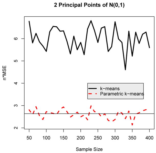
Plot of n × MSE versus sample size for estimating two principal points of the N(0, 1) distribution using the nonparametric and the parametric k-means algorithms. The solid horizontal line represents the asymptotic value of n × MSE for the maximum likelihood estimators of two principal points.

The next illustration is again for the standard normal distribution, except this time k = 5 principal points will be estimated. Figure 2 shows the plot of n × MSE for the nonparametric and parametric k-means algorithm for sample sizes ranging from n = 50 to 400 in increments of ten. As Figure 2 shows, the parametric k-means algorithm is performing even more efficiently than the nonparametric k-means algorithm for estimating k = 5 principal points compared to k = 2 principal points shown in Figure 1. In particular, n × MSE is about three times greater for the nonparametric k-means compared to the parametric k-means for k = 5 for larger sample sizes. The reason for the bigger difference between the parametric and nonparametric k-means when k = 5 is that the nonparametric k-means algorithm is estimating more parameters (five cluster means compared to two cluster means). Because there are fewer points per cluster when k = 5 versus k = 2, the estimated cluster means are less stable. However, for the parametric k-means algorithm, only the mean x̄ and standard deviation s need to be estimated regardless of the number k of cluster means specified. Thus, as the number k of principal points increases, the nonparametric k-means algorithm will deteriorate in terms of efficiency compared to the parametric k-means algorithm.

Figure 2.

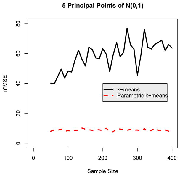
Plot of n × MSE versus sample size for estimating k = 5 principal points of the N(0, 1) distribution.

In order to illustrate the performance of the parametric k-means algorithm versus the nonparametric k-means algorithm for multivariate data, k = 2 principal points were estimated for a bivariate normal distribution with mean zero and a diagonal covariance matrix diag(σ², 1). The two principal points for this distribution lie along the first principal component axis (Tarpey et al. 1995) and are given by:

$$\left(\begin{array}{c}-\sqrt{2/\pi }\sigma \\ 0\end{array}\right)\hspace{0.17em}\text{and\hspace{0.17em}}\left(\begin{array}{c}\sqrt{2/\pi }\sigma \\ 0\end{array}\right).$$

Letting x̄ and S denote the sample mean and covariance matrix, the parametric k-means algorithm is run by simulating data from a N(x̄, S) distribution.

Because the two principal points must lie along the first principal component axis, we can modify the parametric k-means algorithm by constraining the cluster means to lie along the first sample principal component axis. The constrained principal point estimators are given by x̄ + β̂₁ξ̂_j for j = 1, …, k, where x̄ is the sample mean, β̂₁ is the eigenvector of the sample covariance matrix associated with the largest eigenvalue, and ξ̂₁, …, ξ̂_k are cluster means from the parametric k-means algorithm applied to the first principal component scores. Figure 3 shows a plot of n × MSE versus sample size for the nonparametric and parametric k-means algorithm along with the constrained method results using σ = 1.5. Once again, the parametric k-means performs more efficiently than the nonparametric k-means at all sample sizes. Also, the constrained method performs slightly more efficiently than the parametric k-means indicating a modest increase in efficiency. It would be interesting to extend the asymptotic results for the parametric k-means algorithm in Section 3 to the constrained parametric k-means algorithm.

Figure 3.

Plot of n × MSE for estimating two principal points of a bivariate normal distribution with covariance matrix diag(1.5², 1).

The performance of the parametric k-means algorithm depends on the validity of the parametric assumptions. For instance, suppose the parametric k-means algorithm is implemented assuming the data are from a bivariate normal distribution as above when in fact the true distribution is a bivariate t (Fang et al. 1990, page 85). A small scale simulation was performed to evaluate the performance of the misspecified parametric k-means algorithm in this situation for sample sizes ranging from 50 to 200, degrees of freedom ranging from 5 to 50, and for k = 2 and 5 principal points. In each case the parametric k-means algorithm based on the erroneous normality assumption performed much better than the nonparametric k-means algorithm with n × MSE being about 2 to 3 times greater for the nonparametric k-means algorithm compared to the parametric k-means algorithm, even for low degrees of freedom.

Another non-normal simulation was run using the chi-square distribution. k = 2 principal points were estimated for samples of sizes n = 25, 50, 75 and 100 using the nonparametric and parametric k-means algorithms. For the parametric k-means algorithm, a random sample of 100,000 was simulated from the correctly specified chi-square distribution with degrees of freedom equal to the sample mean. A parametric k-means algorithm was also run by misspecifying a normal distribution even though the true underlying distribution is chi-square. The simulation results, shown in Figure 4, were obtained for degrees of freedom ranging from 1 to 100 (horizontal axis). As expected, the correctly specified parametric k-means algorithm (long dashed curves) performs best. For large degrees of freedom, the chi-square is approximately normal and the misspecified parametric k-means based on the normal distribution (short-dashed curves) performs better than the nonparametric k-means algorithm (solid curves). For low degrees of freedom, the chi-square is very non-normal being strongly skewed to the right. In these cases the mis-specified parametric k-means algorithm either performs about the same as the nonparametric k-means for low sample sizes or performs slightly worse than the nonparametric k-means for larger sample sizes. For larger sample sizes, one should have the power to detect the non-normality (using a goodness-of-fit test for example) and therefore misspecifying a normal distribution for the parametric k-means algorithm can hopefully be avoided. However, for smaller sample sizes when it is more difficult to detect non-normality, the misspecified parametric k-means performs no worse than the nonparametric k-means algorithm.

Figure 4. Chi-Square Distribution.

n × MSE vs. degrees of freedom for the nonparametric k-means (solid curve), the correctly specified parametric k-means (long dashed curve); and the misspecified parametric k-means (short dashed curve). The four plots are for simulations using sample sizes n = 25, 50, 75 and 100.

5 Parametric k-Means Applied to Finite Mixtures

This section illustrates the parametric k-means algorithm in the setting of finite mixture distributions (see e.g. McLachlan and Krishnan 1997, Titterington et al. 1985) where closed form expressions do not typically exist for parameter estimates. Very little is known about principal points for mixture distributions. Yamamoto and Shinozaki (2000b) studied two principal points for the specialized case of a mixture of two spherically symmetric distributions. Determining principal points analytically for a mixture distribution is very difficult because of the wide variety of ways mixture distributions can be parameterized in terms of number of mixture components, mixing proportions, means and covariance structures of the mixture components.

In order to apply the parametric k-means algorithm, maximum likelihood estimation of the parameters of the mixture distribution are obtained via the EM algorithm (Dempster et al. 1977). Next, a very large sample size is simulated from a mixture distribution with parameters equal to the maximum likelihood estimates. In practice, one needs to specify the number of mixture components in order to run the EM algorithm. There have been numerous studies for determining the number of “groups” in a data set. A promising and simple approach is proposed by Sugar and James (2003) who also provide a review of many other methods of determining the number of groups in a data set.

In principal point applications involving finite mixtures, the number of principal points required will often differ from the number of mixture components. For example, suppose helmets are to be used for men and women and k different sizes need to be determined. The full population consists of two mixture components (males and females) but more than two sizes may be needed. In these types of applications, the number of mixture components is known and does not need to be determined. In fact, if the data identify who is male and who is female, then the EM algorithm is not needed to estimate the parameters of the two mixture components.

On the other hand, consider a clinical trial where quadratic curves are used to model longitudinal responses and the shape of the curve is clinically meaningful. Suppose the population is a mixture of two components: those who do and do not experience a placebo response. Membership in the two mixture components is not directly observed. Even if the distribution within each mixture component is homogeneous (e.g. normal), there will often be more than one representative response curve for individual components. For instance, if the degree of the responses (weak to strong) and the timing of the responses (immediate to delayed) vary according to a normal distribution, then the resulting response curves can take a variety of different shapes (e.g. see Tarpey et al. 2003).

Our first illustration is to estimate k = 4 principal points of a univariate normal mixture consisting of two components:

$$f(y)={\pi }_1{f}_1(y)+{\pi }_2{f}_2(y),$$

where the prior probabilities are both set equal to a half: π₁ = π₂ = 1/2, f₁ and f₂ are univariate normal distributions with unit variance and means μ₁ and μ₂ respectively. Figure 5 shows the results for three different mixtures. In each case μ₂ = 0 and μ₁ takes values 6, 4 and 3 for the three plots. In other words, the two mixture components are moving closer together from top to bottom of Figure 5. The plots on the left in Figure 5 show the mixture densities along with k = 4 principal points. The plots on the right show the corresponding n × MSE for the parametric and nonparametric k-means algorithm. To implement the parametric k-means algorithm, the EM algorithm was run on the data to obtain estimates of the prior probabilities π̂₁ and π̂₂ and the parametric simulation sample size (n_s = 100, 000) was split in two according to these estimated prior probabilities.

Figure 5.

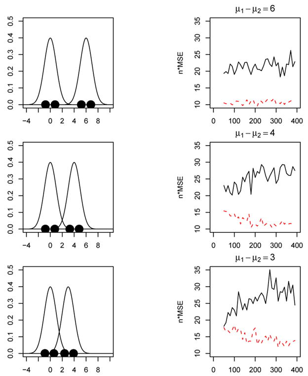
k = 4 principal points for a 2-component univariate normal mixture. Left panels: mixture densities with k = 4 principal points. Right panels: n × MSE versus sample size for the nonparametric (solid curve) and parametric k-means (dashed curve) algorithms.

For the plots at the top of Figure 5, the two mixture components are well separated (μ₁ − μ₂ = 6) and the parametric k-means algorithm performs much more efficiently than the nonparametric k-means for all sample sizes. In particular, the MSE for the nonparametric k-means is about twice as big as the MSE for the parametric k-means algorithm. It is interesting to note that the parametric k-means in this case performs much more efficiently than the nonparametric k-means although the parametric k-means requires estimating the mixture components via the EM algorithm. In this first case (top panels in Figure 5), the EM algorithm has an easy job because the mixture components are well separated. For the plots in the middle and at the bottom in Figure 5, the mixture components are closer together which makes it more difficult for the EM algorithm to accurately estimate the mixture components, especially for small sample sizes. The bottom right plot in Figure 5 shows that the parametric and nonparametric k-means perform about the same in terms of MSE for smaller sample sizes but as the sample size increases the parametric k-means outperforms the nonparametric k-means algorithm. In particular, once the sample size exceeds n = 170 the parametric k-means is about twice as efficient than the nonparametric k-means when the mixture component means differ by 3 (bottom plots in Figure 5).

Next the nonparametric and parametric k-means algorithms are compared for a bivariate normal mixture consisting of two components. For this illustration, k = 4 principal points are estimated from a mixture of two bivariate normal distributions with equal prior probabilities. The first component is centered at the origin with covariance matrix diag(2, 1) and the second component is centered at the point (7, 1) and the covariance matrix has eigenvalues 2 and 1, similar to the first component, but the distribution has been rotated by π/3 radians. Figure 6 shows a picture of this mixture distribution by plotting the elliptical contours of equal density for each component as well as k = 4 principal points. Implementing the parametric k-means algorithm for a multivariate mixture distribution introduces some added complexity. As in the univariate case, the parameters of the mixture components are estimated using the EM algorithm. Simulating from the estimated mixture distribution in the multivariate case requires simulating the correct covariance structure for each mixture component which requires extracting the eigenvalues and vectors from the covariance matrices estimated from the EM algorithm. Figure 7 shows a plot of n × MSE versus sample size for the non-parametric and parametric k-means. Once again, the parametric k-means is about twice as efficient as the nonparametric k-means.

Figure 6.

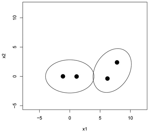
k = 4 principal points for a mixture of two bivariate normal distributions with equal priors. One component is centered at the origin with covariance matrix diag(2,1). The other component is obtained from the first component by centering it at the point (7,1) and rotating the distribution by π/3 radians.

Figure 7.

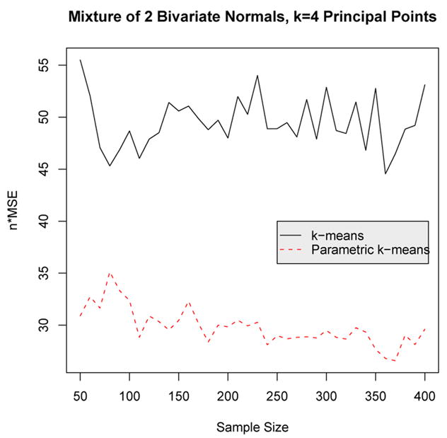
n × MSE versus sample size for the nonparametric and parametric k-means algorithm for a mixture of two bivariate normal distributions with k = 4 principal points.

6 Example

Flury (1990) coined the term principal points in the problem of determining optimal sizes and shapes of protection masks for men in the Swiss army. For example, estimating k = 3 principal points would be useful for determining a small, medium and large size mask. p = 6 head dimension variables were measured on a sample of n = 200 men: minimal frontal breadth (MFB), breadth of angulus mandibulae (BAM), true facial height (TFH), length from glabella to apex nasi (LGAN), length from tragion to nasion (LTN), and length from tragion to gnathion (LTG) (Flury 1997, page 8).

The Swiss head dimension data appears consistent with a multivariate normal distribution (Flury 1990) and thus the parametric k-means algorithm will be used assuming the distribution is multivariate normal. Without using the parametric k-means algorithm, it would be extremely difficult to determine k > 4 principal points of a p = 6 dimensional multivariate normal distribution.

In order to compare the performance of the nonparametric and parametric k-means algorithm, a leave-one-out prediction error was computed for different values of k. The leave-one-out prediction error was computed by leaving out a single data point and then estimating the k principal points using both the nonparametric and parametric k-means algorithms. The squared distance between the left-out point to the nearest estimated cluster mean was then computed. This was repeated for all observations and the average squared error, called the Prediction Mean Squared Error (PMSE) was computed. For each leave-one-out iteration, estimated cluster centers from the full data set were used as starting seeds for the k-means algorithm so the problem of multiple stationary points was minimized. 500,000 simulated observations were used in the parametric k-means algorithm. The results, summarized in Figure 8, show that the parametric k-means algorithm is superior to the nonparametric k-means algorithm for all values of k = 2, …, 8, although the difference between the two methods is rather small for k = 5, 6 and 7 which may be attributable to slight departures from normality in the data.

Figure 8.

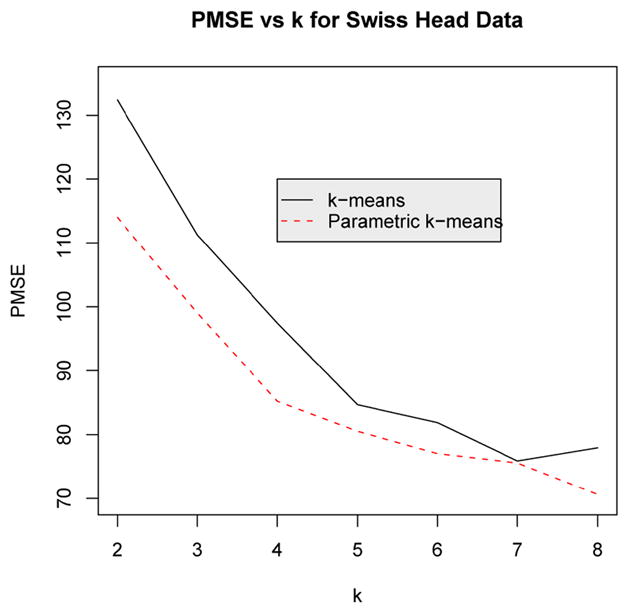
Plot of the leave-one-out prediction error (PMSE) comparing the parametric (dashed curve) and the usual nonparametric k-means algorithm for the p = 6 dimensional Swiss head data for values of k = 2, 3, …, 8.

The computation time required to implement the parametric k-means algorithm for this example is modest. It took about 3 seconds to implement the parametric k-means using a simulated sample size of 500,000 in this example for k = 2 and about 15 seconds for k = 8 on a pentium 1.79GHz machine. The time required for the leave-one-out PMSE computations can be computed by multiplying these times by the sample size n, in this case n = 200. More complicated models, like finite mixture models, would require additional time to get the initial parameter estimates for the parametric k-means simulation.

A Self-Consistency Test

For the Swiss head data we assumed the distribution is multivariate normal when implementing the parametric k-means algorithm. The validity of the normality assumption can be assessed by evaluating the self-consistency of the parametric k-means solution. From the definition of self-consistent points in Section 1 it follows that each estimated principal point from the parametric k-means algorithm should be approximately equal to the average of the original data points that are closest to the principal point. To illustrate, Figure 9 shows k = 6 estimated principal points (large solid circles) for the Swiss head dimension data estimated using the parametric k-means algorithm and projected into the subspace of the first two principal components. The k = 6 points form a pentagon pattern with a center point. Let ξ̂_j denote an estimated principal point (j = 1,…, k) and let x̄_j denote the average of the original Swiss head data points closest to ξ̂_j. The x̄_j are plotted by the large open circles in Figure 9. The self-consistency condition stipulates that ξ̂_j ≈ x̄_j for j = 1 …, k. If the data deviates strongly from normality, then the parametric k-means estimators of principal points should fail to be self-consistent points for the data. In order to access the self-consistency condition, we can form the test statistic:

Figure 9.

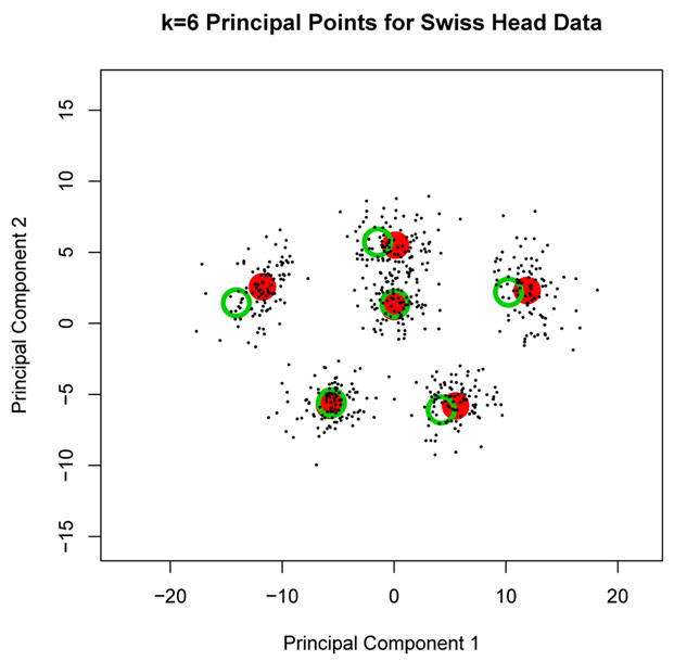
k = 6 principal points (large solid circles) for the Swiss head dimension data estimated using the parametric k-means algorithm and projected into the subspace of the first two principal components. The large open circles are the sample means of the Swiss data over the regions formed by partitioning the data into clusters formed by the k = 6 principal points. The small dots are the corresponding cluster means from 100 simulated N(x̄, S) data sets.

$$T^2=\sum _{j=1}^k\parallel {\widehat{\mathit{\xi }}}_j-{\overline{\mathit{x}}}_j{\parallel }^2.$$ (8)

An approximate test of significance can be performed by evaluating T² under the null hypothesis that the data is from a normal distribution by the following steps:

1. Simulate N samples of size n from a N(x̄, S) distribution where x̄ and S are the sample mean and covariance matrix of the original data;

2. Estimate k-principal points using the parametric k-means algorithm for each simulated sample;

3. Compute T² in (8) for each simulated sample; and

4. Compute a p-value as the proportion of simulated T²’s exceeding the T² for the original data.

This self-consistency test was run on the Swiss head data using k = 6. The p-value (estimated using N = 100) is p = 0.51 indicating that there is no evidence against self-consistency of the k = 6 principal point estimates from the parametric k-means algorithm solution for the Swiss head data. The small solid circles in Figure 9 correspond to the sample means x̄_j for N = 100 data sets simulated from N(x̄, S). It is evident from Figure 9 that the differences between the large solid and open circles (the ξ̂_j and x̄_j) is consistent with the variability one would expect to see with actual normal data since the large open circles fall within the cloud of points formed by the small solid circles. The self-consistency test was also run for other values of k = 2, …, 8 for the Swiss head data (using N = 100) yielding p-values p = 0.81, 0.83, 0.47, 0.35, 0.51, 0.63, and 0.70 respectively indicating that there is no evidence against self-consistency of the principal point estimates from the parametric k-means algorithm.

R-code for implementing the parametric k-means algorithm for a multivariate normal distribution and the self-consistency test can be found at:

http://www.math.wright.edu/People/Thad_Tarpey/thad.htm.

Head dimension data was also available for n = 59 females. Combining the male and female data would allow for determining sizes that could be used by both sexes. This is analogous to a mixture distribution, except individual data points were identified as male or female, so the EM algorithm was not needed to estimate parameters for males and females separately. The nonparametric and parametric k-means algorithms were compared again in terms of PMSE for the combined data and essentially both methods performed about the same. The reason the parametric k-means did not perform consistently better than the nonparametric k-means algorithm in this example is because the distribution for some of the variables for the females deviated from normality. This illustrates that the optimality of the parametric k-means algorithm depends on the validity of the parametric assumptions.

7 Discussion

Before powerful computing was readily available, determining optimal point representations or optimal partitions of theoretical distributions was severely limited. The computer intensive parametric k-means algorithm illustrated in this paper provides an almost effortless method of determining and estimating principal points with maximum likelihood efficiency. The simulation results in Section 4 demonstrate that the parametric k-means algorithm can be considerably more efficient than the usual nonparametric k-means algorithm.

The performance of the parametric k-means algorithm depends on the validity of the parametric assumptions. Section 4 reported some preliminary results on the performance of the parametric k-means algorithm when the specified distribution (e.g. normal) differs from the true distribution. It would be useful to perform an in depth investigation into the robustness of the parametric k-means algorithm in the presence of outliers and other deviations from parametric assumptions. It would also be useful to evaluate the performance of the parametric k-means algorithm for high dimensional data. However, for moderate values of k that tend to be used in practice, the space spanned by k principal points will often tend to be low dimensional (Tarpey et al. 1995).

The Swiss head dimension data was used to illustrate the parametric k-means algorithm in Section 6 since that was the original example that motivated the term principal points. However, the motivation for this current work was the problem of clustering functional data (Abraham et al. 2003, James and Sugar 2003, Luschgy and Pagés 2002, Tarpey and Kinateder 2003) where different cluster means can be used to identify representative curve shapes in the data. It is anticipated that the parametric k-means algorithm will be very useful in these types of applications due to the high dimensional nature of the data.

References

- Abraham C, Cornillon PA, Matzner-Lober E, Molinari N. Unsupervised curve clustering using B-splines. Scandinavian Journal of Statistics. 2003;30:1–15. [Google Scholar]
- Connor R. Grouping for testing trends in categorical data. Journal of the American Statistical Association. 1972;67:601–604. [Google Scholar]
- Cox DR. A note on grouping. Journal of the American Statistical Association. 1957;52:543–547. [Google Scholar]
- Dalenius T. The problem of optimum stratification. Skandinavisk Aktuarietidskrift. 1950;33:203–213. [Google Scholar]
- Dalenius T, Gurney M. The problem of optimum stratification ii. Skandinavisk Aktuarietidskrift. 1951;34:133–148. [Google Scholar]
- Dempster AP, Laird NM, Rubin DB. Maximum likelihood from incomplete data via the EM algorithm. Journal of the American Statistical Association. 1977;39:1–38. [Google Scholar]
- Eubank RL. Optimal grouping, spacing, stratification, and piecewise constant approximation. Siam Review. 1988;30:404–420. [Google Scholar]
- Fang K, He S. The problem of selecting a given number of representative points in a normal population and a generalized mill’s ratio. Technical report, Department of Statistics; Stanford University: 1982. [Google Scholar]
- Fang KT, Kotz S, Ng KW. Symmetric Multivariate and Related Distributions. Chapman and Hall; London: 1990. [Google Scholar]
- Flury B. Principal points. Biometrika. 1990;77:33–41. [Google Scholar]
- Flury B. Estimation of principal points. Applied Statistics. 1993;42:139– 151. [Google Scholar]
- Flury B. A First Course in Multivariate Statistics. Springer; New York: 1997. [Google Scholar]
- Flury BD, Tarpey T. Representing a large collection of curves: A case for principal points. The American Statistician. 1993;47:304–306. [Google Scholar]
- Graf L, Luschgy H. Foundations of Quantization for Probability Distributions. Springer; Berlin: 2000. [Google Scholar]
- Gu XN, Mathew T. Some characterizations of symmetric two-principal points. Journal of Statistical Planning and Inference. 2001;98:29–37. [Google Scholar]
- Hand DJ, Krzanowski WJ. Optimising k-means clustering results with standard software packages. Computational Statistics & Data Analysis. 2005;49:969–973. [Google Scholar]
- Hartigan JA. Clustering Algorithms. Wiley; New York: 1975. [Google Scholar]
- Hartigan JA, Wong MA. A k-means clustering algorithm. Applied Statistics. 1979;28:100–108. [Google Scholar]
- Iyengar S, Solomon H. Recent Advances in Statistics: Papers in Honor of Herman Chernoff on his 60th Birthday. Academic Press; 1983. Selecting representative points in normal populations; pp. 579–591. [Google Scholar]
- James G, Sugar C. Clustering for sparsely sampled functional data. Journal of the American Statistical Association. 2003;98:397–408. [Google Scholar]
- Li L, Flury B. Uniqueness of principal points for univariate distributions. Statistics and Probability Letters. 1995;25:323–327. [Google Scholar]
- Luschgy H, Pagés G. Functional quantization of Gaussian processes. Journal of Functional Analysis. 2002;196:486–531. [Google Scholar]
- MacQueen J. Some methods for classification and analysis of multivariate observations. Proceedings 5th Berkeley Symposium on Mathematics, Statistics and Probability. 1967;3:281–297. [Google Scholar]
- McLachlan GJ, Krishnan T. The EM Algorithm and Extensions. Wiley; New York: 1997. [Google Scholar]
- Mease D, Nair VN, Sudjianto A. Selective assembly in manufacturing: Statistical issues and optimal binning strategies. Technometrics. 2004;46:165–175. [Google Scholar]
- Pollard D. Strong consistency of k-means clustering. Annals of Statistics. 1981;9:135–140. [Google Scholar]
- Pollard D. A central limit theorem for k-means clustering. Annals of Probability. 1982;10:919–926. [Google Scholar]
- Pötzelberger K, Felsenstein K. An asymptotic result on principal points for univariate distributions. Optimization. 1994;28:397–406. [Google Scholar]
- R Development Core Team. R: A language and environment for statistical computing. R Foundation for Statistical Computing; Vienna, Austria: 2003. [Google Scholar]
- Ramsay JO, Silverman BW. Functional Data Analysis. Springer; New York: 1997. [Google Scholar]
- Rowe S. An algorithm for computing principal points with respect to a loss function in the unidimensional case. Statistics and Computing. 1996;6:187–190. [Google Scholar]
- Stampfer E, Stadlober E. Methods for estimating principal points. Communications in Statistics|Series B, Simulation and Computation. 2002;31:261–277. [Google Scholar]
- Su Y. On the asymptotics of qunatizers in two dimensions. Journal of Multivariate Analysis. 1997;61:67–85. [Google Scholar]
- Sugar C, James G. Finding the number of clusters in a data set: An information theoretic approach. Journal of the American Statistical Association. 2003;98:750–763. [Google Scholar]
- Tarpey T. Two principal points of symmetric, strongly unimodal distributions. Statistics and Probability Letters. 1994;20:253–257. [Google Scholar]
- Tarpey T. Principal points and self–consistent points of symmetric multivariate distributions. Journal of Multivariate Analysis. 1995;53:39–51. [Google Scholar]
- Tarpey T. Estimating principal points of univariate distributions. Journal of Applied Statistics. 1997;24:499–512. [Google Scholar]
- Tarpey T. Self-consistent patterns for symmetric multivariate distributions. Journal of Classification. 1998;15:57–79. [Google Scholar]
- Tarpey T, Flury B. Self–consistency: A fundamental concept in statistics. Statistical Science. 1996;11:229–243. [Google Scholar]
- Tarpey T, Kinateder KJ. Clustering functional data. Journal of Classification. 2003;20:93–114. [Google Scholar]
- Tarpey T, Li L, Flury B. Principal points and self–consistent points of elliptical distributions. Annals of Statistics. 1995;23:103–112. [Google Scholar]
- Tarpey T, Petkova E, Ogden RT. Profiling placebo responders by self-consistent partitions of functional data. Journal of the American Statistical Association. 2003;98:850–858. [Google Scholar]
- Titterington DM, Smith AFM, Makov UE. Statistical Analysis of Finite Mixture Distributions. Wiley; New York: 1985. [Google Scholar]
- Wei GCG, Tanner MA. A monte carlo implementation of the EM algorithm and the poor man’s data augmentation algorithms. Journal of the American Statistical Association. 1990;85:699–704. [Google Scholar]
- Yamamoto W, Shinozaki N. On uniqueness of two principal points for univariate location mixtures. Statistics & Probability Letters. 2000a;46:33–42. [Google Scholar]
- Yamamoto W, Shinozaki N. Two principal points for multivariate location mixtures of spherically symmetric distributions. Journal of the Japan Statistical Society. 2000b;30:53–63. [Google Scholar]
- Zoppé A. Principal points of univariate continuous distributions. Statistics and Computing. 1995;5:127–132. [Google Scholar]
- Zoppé A. On uniqueness and symmetry of self-consistent points of univariate continuous distributions. Journal of Classification. 1997;14:147–158. [Google Scholar]