Computational neural network analysis of the affinity of lobeline and tetrabenazine analogs for the vesicular monoamine transporter-2

Abstract

Back-propagation artificial neural networks (ANNs) were trained on a dataset of 104 VMAT2 ligands with experimentally measured log(1/K_i) values. A set of related descriptors, including topological, geometrical, GETAWAY, aromaticity, and WHIM descriptors was selected to build nonlinear quantitative structure-activity relationships. A partial least squares (PLS) regression model was also developed for comparison. The nonlinearity of the relationship between molecular descriptors and VMAT2 ligand activity was demonstrated. The obtained neural network model outperformed the PLS model in both the fitting and predictive ability. ANN analysis indicated that the computed activities were in excellent agreement with the experimentally observed values (r² = 0.91, rmsd = 0.225; predictive q² = 0.82, loormsd = 0.316). The generated models were further tested by use of an external prediction set of 15 molecules. The nonlinear ANN model has r² = 0.93 and root-mean-square errors of 0.282 compared with the experimentally measured activity of the test set. The stability test of the model with regard to data division was found to be positive, indicating that the generated model is predictive. The modeling study also reflected the important role of atomic distribution in the molecules, size, and steric structure of the molecules when they interact with the target, VMAT2. The developed models are expected to be useful in the rational design of new chemical entities as ligands of VMAT2 and for directing synthesis of new molecules in the future.

1. Introduction

Methamphetamine (METH), an amphetamine derivative, is an addictive psychostimulant drug and a significant health concern due to its abuse liability and potential neurotoxic effects.¹ Chronic use of METH may cause long-term neural damage in humans, with concomitant deleterious effects on cognitive processes, such as memory and attention.² Despite the serious consequences of METH abuse, currently there is no FDA approved clinical treatment for METH addiction. Thus, there is an increasing interest in identifying the underlying mechanisms of METH action, as well as the relevant pharmacological targets to promote the development of novel therapeutic agents as treatments for METH abuse.

The abuse liability of METH and structurally-related amphetamine compounds is thought to be due to alterations in dopaminergic neurotransmission.^3,4 In this respect, the dopamine transporter (DAT) and the vesicular monoamine transporter-2 (VMAT2), presynaptic proteins critical for dopamine storage and release, are the primary targets for METH action.^3,4,5 Specifically, METH interacts with VMAT2 to release dopamine from the synaptic vesicles into the cytosol of the presynaptic terminal,^6,7 METH also inhibits monoamine oxidase and evokes the release of dopamine from the cytosol into the extracellular space via reverse transport of DAT, leading to an increase in dopamine concentration in the extracellular space.^7,8,9

Lobeline, an alkaloidal constituent of Lobelia inflata LINN, is a nicotinic receptor ligand with high affinity for α4β2* nicotinic receptors.¹⁰ Lobeline was previously investigated as a therapeutic agent to treat tobacco dependence.¹⁰ Recent study indicated that lobeline has both temperature-dependent and temperature-independent neuroprotective effects against METH toxicity.¹¹ Lobeline also inhibits dopamine uptake and promotes dopamine release from storage vesicles within the presynaptic terminal via an interaction with the tetrabenazine binding site on VMAT2.¹² Lobeline attenuates d-amphetamine- and methamphetamine-induced hyperactivity, and inhibits the discriminative stimulus effects and self-administration of methamphetamine.^13,14 However, lobeline does not support self-administration in rats,¹⁵ suggesting a lack of addiction liability. Thus, the development of lobeline and lobeline analogs with targeted selectivity at VMAT2, represents a novel approach for the treatment for psychostimulant abuse.^{10, 12}

To date, very few VMAT2 ligands have been reported in the literature; these include low affinity ligands, such as 3-amino-2-phenylpropene derivatives,¹⁶ and high affinity tetrabenazine derivatives.^17,18 Tetrabenazine was introduced in 1956 as an antipsychotic agent ¹⁹ and has currently been submitted for FDA approval as an anti-chorea drug.²⁰ Recently, a small library of structural analogs of lobeline have been synthesized, and their activity and selectivity for VMAT2 have been evaluated.^9,21,22,23

In the discovery of novel and more potent and selective lobeline analogs, we consider computational modeling as a valuable aid in drug design and optimization. In this respect, the nature of the interaction of these novel ligands with the binding site(s) on VMAT2 is not known due to the lack of crystal structure for this protein. Thus, a structure-based drug design approach is not available. On the other hand, neural network analysis approach, particular back-propagation network to data analysis, has received much attention over last decade. This artificial system emulates the function of the brain, in which a very high number of information-processing neurons are interconnected and are known for their ability to model a wide set of functions, including linear and non-linear functions, without knowing the analytic forms in advance.²⁴ The rapid advancement of computing systems in the past 20 years is an important factor leading to the success of this approach in various engineering, business, and medical applications. So far, the neural network approach has been applied in a variety of biomedical areas, which includes analysis of appendicitis²⁵ and cancer imaging extraction and classification,²⁶ AIDS research and therapy.²⁷ This approach has also been used in drug design and discovery;²⁴ as well as in pharmaceutical applications such as pharmaceutical production development,²⁸ pharmacodynamic modeling²⁹ and mapping dose-effect relationships on pharmacological response.³⁰

In this current study, the neural network analysis approach is used to build a quantitative structure-activity relationship (QSAR) model on a set of 104 tetrabenazine and lobeline analogs with known affinity for VMAT2. This is the first QSAR modeling study that addresses the interaction of a small library of ligands at the VMAT2 binding site. The goals of the current work are (i) to extract the relevant descriptors to establish the QSAR of the library of ligands, (ii) to establish the high predictive power of neural network modeling on this library of compounds, and (iii) to develop insights regarding the relationship between the descriptors of the compounds and their affinity for VMAT2. The developed models are expected to be valuable in the rational design of chemical modifications of first-generation VMAT2 ligands in order to identify the most likely candidates for synthesis and discovery of new lead compounds.

2. Methods

2.1 Generation of the molecular database

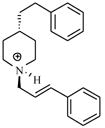
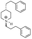
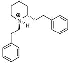
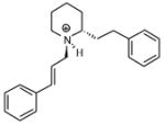
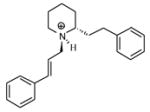
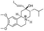
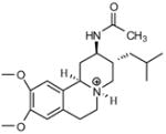
Molecular modeling was carried out with the aid of the Sybyl discovery software package.^31a The software was used to construct the initial molecular structures utilized in the geometry optimization (energy minimization) for all molecules evaluated in this study. The geometry optimization was first performed by using the molecular mechanics (MM) method with the Tripos force field and the default convergence criterion. Since the pK_a values of the basic nitrogen atoms in these compounds are between 8 and 10, and the synaptic vesicles are acidic (pH 5-5.6)³², most microspecies of the compounds are expected to be protonated when binding to VMAT2³³. Thus, in the construction of the initial molecular structures, the basic nitrogen atoms in these compounds were protonated with a formal charge of +1 assigned to the positively charged nitrogen atom. In this respect, the crystal structures of meso-transdiene (MTD, compound T78 in Table 1) shown in Figure 1, the structure of lobeline in crystal structure of acetylcholine-binding protein from aplysia californica in complex with lobeline (PDB code 2BYS), and the crystal structure of (−)-α-9-O-desmethyldihydro- tetrabenazine^34a were utilized as a reference. It has been shown that only the (+)-isomer of dihydrotetrabenazine exhibited high affinity for VMAT2.^34b Protonation of nitrogen atom in these molecules is also relevant, considering that some of the lobeline analogs in the dataset include quaternary ammonium nitrogen atoms, such as T6, P6 and P7 in Table 1. All of the obtained conformations optimized at the MM level were further refined to their lowest energy states with MOPAC, a semi-empirical molecular modeling routine, utilizing the PM3 Hamiltonian.

Table 1.

Structures, experimental log(1/K_i ) values (K_i values are expressed as molar), and log(1/K_i) values calculated by the trained NN11-3-1 and PLS models, and their leave-one-out (LOO) validation results

Compound	Structure	log(1/Ki) (Expt.)	log(1/Ki) (NN)	log(1/Ki) (NNLOO)	log(1/Ki) (PLS)	log(1/Ki) (PLSLOO)
P1		5.89	5.61		5.84
P2		5.40	5.25		5.34
T1		5.86	5.91	5.89	5.78	5.52
P3		5.32	5.38		5.87
T2		5.41	5.47	5.54	5.92	6.04
T3		5.19	5.46	5.54	5.42	5.43
T4		5.29	5.36	5.36	5.34	5.39
T5		5.22	5.43	5.45	5.32	5.35
P4		5.60	5.38		5.54
T6		5.28	5.23	5.24	5.30	5.35
T7		5.03	4.95	5.00	4.96	4.95
P5		5.70	5.51		5.52
T8		5.52	5.55	5.53	5.48	5.55
T9		5.51	5.58	5.59	5.39	5.42
T10		5.57	5.49	5.46	5.67	5.69
T11		5.27	5.18	5.21	5.26	5.28
P6		4.78	5.22		5.64
T12		5.15	5.24	5.24	5.24	5.19
T13		5.19	5.18	5.14	5.41	5.48
T14		5.64	5.40	5.36	5.53	5.55
P7		4.61	5.12		5.17
T15		5.63	5.68	5.59	5.63	5.55
T16		6.28	6.17	5.96	5.93	5.78
T17		5.48	5.58	5.62	5.69	5.80
T18		5.76	5.92	5.92	5.68	5.82
T19		5.49	5.52	5.52	5.34	5.34
T20		5.36	5.55	5.66	5.25	5.28
P8		5.90	5.59		5.75
T21		6.01	5.95	5.96	5.88	5.86
T22		5.52	5.52	5.19	5.50	5.52
T23		5.33	5.61	5.81	5.73	5.68
P9		6.20	5.78		5.68
T24		5.88	5.85	5.82	5.76	5.73
T25		5.98	6.14	6.38	6.12	6.16
T26		5.78	5.66	5.64	6.06	6.15
T27		6.37	5.83	5.70	6.00	6.08
T28		5.42	5.38	5.35	5.53	5.51
P10		5.00	5.21		5.63
T29		5.82	5.83	5.87	5.69	5.64
T30		5.69	5.45	5.26	5.42	5.30
T31		5.23	5.19	5.68	6.00	6.20
T32		5.32	5.42	5.98	5.52	5.62
T33		5.28	5.47	5.72	5.47	5.62
T34		5.68	5.32	5.27	5.17	5.12
T35		5.29	5.40	5.40	5.39	5.38
T36		4.97	4.93	5.17	5.38	5.47
T37		5.73	5.81	5.86	5..60	5.68
T38		6.24	6.00	5.90	5.46	5.36
T39		5.80	5.58	5.50	5.48	5.48
T40		5.97	6.13	6.11	5.52	5.45
T41		5.80	5.74	5.84	5.80	5.80
T42		6.24	5.99	5.91	5.98	5.96
P11		5.47	5.57		5.79
T43		5.73	5.81	6.02	5.74	5.78
T44		5.21	5.41	5.40	5.32	5.33
P12		5.06	4.78		5.28
T45		4.93	5.37	5.43	5.23	5.26
T46		5.03	5.00	4.95	5.22	5.17
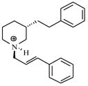
T47		4.98	5.39	5.43	5.15	5.18
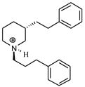
T48		5.39	5.37	5.39	5.17	5.17
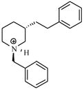
T49		5.02	4.96	4.98	5.40	5.36
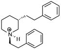
T50		5.40	5.43	5.43	5.34	5.30
T51		4.89	5.02	5.15	5.36	5.28
T52		4.85	5.01	5.02	5.38	5.41
T53		5.73	5.46	5.41	5.68	5.63
T54		5.48	5.71	5.80	5.36	5.36
T55		5.61	5.82	5.95	5.49	5.51
T56		5.48	5.41	5.39	5.33	5.38
T57		5.51	5.58	5.59	5.30	5.35
T58		5.48	5.30	5.27	5.29	5.33
T59		4.43	4.75	4.95	4.88	4.98
T60		5.21	5.08	4.69	4.95	4.88
T61		4.85	5.21	5.29	5.32	5.37
T62		5.87	5.46	5.40	5.44	5.37
T63		5.58	5.23	5.19	5.34	5.33
T64		5.28	5.42	5.43	5.42	5.44
T65		6.23	5.53	5.51	5.23	5.19
T66		5.18	5.62	5.71	5.54	5.63
T67		5.40	5.57	5.66	5.32	5.45
T68		5.39	5.40	5.52	5.53	5.55
T69		5.51	5.20	5.12	5.14	5.10
T70		5.66	5.63	5.63	5.66	5.57
T71		6.01	5.31	5.24	5.79	5.83
T72		4.88	5.25	5.34	5.43	5.54
T73		5.49	5.45	5.47	5.46	5.38
T74		5.56	5.56	5.59	5.53	5.53
T75		5.00	5.32	5.36	5.35	5.36
T76		5.15	5.03	5.01	5.23	5.18
T77		5.15	5.25	5.26	5.03	5.49
T78		5.47	5.46	5.07	5.03	4.77
T79		4.76	4.84	4.85	5.19	5.16
T80		4.60	4.71	4.72	4.51	4.35
T81		7.89	8.31	8.40	7.98	7.93
P13		7.55	7.63		7.87
T82		8.59	8.22	8.05	7.87	7.73
T83		7.92	8.02	8.01	7.96	7.94
P14		7.70	8.00		7.69
T84		7.08	7.27	7.40	7.41	7.49
T85		6.87	7.04	7.43	7.16	7.27
T86		7.48	7.24	7.13	7.04	7.01
P15		8.12	8.11		7.79
T87		7.59	7.57	7.52	7.76	7.90
T88		7.49	7.55	7.21	7.35	7.07
T89		6.14	6.10	6.21	6.31	6.34

Figure 1.

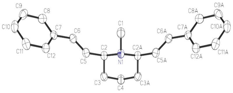
Crystal structure of meso-transdiene (MTD).

The 104 molecules listed in Table 1 constitute a database for the structure-activity relationship analysis. These data are a combination of 10 previously reported compounds with experimental K_i values,^17,18 and 94 compounds with experimental K_i values from our own laboratory.^9,21–23 A dataset of 89 molecules (T1–T89) was used for model training and leave-one-out (LOO) validation. A dataset of 15 molecules (P1–P15) from a different compound series was used for external testing. Table 1 also lists the experimental K_i values for each of these compounds, providing the pharmacological parameter which characterizes the interaction with the VMAT2 binding site. For the set of the 104 molecules utilized, the K_i values of 13 molecules were ≤ 0.01 μM, 10 molecules had K_i values in the range 0.1–1 μM, 63 molecules had K_i values in the range 1–10 μM, and 14 molecules had K_i values ≥ 10 μM.

2.2 Generation of molecular descriptors

The optimum three-dimensional conformations were used for generation of descriptors, some of which were geometry-dependent. A total of 807 molecular descriptors, consisting of zero-dimensional (constitutional descriptors), one-dimensional (functional groups, empirical descriptors, physical properties), two-dimensional (topological descriptors), as well as three-dimensional (geometrical, WHIM, GETAWAY, aromaticity descriptors) variables, were created by the DRAGON program.^35a A reduced set of 149 descriptors was obtained after the constant and near constant descriptors and the highly inter-correlated (>0.95) descriptors were discarded.

2.3 Partial least squares regression analysis

Partial least squares (PLS) analysis was performed using the QSAR module of Sybyl version 7.0, with the NIPALS algorithm to extract the original variable into PLS components. All variables were initially auto-scaled to zero mean and unit variance. This method produces new variables by a linear combination of the original descriptors and uses them to predict the biological activities. The advantage of this method is that the method can be used for strongly correlated, noisy data with numerous independent variables (e.g. in modeling data sets where the number of descriptors greatly exceeds the number of observations).³⁶

2.4 Target properties

Experimental K_i values of lobeline and its analogs were measured according to the procedure described by Zheng et al.⁹ Experimental K_i values of tetrabenazine and its analogs, except for tetrabenazine and Ro4-1284 (P13 and P14 in Table 1 respectively) were taken from Lee et al.¹⁷ and Conney et al.¹⁸ The K_i values for tetrabenazine and Ro4-1284 were also measured in our laboratory to compare the K_i values with those from the other laboratories. The K_i values for P13 and P14 obtained from our own assays (0.013 μM and 0.028 μM, respectively) were used in this study. These K_i values are very similar to the literature values for these compounds (i.e., 0.0081 μM and 0.042 μM, respectively) reported by Lee et al.¹⁷ Conney et al. ¹⁸ also reported a K_i value of 0.0067 μM for tetrabenazine. The log(1/K_i), with K_i values expressed as molar, was used as the target pharmacological criterion to derive the QSARs.

2.5 ANN QSAR modeling

Feed-forward, back-propagation-of-error networks were developed using a neural network C program.³⁷ Network weights (W_ji(s)) for a neuron “j” receiving output from neuron “i” in the layer “s” were initially assigned random values between −0.5 and +0.5. The sigmoidal function was chosen as the transfer function that generates the output of a neuron from the weighted sum of inputs from the preceding layer of units. Consecutive layers were fully interconnected; there were no connections within a layer or between the input and the output. A bias unit with a constant activation of unity was connected to each unit in the hidden and output layers.

The input vector was the set of descriptors for each molecule in the series, as generated by the previous steps. All descriptors and targets were normalized to the [0,1] interval using the following formula:

$${X_{ij}}^{\prime }=\frac{X_{ij}-X_j{,}_{min}}{X_j{,}_{max}-X_j{,}_{min}}$$ (1)

Where X_ij and X_ij′ represents the original value and the normalized value of the j-th (j=1,…k) descriptor for compound i (i=1,…n). X_min and X_max represent the minimum and maximum values for the j-th descriptor. The network was configured with one or more hidden layers. During the ANN learning process, each compound in the training set was iteratively presented to the network. That is, the input vector of the chosen descriptors in normalized form for each compound was fed to the input units, and the network’s output was compared with the experimental “target” value. During one “epoch”, all compounds in the training set were presented, and weights in the network were then adjusted on the basis of the discrepancy between network outputs and observed log(1/K_i) values by back-propagation using the generalized delta rule.

2.6 Cross-validation and testing

Models were cross-validated using the “leave-one-out” approach.³⁸

Generated models were then tested using a subset of 15 compounds (P1–P15 in Table 1). They were randomly selected to cover the experimental activity range as uniformly as possible, and were not used in either the variable selection or the model building processes.

2.7 Evaluation of the QSAR models

QSAR models were assessed by Pearson correlation coefficient r², root mean square deviation (rmsd), and predictive q²_, which is defined as

$$q^2=\frac{SD-\mathit{PRESS}}{SD}$$ (2)

Where SD is the sum of squared deviations of each measured log(1/K_i) value from its mean, and PRESS is the sum of squared differences between actual and predicted values.

3. Results and Discussion

3.1 PLS analysis and neural network configuration

To provide a comparison with the neural network model, a linear PLS analysis was carried out on the affinity for the training set of 89 compounds. Variable selection from 149 descriptors generated as described in section 2.2 was used to build the PLS model. After stepwise exclusion of low contribution variables, 12 variables were included in the model, resulting in an equation in which only variables that significantly increased the predictability of the dependent variable were included. During the PLS analysis, five components (latent vectors) that explain the most covariance between the 12 descriptors and experimental log(1/K_i) values are obtained. The linear model built with these five components corresponds to the highest q² (0.780) and lowest LOO rmsd (0.353). A final set of 12 descriptors which gave the best PLS model is listed in Table 2.

Table 2.

Brief description of the descriptors used in the PLS and nonlinear neural network analyses

Descriptor	Definition	Typec
Ram a, b	Ramification index.	1
DISPp a	d COMMA2 value/weighted by atomic polarizabilities.	2
HATS5u a	Leverage-weighted autocorrelation of lag 5/unweighted.	3
R5u a	R autocorrelation of lag 5/unweighted.	3
R1v+ a	R maximal autocorrelation of lag 1/weighted by atomic van der Waals volumes.	3
R5v+ a	R maximal autocorrelation of lag 5/weighted by atomic van der Waals volumes.	3
R5e+ a	R maximal autocorrelation of lag 5/weighted by atomic Sanderson electronegativities.	3
R4u+ a	R maximal autocorrelation of lag 4/unweighted.	3
PW5 a, b	Path/walk 5-Randic shape index.	1
LP1 b	Lovasz-Pelikan index [leading eigenvalue].	1
SEige b	Eigenvalue sum from electronegativity weighted distance matrix.	1
VEp2 b	Average eigenvector coefficient sum from polarizability weighted distance matrix.	1
DISPm a, b	d COMMA2 value/weighted by atomic masses.	2
G(N..N)a, b	Sum of geometrical distances between N..N.	2
H7m b	H autocorrelation of lag 7/weighted by atomic masses.	3
RCON a, b	Randic-type R matrix connectivity.	3
R1p+ b	R maximal autocorrelation of lag 1/weighted by atomic polarizabilities.	3
HOMT b	HOMA (harmonic oscillator model of aromaticity index) total.	4
G1u b	1st component symmetry directional WHIM Index/unweighted.	5

^aDescriptor used in the PLS model

^bDescriptor used in the neural network models.

^c1. Topological; 2. Geometrical; 3. GETAWAY; 4. Aromaticity indices; 5. WHIM

To identify the best neural network QSAR model, an exhaustive search of all possible models with various numbers of descriptors was carried out.^24c The 12 descriptors used in the PLS model were first examined based on different neural network configurations. Of these descriptors, seven having small contributions were removed. A step forward descriptor selection procedure was used to select additional descriptors which are important to the neural network analysis. To find the optimal number of neurons in the hidden layer, neural network architectures with n: h: 1 where n = 8 to 12 and h = 2 to 7, were respectively trained. The most promising descriptor combinations and network configuration were selected by the LOO cross- validation procedure. The best descriptor combinations with different numbers of descriptors and configurations selected by the internal LOO validation processes were applied to the 15 external compounds, which were put aside at the beginning of the analysis. The same training and (internal and external) validation sets were always used for model quality comparison. The calculated internal q² as well as the LOO root mean square derivation (loormsd), and the external r² and rmsd values for these molecules were used to demonstrate the predictive ability of the selected descriptor combinations and network configuration. As seen in Table 3, the predictivity of the neural network models increases from 8 to 11, and drops thereafter with the 11 descriptors. A network with more weights was generally trained to their best configuration with a relatively lower number of epochs, with the exception of NN8-4-1, which has an irregular loormsd variation between 0 and 100000 training epochs. When the input vector of the neural network was fixed with the 11 descriptors, its fitting ability is good. Further examination shows that whereas r² from the whole training set always increases with increasing numbers of hidden neurons, Figure 2 and Table 3 shows that the 11:3:1 neural network architecture exhibited a good internal validation and externally predictive performance, when the optimal training epochs was set to 200000 (Figure 3).

Table 3.

Results for variable selection and model building ^a

NN topology	Training cycles	r2 (rmsd)	q2(loormsd)	Test r2(rmsd)
NN8-4-1	300000	0.92(0.232)	0.79(0.372)	0.82(0.464)
NN9-4-1	170000	0.90(0.253)	0.80(0.359)	0.88(0.365)
NN10-3-1	200000	0.90(0.229)	0.82(0.344)	0.88(0.372)
NN11-3-1	200000	0.91(0.225)	0.82(0.316)	0.93(0.282)
NN12-3-1	180000	0.92(0.232)	0.79(0.368)	0.92(0.309)

^ar²: Pearson correlation coefficient, q²: LOO cross-validated correlation coefficient, rmsd: root-mean-square deviation, loormsd: LOO root-mean-square deviation, Training cycles: the number of cycles that training was performed.

Figure 2.

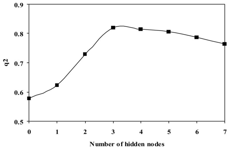
The dependence of q² on the number of hidden neurons of the 11-descriptor neural network model.

Figure 3.

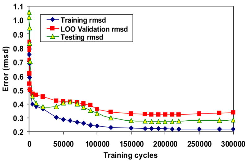
The training rmsd, LOO rmsd and testing as a function of the number of training cycles of NN11-3-1.

A common belief about neural network systems is that the number of parameters in the network should be related to the number of data points in the dataset, and the expressive power of the network.³⁹ For the current dataset, the results from the search for various configurations (Table 3) shows that the weights used in the neural network configuration to obtain better internal and external prediction are between 33 and 40. Comparing the NN11-3-1 model with the NN8-4-1 model, both configurations include 36 weights. While the numbers of descriptors used in both configurations are not overwhelmed (i.e., the ratio of the number of compounds in the training set to the number of descriptors is 8 and 11, respectively for NN11-3-1 and NN8-4-1), the former model includes more information from compounds themselves (i.e., a greater number of descriptors was used), and provides higher internal and external prediction ability (Table 3). Therefore, the best ANN model is an 11-descriptor model with 3 hidden neurons consisting of the following descriptors: Ram, PW5, LP1, SEige, VEp2, DISPm, G(N..N), H7m, RARS, R1p+, HOMT with 3 hidden nodes. Brief summaries of these descriptors can be found in Table 2.

3.2 Computational results

PLS analysis

The best PLS model for calculated descriptors is a 5-component model of 12 descriptors (Ram, PW5, DISPm, G(N..N), RCON, DISPp, HATS5u, R5u, R4u+, R1v+, R5v+, R5e+). The r² values for the training and for the LOO cross-validation runs are 0.83 and 0.78, respectively; the corresponding rmsd values are 0.303 and 0.353, respectively. For the 15 test compounds, the r² value is 0.87 and the rmsd is 0.415 (Table 4). Figure 4 shows the relationships of the trained, LOO and external predicted log(1/K_i) values versus the experimental log(1/K_i) values for the PLS model. The calculated log(1/K_i) values by the PLS model for the 104 molecules are shown in Table 1.

Table 4.

Statistical results for the best neural network model NN11-3-1 and the PLS model

Model	r2	rmsd	q2	loormsd
NN11-3-1
TSET	0.91	0.225	0.82	0.316
PSET	0.93	0.282
PLS
TSET	0.83	0.303	0.78	0.353
PSET	0.87	0.415

Figure 4.

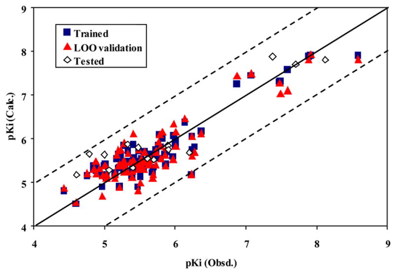
The calculated versus experimental activity data for the training (shown in squares), LOO cross-validation (shown in triangles) and test set runs (shown in diamonds) for the PLS QSAR model with VMAT2 ligands. The solid line represents a perfect correlation.

ANN analysis

The best 11-descriptor neural network model consists of the following descriptors: Ram, PW5, LP1, SEige, VEp2, DISPm, G(N..N), H7m, RARS, R1p+, HOMT. The statistical results for this model are as follows: r² =0.91, rmsd =0.225, q² = 0.82, and loormsd = 0.316. The QSAR model demonstrated good predictivity in the test set: r² =0.93, and rmsd = 0.282 (Table 4). Comparing the values of correlation coefficients and root mean square deviations listed in Table 4, the ANN model is better than the PLS model. The predictive ability of NN11-3-1 can also be judged from the plots of the trained, LOO and external test predicted versus experimental log(1/K_i) values shown in Figure 5. The computed log(1/K_i) values of the model for the 104 molecules in the database are listed in Table 1.

Figure 5.

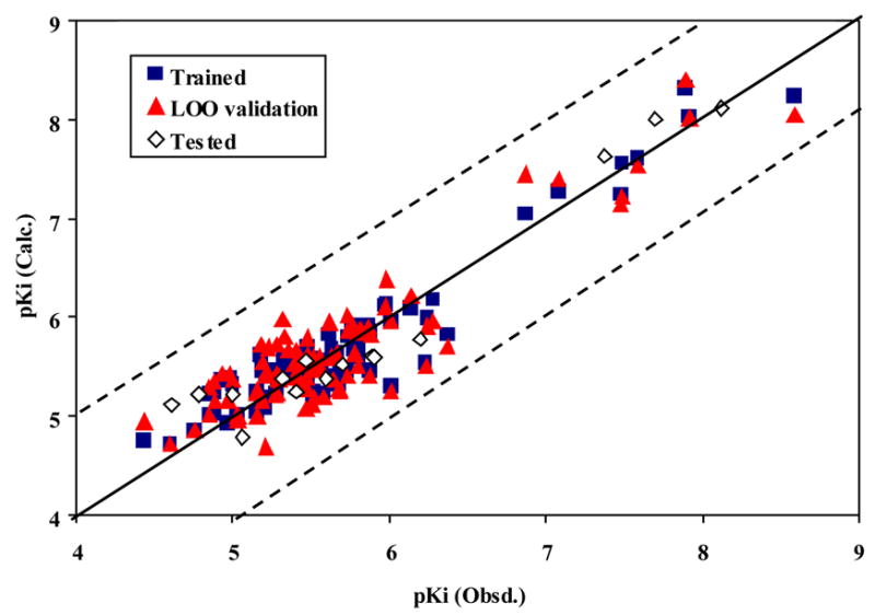
The calculated versus experimental activity data for the training (shown in squares), LOO cross-validation (shown in triangles) and test set runs (shown in diamonds) for the best NN11-3-1 QSAR model with VMAT2 ligands. The solid line represents a perfect correlation.

Descriptor contribution analysis

The statistics of the PLS model are summarized in Table 5. The X weights obtained from the PLS analysis are displayed in Table 6; the definition of the descriptors used in the model can be found in Table 2. Since q² beyond the 5^th component basically remains a constant for the PLS model, the most important descriptors may be located from the first 4 components only. In component 1, it is clear that PW5 and R5v+ are the most heavily weighted descriptors. PW5 is topological descriptors related to molecular shape;^35h R5v+ is one of the GETAWAY descriptors. According to the definition, GETAWAY descriptors are a type of descriptor encoding both geometrical information given by the influence molecular matrix and the topological information given by the molecular graph, weighted by chemical information encoded in selected atomic weightings.^35f GETAWAY descriptors are related to a molecular 3D structure. In the 2^nd component, the most weighted descriptors are two 3D descriptors - RCON and G(N..N), among which G(N..N) is a 3D geometrical descriptor and characterizes the geometrical distance between nitrogen and nitrogen in those molecules that contain more than one N-atom; RCON is referred to R-connectivity index, which is sensitive to the molecular size, conformational changes and cyclicity.^35f Accordingly, other relatively important descriptors identified by the component analysis were HATS5u, DISPp, R5e+ and DISPm. HATS5u and R5e+ are GETAWAY descriptors; DISPp and DISPm are geometrical descriptors. The details of these descriptors can be found in the previously published study.^35(b)–(h)

Table 5.

Summary of the PLS analysis for the 89 molecule training set^a

Component	r2	rmsd	F	q2	loormsd
1	0.662	0.420	170.0	0.615	0.448
2	0.772	0.347	145.8	0.681	0.409
3	0.817	0.312	126.8	0.750	0.365
4	0.825	0.307	99.3	0.762	0.358
5	0.832	0.303	81.9	0.780	0.353
6	0.835	0.302	69.2	0.771	0.356
7	0.837	0.302	59.3	0.772	0.357
8	0.838	0.303	51.6	0.774	0.357
9	0.838	0.305	45.3	0.772	0.361
10	0.838	0.307	40.3	0.772	0.364
11	0.838	0.309	36.1	0.772	0.366
12	0.838	0.311	32.7	0.772	0.369

^ar²: Pearson correlation coefficient, rmsd: root mean square deviation, F: Fishers estimate of statistical significance, q²: defined by Eq. (2), loormsd: LOO root mean square deviation.

Table 6.

X-Weights for the PLS components from the PLS analysis summarized in Table 5

No.*	Descriptor
	Ram	PW5	DISPm	G(N.N)	RCON	DISPp
1	0.374	0.460	0.310	0.060	0.275	−0.002
2	−0.245	0.229	0.378	−0.411	−0.541	−0.059
3	−0.356	−0.009	−0.264	−0.032	−0.328	−0.455
4	−0.431	−0.083	0.166	0.572	0.106	0.012
5	−0.268	−0.355	0.455	−0.379	0.128	0.330
6	0.045	−0.186	−0.192	−0.218	0.183	−0.457
7	−0.076	0.175	−0.051	0.242	−0.329	0.136
8	0.205	0.323	−0.391	−0.173	−0.245	0.245
9	0.398	−0.182	0.262	0.237	−0.466	0.110
10	−0.184	−0.086	−0.430	−0.166	0.064	0.593
11	0.208	−0.509	−0.105	0.239	−0.271	0.085
12	0.360	−0.366	−0.001	−0.279	−0.006	−0.149
No.*	Descriptor
	HATS5u	R5u	R4u+	R1v+	R5v+	R5e+
1	0.092	0.373	−0.136	−0.339	0.437	0.033
2	−0.166	−0.128	−0.209	0.041	0.236	−0.367
3	0.460	0.363	0.098	−0.308	0.082	0.181
4	−0.249	0.354	0.143	−0.021	0.007	−0.482
5	−0.031	0.408	0.074	0.001	−0.093	0.380
6	−0.637	0.147	−0.348	−0.274	−0.108	0.038
7	−0.498	−0.145	0.379	−0.172	0.267	0.512
8	−0.176	0.582	0.086	0.338	−0.222	−0.100
9	0.044	0.050	−0.098	−0.441	−0.493	−0.054
10	0.033	−0.086	−0.139	−0.530	0.168	−0.233
11	0.023	0.167	−0.400	0.292	0.519	0.079
12	−0.044	0.036	0.664	−0.096	0.255	−0.342

^*Component number.

The descriptors important for the NN11-3-1 model are plotted in Figure 6 according to a previous described procedure.^{24c, 40} The three most important descriptors are H7m, G(N..N) and DISPm. These descriptors indicate that molecular size, shape and atomic distribution in the molecules are important. The most important descriptor is the GETAWAY descriptor H7m. The second most significant descriptor, G(N..N), which is also an important descriptor in the PLS model. DISPm is related to the molecular geometry as well as molecular size; the other two important topological descriptors, PW5 and VEp2, also emphasize these important features. Among these important descriptors, PW5, G(N..N), and DISPm are common to both the PLS and the NN11-3-1 models. Analysis of the relationship between the values of the descriptors and the experimental endpoints of the compounds, several features were observed. To obtain an VMAT2 binding affinity K_i < 0.1 μM, it is shown that PW5 needs to be 0.12; H7m needs to be > 0.05 (most are between 0.05 and 0.15); VEp2 needs to be between 0.18 and 0.20; DISPm needs to be between 7.5 and 10.85; G(N..N) needs to be 0 or 4.34; and R1p+ needs to be between 0.03 and 0.05.

Figure 6.

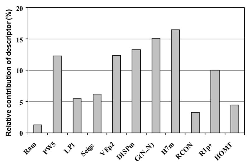
Relative contribution of descriptor plot for the NN11-3-1 neural network model built using the 89 VMAT2 ligands.

The linear PLS model and the NN11-3-1 model have five descriptors in common (Ram, PW5, DISPm, G(N..N), RCON). These descriptors are expected to significantly encode the linear relationship between the variables and the target bioactivity values. The neural network model contains five topological (Ram, PW5, LP1, SEige, VEp2) and six 3D descriptors (DISPm, G(N..N), H7m, RCON, R1p+, HOMT). These descriptors contain chemical information concerning size, symmetry, shape and distribution of the molecular atoms in the molecule. When compared to the linear model, the data show that the neural network model has been able to capture a more detailed analysis of the structure-activity relationships, and affords a high correlation with low root-mean-square-deviation.

Model stability analysis

To test the stability of the best neural network and PLS model, the dataset of 104 molecules was randomly divided into two sets; one set of 89 molecules for training and LOO validation, and the other set of 15 molecules for external testing. This process was randomly repeated five times. Among each division, the dissimilarity of one test set from the test set of another division was greater than 90%, i.e., less than one compound in 15 in one test set was the same as the compounds in another test set. The same eleven descriptors and the same neural network architecture, i.e., eleven input neurons, three hidden neurons and one output neuron, were used to train and test the neural network models. Learning epochs was set to 200,000. For the PLS model, the same twelve descriptors listed in Table 2 were used. Interestingly, during the five times training with the different set of eighty-nine molecules to build the PLS models, it was observed that the best PLS models are always those utilizing only five components of the twelve descriptors models for the five sets of data. The calculated results were listed in Table 7.

Table 7.

Stability analysis of the predictive models built from the set of 104 tetrabenazine and lobeline analogs

	NN11-3-1 model
No.	Train r2 (rmsd)	LOO q2 (rmsd)	Test r2 (rmsd)
1	0.91 (0.225)	0.82 (0.316)	0.93 (0.282)
2	0.93 (0.207)	0.83 (0.330)	0.89 (0.341)
3	0.93 (0.220)	0.81 (0.358)	0.92 (0.303)
4	0.92 (0.235)	0.84 (0.339)	0.88 (0.353)
5	0.93 (0.223)	0.80 (0.370)	0.94 (0.246)
Avg.	0.92 (0.222)	0.82 (0.343)	0.91 (0.305)
	PLS model
No.	Train r2 (rmsd)	LOO q2 (rmsd)	Test r2 (rmsd)
1	0.83 (0.303)	0.78 (0.352)	0.87 (0.415)
2	0.84 (0.319)	0.79 (0.373)	0.86 (0.380)
3	0.83 (0.330)	0.78 (0.388)	0.91 (0.301)
4	0.85 (0.338)	0.80 (0.379)	0.86 (0.330)
5	0.85 (0.320)	0.80 (0.373)	0.83 (0.403)
Avg.	0.84 (0.322)	0.79 (0.373)	0.87 (0.366)

The data in Table 7 indicate that the generated models are stable with regard to the data division. The neural network model has a higher predictive power than the PLS model. These results are consistent with the conclusions drawn previously (see section on descriptor contribution analysis).

4. Conclusion

In this study, PLS and neural network approaches were used to build linear and nonlinear QSAR models for a set of tetrabenazine and lobeline analogs that are ligands at the VMAT2. These are the first models to predict K_i values for the interaction of these two families of compounds with VMAT2. While the linear PLS model is predictive, it was demonstrated that the fully interconnected three-layer neural network model trained with the back-propagation procedure was to be superior in learning the correct association between a set of relevant descriptors of compounds and these log(1/K_i) for VMAT2. The trained neural network model (NN11-3-1) including eleven-input and three-hidden neurons exhibited a high predictive power (r²=0.91, rmsd=0.225 and q²=0.82, loormsd=0.316). This model succeeded in predicting the K_i values of an additional set of 15 tetrabenazine and lobeline analogs which were not included in the model training (external r²=0.93, rmsd=0.282). The stability test of the model with regard to data division was found to be positive. Evaluation of the contributions of the descriptors to the QSAR reflected the importance of atomic distribution in the molecules, molecular size and steric effects of the ligand molecules, when interacting with their target binding site on the VMAT2. The nonlinear relationship between these factors and the endpoint bioactivity values has been clearly demonstrated. These results indicate that the generated neural network model is reliable and predictive. Thus, this new neural network model, reported herein, will be valuable for future rational design of novel second generation ligands targeted to VMAT2, aimed at developing novel therapeutics for the treatment of methamphetamine abuse.

References and Notes

- 1.United Nations Office on Drugs and Crimes (UNODC) 2004 World Drug Report. http://www.unodc.org.
- 2.Nordahl TE, Salo R, Leamon MJ. Neuropsych Clin Neurosci. 2003;15:317. doi: 10.1176/jnp.15.3.317. [DOI] [PubMed] [Google Scholar]
- 3.Grace AA. Addiction. 2000;95:S119. doi: 10.1080/09652140050111690. [DOI] [PubMed] [Google Scholar]
- 4.Di Chiara G. Behav Brain Res. 2002;137:75. doi: 10.1016/s0166-4328(02)00286-3. [DOI] [PubMed] [Google Scholar]
- 5.Wise RA. Neuron. 2002;36:229. doi: 10.1016/s0896-6273(02)00965-0. [DOI] [PubMed] [Google Scholar]
- 6.Pifl C, Drobny H, Hornykiewicz O, Singer EA. Mol Pharmacol. 1995;47:368. [PubMed] [Google Scholar]
- 7.Sulzer D, Chen TK, Lau Y, Kristensen H, Rayport S, Ewing A. J Neurosci. 1995;15:4102. doi: 10.1523/JNEUROSCI.15-05-04102.1995. [DOI] [PMC free article] [PubMed] [Google Scholar]
- 8.Mantle TH, Tipton KF, Garrett NJ. Biochem Pharmacol. 1976;25:2073. doi: 10.1016/0006-2952(76)90432-9. [DOI] [PubMed] [Google Scholar]
- 9.Zheng G, Dwoskin LP, Deaciuc AG, Crooks PA. Bioorg Med Chem Lett. 2005;15:4463. doi: 10.1016/j.bmcl.2005.07.032. [DOI] [PMC free article] [PubMed] [Google Scholar]
- 10.Dwoskin LP, Crooks PA. Biochem Pharmacol. 2002;63(2):89–98. doi: 10.1016/s0006-2952(01)00899-1. [DOI] [PubMed] [Google Scholar]
- 11.(a) Eyerman DJ, Yamamoto BK. J Pharmacol Exp Ther. 2005;312:160. doi: 10.1124/jpet.104.072264. [DOI] [PubMed] [Google Scholar]; (b) Wilhelm CJ, Johnson RA, Lysko PG, Eshleman AJ, Janowsky A. J Pharmacol Exp Ther. 2004;310(3):1142. doi: 10.1124/jpet.104.067314. [DOI] [PubMed] [Google Scholar]
- 12.Teng L, Crooks PA, Crooks, Dwoskin LP. J Neurochem. 1998;71:258. doi: 10.1046/j.1471-4159.1998.71010258.x. [DOI] [PubMed] [Google Scholar]
- 13.Green TA, Miller DK, Wong WY, Harrod SB, Crooks PA, Bardo MT, Dwoskin LP. Soc Neurosci Abstr. 2001;878:1. [Google Scholar]
- 14.Miller DK, Crooks PA, Teng L, Witkin JM, Munzar P, Goldberg SR, Acri JB, Dwoskin LP. J Pharmacol Exp Ther. 2001;296:1023. [PubMed] [Google Scholar]
- 15.Harrod SB, Dwoskin LP, Green TA, Gehrke BJ, Bardo MT. Psychopharmacology. 2003;165:197. doi: 10.1007/s00213-002-1289-6. [DOI] [PubMed] [Google Scholar]
- 16.Perera RP, Wimalasna DS, Wimalasena K. J Med Chem. 2003;46:2599. doi: 10.1021/jm030004p. [DOI] [PubMed] [Google Scholar]
- 17.Lee LC, Borght TV, Sherman PS, Frey KA, Kilbourn MR. J Med Chem. 1996;39:191. doi: 10.1021/jm950117b. [DOI] [PubMed] [Google Scholar]
- 18.Canney DJ, Kung MP, Kung HF. Nucl Med Biol. 1995;22(4):521. doi: 10.1016/0969-8051(94)00118-4. [DOI] [PubMed] [Google Scholar]
- 19.Bruneau M-A, Lesperance P, Chouinard S. Letters to the Editor. Can J Psychiatry. 2002;47 doi: 10.1177/070674370204700716. [DOI] [PubMed] [Google Scholar]
- 20.Kenney C, Jankovic J. Expert Rev Neurotherapeutics. 2006;6:1. doi: 10.1586/14737175.6.1.7. [DOI] [PubMed] [Google Scholar]
- 21.Zheng G, Dwoskin LP, Deaciuc AG, Norrholm SD, Crooks PA. J Med Chem. 2005;48:5551. doi: 10.1021/jm0501228. [DOI] [PMC free article] [PubMed] [Google Scholar]
- 22.Zheng G, Dwoskin LP, Deaciuc AG, Norholm SD, Jones MD, Crooks PA. Bioorg Med Chem. 2005;13:3899. doi: 10.1016/j.bmc.2005.04.013. [DOI] [PMC free article] [PubMed] [Google Scholar]
- 23.Zheng G, Horton D, Deaciuc AG, Dwoskin LP, Crooks PA. Bioorg Med Chem. 2006 doi: 10.1016/j.bmcl.2006.07.070. in press. [DOI] [PMC free article] [PubMed] [Google Scholar]
- 24.(a) Ochoa C, Chana A, Stud M. Curr Med Chem Central Nervous System Agents. 2001;1:247. [Google Scholar]; (b) Kaiser KLE. Quant Struct-Act Relat. 2003;22:1. [Google Scholar]; (c) Zheng F, Bayram E, Sumithran SP, Ayers JT, Zhan CG, Schmitt JD, Dwoskin LP, Crooks PA. Bioorg & Med Chem. 2006;14(9):3017. doi: 10.1016/j.bmc.2005.12.036. [DOI] [PubMed] [Google Scholar]; (d) Katritzky AR, Pacureanu LM, Dobchev DA, Fara DC, Duchowicz PR, Karelson M. Bioorg & Med Chem. 2006;14(14):4987. doi: 10.1016/j.bmc.2006.03.009. [DOI] [PubMed] [Google Scholar]
- 25.Shah DR, Dev VR, Brown CA. M D computing: computers in medical practice. 1999;16(2):65. [PubMed] [Google Scholar]
- 26.Seker H, Odetayo MO, Petrovic D, Naguib RNG, Bartoli C, Alasio L, Lakshmi MS, Sherbet GV. Anticancer Res. 2002;22(1A):433. [PubMed] [Google Scholar]
- 27.Saidari S, Sardari D. Curr Pharm Des. 2002;8(12):659. doi: 10.2174/1381612024607199. [DOI] [PubMed] [Google Scholar]
- 28.Huuskonen J, Salo M, Taskinen J. Journal of Pharmaceutical Sciences. 2001;86(4):450. doi: 10.1021/js960358m. [DOI] [PubMed] [Google Scholar]
- 29.Li H, Yap CW, Xue Y, Li ZR, Ung CY, Han LY, Chen YZ. Drug Development Research. 2005;66(4):245–259. [Google Scholar]
- 30.Mager DE, Shirey JD, Cox D, Fitzgerald DJ, Abernethy DR. Journal of Pharmaceutical Sciences. 2005;94(11):2475. doi: 10.1002/jps.20384. [DOI] [PubMed] [Google Scholar]
- 31.Tripos discovery software package with SYBYL 6.8.1, (a) Tripos Inc., 1699 South Hanley Rd., St. Louis, Missouri, 63144, USA. Frisch MJ, Trucks GW, Schlegel HB, Scuseria GE, Robb MA, Cheeseman JR, Montgomery JA, Jr, Vreven T, Kudin KN, Burant JC, Millam JM, Iyengar SS, Tomasi J, Barone V, Mennucci B, Cossi M, Scalmani G, Rega N, Petersson GA, Nakatsuji H, Hada M, Ehara M, Toyota K, Fukuda R, Hasegawa J, Ishida M, Nakajima T, Honda Y, Kitao O, Nakai H, Klene M, Li X, Knox JE, Hratchian HP, Cross JB, Adamo C, Jaramillo J, Gomperts R, Stratmann RE, Yazyev O, Austin AJ, Cammi R, Pomelli C, Ochterski JW, Ayala PY, Morokuma K, Voth GA, Salvador P, Dannenberg JJ, Zakrzewski VG, Dapprich S, Daniels AD, Strain MC, Farkas O, Malick DK, Rabuck AD, Raghavachari K, Foresman JB, Ortiz JV, Cui Q, Baboul AG, Clifford S, Cioslowski J, Stefanov BB, Liu G, Liashenko A, Piskorz P, Komaromi I, Martin RL, Fox DJ, Keith T, Al-Laham MA, Peng CY, Nanayakkara A, Challacombe M, Gill PMW, Johnson B, Chen W, Wong MW, Gonzalez C, Pople JA. Gaussian 03. Gaussian, Inc; Pittsburgh, PA: 2003. Revision A.1.
- 32.Sulzer D, Sonders MS, Poulsen NW, Galli A. Progress in Neurobiology. 2005;75:406. doi: 10.1016/j.pneurobio.2005.04.003. [DOI] [PubMed] [Google Scholar]
- 33.(a) Huang XQ, Zheng F, Crooks PA, Dwoskin LP, Zhan CG. J Am Chem Soc. 2005;127:14401. doi: 10.1021/ja052681+. [DOI] [PMC free article] [PubMed] [Google Scholar]; (b) Huang XQ, Zheng F, Chen X, Crooks PA, Dwoskin LP, Zhan CG. J Med Chem. 2006;49(26):7661. doi: 10.1021/jm0606701. [DOI] [PubMed] [Google Scholar]
- 34.(a) Kilbourn MR, Lee LC, Heeg MJ, Jewett DM. Chirality. 1997;9:59. doi: 10.1002/(SICI)1520-636X(1997)9:1<59::AID-CHIR11>3.0.CO;2-P. [DOI] [PubMed] [Google Scholar]; (b) Kilbourn M, Lee L, Borght TV, Jewett D, Frey K. Eur J Pharmacol. 1995;278:249. doi: 10.1016/0014-2999(95)00162-e. [DOI] [PubMed] [Google Scholar]
- 35.(a) DRAGON software version 3.0, 2003, developed by Milano Chemometrics and QSAR Research Group (http://www.disat.nimib.it/chm/Dragon.htm); Todeschini R, Consonni V. Handbook of Molecular Descriptors. Wiley-VCH; Weinheim (Germany): 2000. Karelson M. Molecular Descriptors in QSAR/QSPR. Wiley-Interscience; new York (NY): 2000. Balaban AT, editor. From Chemical Topology to 3D Molecular Geometry. Plenum Press; New York (NY): 1997. Kubinyi H, Folkers G, Martin YC, editors. 3D QSAR in Drug Design. 1, 2, 3. Kluwer/ESCOM; 1996–98. Consonni V, Todeschini R, Pavan M. J Chem Inf Comput Sci. 2002;42:682. doi: 10.1021/ci015504a.Consonni V, Todeschini R. In: Rational Approaches to Drug Design. Hottje H-D, Sippl W, editors. Prous Science; Barcelona (Spain): 2001. pp. 235–240.Randic M. Acta Chim Slov. 1998;45:239.
- 36.Geladi P, Kowalski B. Analytica Chimica Acta. 1986;185:1. [Google Scholar]
- 37.Revised based on a C program originally from the neural network Senior Research Scientist Lars J. Kangas at Pacific Northwest National Laboratory
- 38.David MS. Building Neural networks. Addison; Wesley: 1996. p. 87. [Google Scholar]
- 39.Lawrence S, Giles CL, Tsoi AC. Lessons in neural network training: overfitting may be harder than expected; Proceedings of the Fourteenth National Conference on Artifical Intelligence, AAAI-97; AAAI Press, Menlo Park, California. 1997. pp. 540–545. [Google Scholar]
- 40.(a) Guha R, Jurs PC. J Chem Inf Model. 2005;45:800. doi: 10.1021/ci050022a. [DOI] [PubMed] [Google Scholar]; (b) Cherqaoui D, Villemin D. J Chem Soc, Faraday Trans. 1994;90:97. [Google Scholar]