

Abstract
Reference tissue model (RTM) is a compartmental modeling approach that uses reference tissue time activity curve (TAC) as input for quantification of ligand-receptor dynamic PET without blood sampling. There are limitations in applying the RTM for kinetic analysis of PET studies using [11C]Pittsburgh compound B ([11C]PIB). For region of interest (ROI) based kinetic modeling, the low specific binding of [11C]PIB in a target ROI can result in a high linear relationship between the output and input. This condition may result in amplification of errors in estimates using RTM. For pixel-wise quantification, due to the high noise level of pixel kinetics, the parametric images generated by RTM with conventional linear or nonlinear regression may be too noisy for use in clinical studies.
Methods
We applied RTM with parameter coupling and a simultaneous fitting method as a spatial constraint for ROI kinetic analysis. Three RTMs with parameter coupling were derived from a classical compartment model with plasma input: a RTM of 4 parameters (R1, k′2R, k4, BP) (RTM4P); a RTM of 5 parameters (R1, k2R, NS, k6, BP) (RTM5P); and a simplified RTM (SRTM) of 3 parameters (R1, k′2R, BP) (RTM3P). The parameter sets [k′2R, k4], [k2R, NS, k6], and k′2R are coupled among ROIs for RTM4P, RTM5P, and RTM3P, respectively. A linear regression with spatial constraint (LRSC) algorithm was applied to the SRTM for parametric imaging. Logan plots were used to estimate the distribution volume ratio (DVR) (= 1 + BP (binding potential)) in ROI and pixel levels. Ninety-minute [11C]PIB dynamic PET was performed in 28 controls and 6 individuals with mild cognitive impairment (MCI) on a GE Advance scanner. ROIs of cerebellum (reference tissue) and 15 other regions were defined on coregistered MRI’s.
Results
The coefficients of variation of DVR estimates from RTM3P obtained by the simultaneous fitting method were lower by 77 - 89% (in striatum, frontal, occipital, parietal, and cingulate cortex) as compared to that by conventional single ROI TAC fitting method. There were no significant differences in both TAC fitting and DVR estimates between the RTM3P and the RTM4P or RTM5P. The DVR in striatum, lateral temporal, frontal and cingulate cortex for MCI group was 25% to 38% higher compared to the control group (p ≤ 0.05), even in this group of individuals with generally low PIB retention. The DVR images generated by the SRTM with LRSC algorithm had high linear correlations with those from the Logan plot (R2 = 0.99). In conclusion, the RTM3P with simultaneous fitting method is shown to be a robust compartmental modeling approach that may be useful in [11C]PIB PET studies to detect early markers of Alzheimer’s disease where specific ROIs have been hypothesized. In addition, the SRTM with LRSC algorithm may be useful in generating R1 and DVR images for pixel-wise quantification of [11C]PIB dynamic PET.
Introduction
Positron emission tomography (PET) with [11C]Pittsburgh compound B ([11C]PIB) has been used for in vivo imaging of amyloid-β (Aβ) in Alzheimer’s disease (AD), mild cognitive impairment (MCI), and aging in humans (Mathis et al., 2004; Buckner et al., 2005; Klunk et al., 2004, 2005). The full chemical name for [11C]PIB is [N-methyl-11C]2-(4′-methylaminophenyl)-6-hydroxybenzothiazole (or [11C]6-OH-BTA-1) that has binding affinity KD = 1.4 nM for homogenates of post-mortem AD frontal cortex and KD = 4.7 nM for synthetic Aβ (Mathis et al., 2003). Human studies using [11C]PIB PET have indicated greater retention of [11C]PIB in the brains of AD patients and subjects with MCI as compared to the healthy controls (Price et al., 2005; Lopresti et al., 2005; Mintun et al., 2006), as well as an inverse association between PIB retention and CSF Aβ (Fagan et al., 2006). [11C]PIB is the most widely used PET imaging agent (the other is [18F]FDDNP) in research studies aimed at improving early detection of AD, monitoring progression of Aβ deposition in the brain, and evaluating anti-amyloid and other therapies to stop progression of AD (Shoghi-Jadid et al., 2002; Mathis et al., 2004; Mintun 2005; Nichols et al., 2006; Nordberg 2004; Small et al., 2006; Wu et al., 2005).
The standard compartmental model with plasma input as well as model-independent spectral analysis and graphical analysis (Logan plot) with plasma input were used for [11C]PIB kinetic analysis (Price at al., 2005; Verhoeff et al., 2004). Consistent results from the two previous studies demonstrated that 1) a 2-tissue compartmental model provided better cure fitting than 1-tissue compartmental model; 2) the Logan plot with plasma input is a robust approach to estimate [11C]PIB distribution volume (DV) as compared to the 2-tissue compartmental model; and 3) there was no significant difference in the DV estimates for reference tissue (cerebellum) between controls and AD patients. The plasma input is usually obtained by arterial blood sampling during the PET study period, and tracer metabolism in plasma is corrected using the HPLC technique. This procedure is laborious and is associated with experimental errors and risks to subjects, particularly in the context of frequent longitudinal follow-up. Thus, the ability to conduct accurate studies without arterial sampling will increase the feasibility of [11C]PIB for clinical practice and increase recruitment and retention of participants within the context of large, longitudinal studies. To quantify [11C]PIB dynamic PET without arterial blood sampling, compartmental model with the plasma input derived from dynamic image data, graphical analysis (Logan plot) and a simplified reference tissue model (SRTM) with reference tissue input, and standardized uptake value ratio (SUVR) or target to reference tissue concentration ratio were evaluated (Edison et al., 2007; Fagan et al., 2006; Kemppainen et al., 2006; Lopresti et al., 2005; Price et al., 2005).
Reference tissue model is a compartmental modeling approach that uses the reference tissue time activity curve (TAC) as input (Cunningham et al., 1991; Gunn et al., 2000; Lammertsma et al., 1996; Lammertsma and Hume 1996; Morris et al., 2005; Watabe et al., 2000). In contrast to graphical analysis, the parameters of reference tissue model are estimated by fitting the model to the full time course of tissue TAC measured by PET. Analogous to the classical compartmental model with plasma input, the reference tissue model can be used to predict and simulate tissue tracer kinetics with given model parameters and reference tissue input. Compared to graphical analysis, the reference tissue model is commonly used to extract more physiological information from measured tracer kinetics, such as the relative tracer transport rate constant from vascular space to tissue. In addition, reference tissue models have been extended for kinetic analysis of dynamic PET with pharmacological challenges or cognitive activation during PET (Alpert et al., 2003; Votaw et al., 2002; Watabe et al., 1998; Zhou et al., 2006a).
On the other hand, in theory, there is a limitation in using reference tissue models for the tissue tracer kinetics of low or even negligible specific binding. This is because the low and negligible specific binding of [11C]PIB in target tissue can result in a high linear relationship between the output and input for the reference tissue model. This situation may amplify the errors noticeably in estimates obtained through the reference tissue model. For example, a convergence problem in nonlinear fitting of SRTM to [11C]doxepin ROI TAC occurred in tissues of low H1 receptor BP (Suzuki et al., 2005). It was also reported that the estimates of low BP obtained by conventional nonlinear SRTM fitting were not reliable in [11C]PIB and [11C]SB-13 PET studies (Verhoeff et al., 2004; Zhou et al., 2006b). Previous [11C]PIB studies have reported that BP was close to 0, or the distribution volume ratio DVR (= 1+BP) was close to 1, in most cortical regions in controls. Estimates of PIB retention were also low in brain regions with negligible Aβ load in MCI and AD patients (Lopresti et al., 2005; Price et al., 2005). It has been demonstrated that the accuracy of estimates can be improved by simultaneously fitting a compartmental model with plasma input or reference tissue input to multiple ROI TACs (Buck et al., 1995; Cunningham et al., 2004, Endres et al., 2003; Ginovart et al., 2001; Raylman et al., 1994; Zhou et al., 2006b). For this approach, the coupled parameter or parameters can be estimated simultaneously for all ROIs. In contrast, the coupled parameter estimated by fitting the model to each single ROI TAC, the conventional ROI TAC model fitting procedure, usually varies among ROIs and this is not consistent with model assumption.
The use of higher order reference tissue models, i.e., more compartments used for target and reference tissues, has been proposed to reduce the bias of BP or DVR estimates from the SRTM (Endres et al., 2003; Kropholler et al., 2006; Wu and Carson, 2002; Zhou et al., 2006c). In this study, three reference tissue models were used for ROI kinetic modeling and their estimates were compared to investigate if there are any significant improvements using higher order reference tissue models. To obtain reliable estimates of model parameters, reference tissue models with parameter coupling were derived and implemented by simultaneous fitting for ROI based quantification. As a comparison, a reference tissue model with the conventional single ROI TAC fitting method was also applied to same ROI data set.
The parametric images that represent both the spatial distribution and quantification of the physiological parameters are generated by fitting a tracer kinetic model to the measured individual pixel time activity curves. However, due to the inherent high noise level of pixel kinetics of PET, the parametric images generated by conventional linear or nonlinear fitting are usually less accurate than those obtained by model fitting with spatial-temporal analysis (Gunn et al., 2002; Kimura et al., 1999; Turkheimer et al., 2003; Zhou et al., 2002, 2003). In this study, a linear regression with spatial constraint algorithm (LRSC) we previously developed (Zhou et al., 2003) was applied to the SRTM model for pixel-wise quantification of [11C]PIB kinetics. The R1 and DVR images generated by the SRTM with the LRSC algorithm were compared to the estimates from ROI kinetic analysis and pixel-wise Logan plot. The [11C]PIB dynamic PET data for 28 controls and 6 individuals with MCI were used in the study.
Materials and Methods
Theory of reference tissue model with parameter coupling
The reference tissue model is derived from classical compartmental model theory by eliminating plasma input with reference tissue TAC. In clinical ligand-receptor PET studies, a 2-tissue compartmental model with plasma input (Fig. 1) is commonly used to fit the measured reversible tracer kinetics for both target and reference tissues (Huang, et al., 1986; Koeppe et al., 1991; Lammertsma et al., 1996; Mintun et al., 1984; Price et al., 2005). The tracer kinetics described by Fig. 1 are based on the following assumptions: 1) rapid equilibrium between free and nonspecific binding in target tissue is attained; 2) the concentrations of tracer are homogenous in vascular space (CP), free plus nonspecific binding compartment (CF+NS), and specific binding compartment (CS) for target tissue, free and nonspecific binding compartments (CF, and CF+NS) for reference tissue; and 3) the transport of tracer between compartments has first order kinetics. Based on above assumptions, the tracer kinetics in target and reference tissues are described by the following differential equations:
Fig.1.

A representative 2-tissue compartmental model used in ligand-receptor PET studies for target and reference tissues. The concentrations in vascular space (CP), free and nonspecific binding compartment (CF+NS), specific binding compartment (CS) for target tissue, and free and nonspecific binding compartments (CF, and CF+NS) for reference tissue are assumed to be homogeneous. The transport of tracer between compartments has first order kinetics with rate constants K1 to k6.
| (1) |
| (2) |
| (3) |
| (4) |
Reference tissue model assumes that the tissue tracer activity contributed from vascular space is negligible, i.e., CT = CF+NS + CS, and CR = CF + CNS, where the CT and CR are the tracer concentrations in target and reference tissues measured by the PET scanner, CF+NS(0) = CS(0) = CF(0) = CNS(0)=0, K1 (ml/min/ml) is the transport rate constant from vascular space to target tissue, k2 (1/min) is the efflux rate constant from free plus nonspecific compartment to blood, k3 (1/min) is the rate of specific receptor binding, and k4 (1/min) is rate of dissociation from receptors, K1R (ml/min/ml) is the transport rate constant from vascular space to reference tissue, k2R (1/min) is the efflux rate from free compartment in reference tissue to blood, k5 (1/min) is the rate constant of nonspecific receptor binding, and k6 (1/min) is rate of dissociation from nonspecific binding. One common measure of tracer binding kinetics is the distribution volume (DV). The tracer DV in tissue or compartment is defined as the ratio of the tracer concentration in tissue or compartment to the tracer concentration in plasma at equilibrium condition. The primary measure for quantification of ligand-receptor dynamic PET is BP that is defined as BP = f2B′max/KD, where f2 is the free fraction of tracer in the free and nonspecific binding compartment, B′max (nM) is the available receptor density for tracer binding, and KD (nM) is the tracer equilibrium dissociation constant. BP is an index of tracer specific binding to receptor (Huang et al., 1986; Mintun et al., 1984). In terms of model micro-parameters, BP in target tissue, DV in free plus nonspecific binding compartment (DVF+NS), in target tissue (DVT), and in reference tissue (DVREF) can be expressed as BP = k3/k4, DVF+NS = K1/k2, DVT = (K1/k2)(1+k3/k4), and DVREF = (K1R/k2R)(1+k5/k6). The essential assumption to derive the reference tissue model is that the tracer distribution of volume in free plus nonspecific binding compartment is identical between reference tissue and target tissue, i.e.: DVF+NS =DVREF. The estimation of micro-parameters can be affected by spatial heterogeneity of tracer kinetics, and so the estimated values may not be consistent with the assumed physiological meaning (Cunningham et al., 2004; Herholz et al., 1990; Zhou et al., 1997). Thus, the reliable and robust estimate for BP is often estimated as BP=DVT/(K1/k2) - 1 = DVT/DVREF - 1 = DVR - 1, DVR (= DVT/DVREF) is the distribution volume ratio between target and reference tissues.
The DVR or BP can be estimated directly by reference tissue models using the reference tissue TAC as input. The reference tissue model derived from a 2 compartments for both target and reference tissues (Fig. 1) has 7 parameters, and it usually results in model identity problems in clinical situations (Kropholler et al., 2006, Wu and Carson 2002). The following three reference tissue models with lower orders of model configuration described in Fig. 2 were rederived for models incorporating parameter coupling and were compared in the present study.
Fig. 2.

The compartmental model configurations used to derive three reference tissue models. A: Under the assumption that rapid equilibrium is attained between free and nonspecific binding in reference tissue, the tracer concentration in reference tissue (CR) is modeled with a single compartment. B: With the assumption of rapid equilibrium between free plus nonspecific binding and specific binding, the total concentration in target tissue CT is modeled by a single compartment; and C: Under the assumptions from A and B, the tracer concentration in target tissue (CT) and reference tissue (CR) can be modeled by a single compartment. CP is the tracer concentration in vascular space as input function. K1 to k6, K1R, k′2, k2R, and k′2R are the transport rate constants between compartments.
Full reference tissue model with parameter coupling-RTM4P
A conventionally employed full reference tissue model with 4 parameters (R1, k2, k3, k4) is shown in Fig. 2 A (Lammertsma et al., 1996). Under the assumption that rapid equilibrium is attained between free and nonspecific binding in reference tissue, the tracer concentration in reference tissue (CR) is modeled with a single compartment. The reference tissue model with four parameters (R1, k′2R, k3, k4) (RTM4P) is then derived from 2 compartments for target tissue and 1 compartment for the reference tissue as below.
The tracer kinetics in target and reference tissue described by Fig. 2 A follow Eqs. (1)-(2) and Eq. (5) as below.
| (5) |
where k′2R (1/min) is the efflux rate from reference tissue to blood. Based on the assumption on DVF+NS, i.e., K1/k2 = K1R/k′2R. Let R1=K1/K1R, we have k2 = (K1/ K1R) k′2R = R1 k′2R, By applying a Laplace transform to Eqs (1)-(2) and Eq. (5) with initial conditions CF+NS(0) = CS(0) = CR(0) = 0, the operational equation for RTM4P can be expressed by parameters of R1, k′2R, k4 and BP:
| (6) |
where , , , k2 = R1 k′2R, k3 = BP k4, and ⊗ is the mathematical operation of convolution. The k′2R and k4 are the coupled parameters among all ROIs for RTM4P.
“Watabe” reference tissue model with parameter coupling-RTM5P
Symmetrically, the configuration for the second reference tissue model is usually referred to as the “Watabe” reference tissue model with parameters (R1, k′2, k2R, k5, k6) (see Fig. 2 B (Endres et al., 2003; Gunn et al., 2001; Kropholler et al., 2006; Millet et al., 2002; Watabe et al., 2000). With the assumption of rapid equilibrium between free plus nonspecific binding and specific binding, tracer concentration CT for target tissue can be modeled by a single compartment. Therefore, in addition to the Eq. (3)-(4) for tracer kinetics in reference tissue, the tracer kinetics in target tissue follows Eq. (7).
| (7) |
where k′2 is the transport rate constant from target tissue to blood. Note that k′2 = k2/(1 + BP), and k′2R = k2R/(1 + NS) (NS = k5/k6). The operational equation for RTM5P is then expressed by parameters of R1, k2R, NS, k6, and BP as below.
| (8) |
where k5=k6NS, , , and . For RTM5P, the parameters k2R, NS, k6 are coupled among all ROIs.
SRTM with parameter coupling-RTM3P
The last reference tissue model with configuration demonstrated by Fig. 2 C is commonly referred as the SRTM with parameters (R1, k2, and BP) (Lammertsma and Hume, 1996). The model with configuration Fig. 2 C assumes that the tracer concentrations in target and reference tissues can be modeled by a single compartment. The tracer kinetics in target and reference tissues for the SRTM are therefore determined by Eqs. (5) and (7). Based on DVF+NS = DVREF, we have k2 = (K1/ K1R) k′2R = R1 k′2R, and the SRTM with (R1, k′2R, BP) is referred to as RTM3P for consistency in this study. The operational equation for the RTM3P is then written as Eq. (3).
| (9) |
The k′2R implies only one parameter coupled among all ROIs for RTM3P.
Simultaneously fitting model to all ROI TACs
To embody the physiological assumptions into the model fitting process for the reference tissue model with parameter coupling, and to reduce the variability of estimates, simultaneously fitting a model to all ROI TACs has been used in ligand-receptor dynamic PET (Buck et al., 1995; Cunningham et al., 2004, Endres et al., 2003; Raylman et al., 1994; Zhou et al., 2006b, 2006c). For the above three reference tissue models with parameter coupling, the cost function to be minimized for RTM3P, RTM4P, and RTM5P are: , , and , respectively
Where M is the number of time frames for dynamic PET scans and N is number of ROI TACs, ti is the mid time of ith frame of dynamic PET scanning, wi is the duration of ith frame of dynamic PET scanning, Cj (ti) is the measured jth ROI’s tracer concentration at ith frame. The jth ROI’s tracer concentration at time ti are determined by fRTM 3P, fRTM 4P, and fRTM 5P with the parameters , BPj for jth ROI and the coupled parameters k′2R, (k′2R, k4) and (k2R, NS, k6) for RTM3P, RTM4P, and RTM5P, respectively. The Marquardt algorithm, a conventional nonlinear regression algorithm, was used to minimize cost function (Marquardt 1963).
For comparison, the parameters of the reference tissue models were also estimated by fitting RTM3P, RTM4P and RTM5P to each single ROI TAC. In contrast, the cost function for fitting model to individual jth ROI TAC is: , , and for RTM3P, RTM4P, and RTM5P, respectively.
To compare with previous results (Price et al., 2005; Lopresti et al., 2005), DVR was calculated as BP + 1 after model fitting. The Akaike information criterion (AIC) (Akaike 1976, Carson et al., 1993, Turkheimer et al., 2003) was calculated for simultaneous fitting. The AIC for the reference tissue model with conventional single ROI fitting method was calculated as .
Linear regression with spatial constraint for parametric imaging
Based on the results from ROI kinetic analysis (the estimates of R1, and DVR from RTM3P, RTM4P and RTM5P were almost same, see Comparison of reference tissue models subsection of Results section), the SRTM model was used to generate parametric images. To improve the accuracy of pixel-wise estimates, a linear regression with spatial constraint (LRSC) algorithm was applied to Eq. (10) and Eq. (11) to generate R1, and DVR images, respectively (Zhou et al., 2003).
| (10) |
| (11) |
To perform pixel-wise statistical analysis, all the parametric images were spatially normalized to the standard space (pixel size: 2×2 mm2, slice thickness 2 mm) using SPM2 (statistical parametric mapping software; Wellcome Department of Cognitive Neurology, London, UK). Because the R1 images contain greater structural information, the R1 images generated by LRSC were used to determine the parameters of spatial normalization. These transformation parameters were applied to all generated parametric images for each subject. Two iterations of the spatial normalization process were performed: 1) the parameters obtained by normalizing R1 images to the R1 template generated in our previous [11C]raclopride study (Zhou et al., 2003), and 2) mean R1 images obtained by first iteration were used as a template for the second iteration.
Logan plot with reference tissue input
The standard Logan plot with reference tissue input was used for estimation of the DVR of [11C]PIB binding in previous studies (Lopresti et al., 2005, Mintun et al., 2006). As compared to the standard Logan plot with reference tissue input, one advantage of the simplified Logan plot with reference tissue input is that it eliminates the need to estimate the mean of k′2R (Logan et al., 1996). The simplified Logan plot given by Eq. (12) was proposed for ROI based [11C]PIB kinetic analysis in this study.
| (12) |
To obtain robust DVR estimates for pixel TACs of high noise levels, the simplified Logan plot in bilinear form as below was used to generate DVR images.
| (13) |
where t* = 40 min.
For comparison, the standard Logan plot using Eq. (14) was also applied to the ROI TACs to estimate ROI DVR in the study.
| (14) |
where is a population average value of k′2R. The estimated by a 2-tisue compartment, 4-parameter model with plasma input was 0.08/min for controls (n = 5), 0.07/min for MCI (n = 5) and AD (n = 4) (Price et al., 2005). The was also fixed at 0.149/min and 0.2/min for Logan plot with reference tissue input in [11C]PIB PET studies by Lopresti and Mintun (2006), respectively. Note that the estimated by RTM3P for controls (n = 28) and MCIs (n = 6) was 0.05/min in our current study (see Results section). To investigate the effects of on the DVR estimates, we estimated DVR with a fixed series of values from 0.03/min to 0.5/min and compared these to the simplified Logan plot approach given by Eq. (12).
Human [11C]PIB imaging and data acquisition
Subjects were 34 of the first 36 participants (excluding one with a clinical stroke and one with missing PET time frames due to scanner error) evaluated with [11C]PIB as part of the ongoing neuroimaging substudy of the Baltimore Longitudinal Study of Aging (BLSA) (Resnick et al., 2000, 2003). At initial enrollment, BLSA neuroimaging participants were free of dementia and other central nervous system disorders, severe cardiovascular disease, and metastatic cancer (detailed in Resnick et al., 2000). [11C]PIB studies were initiated in June 2005, and participants had been followed for up to 12 years with structural and functional imaging studies. Evaluation of diagnostic status followed established BLSA procedures, using prospective follow-up information (detailed in Gamaldo et al 2006). All participants received a detailed physical examination, including medical history updates and laboratory screening, neuropsychological testing, and assessment by the Clinical Dementia Rating (CDR) (Morris et al., 2001) scale in conjunction with the [11C]PIB study. The CDR scores were typically based on informant interviews (spouse, child, or close friend) conducted by a certified examiner. Participant data was reviewed at a consensus diagnostic conference if the Blessed-Information-Memory-Concentration (BIMC; Blessed et al., 1968) test score was 3 or above or if the informant or subject CDR score was 0.5 or above. Diagnoses were made at consensus diagnostic conferences using DSM-III-R (APA, 1987) criteria for dementia and the NINCDS-ADRDA criteria (McKhann et al., 1984) using neuropsychological diagnostic tests and clinical data. A diagnosis of mild cognitive impairment not meeting criteria for dementia was made for participants who had cognitive impairment (typically memory) but did not have functional loss in activities of daily living. One participant in the present study met stringent diagnostic criteria for mild cognitive impairment and five additional participants scored 0.5 on the CDR scale, reflecting very mild cognitive impairment. Normal controls had scores of 0 on the CDR and were considered cognitively normal by our diagnostic procedures. It is important to emphasize that the MCI participants in this study are identified within the context of prospective longitudinal follow-ups and represent very mild cases of cognitive impairment in contrast to those followed in other studies who typically present with memory complaints.
Structural magnetic resonance imaging (MRI) scans and [11C]PIB dynamic PET were acquired for each participant. MRI and PET imaging are typically performed on the same visit, but a major renovation of the MRI research scanners coincided with the initial PIB imaging studies. MRI scans were acquired within 3 days of the PET scan for 16 participants and within 1 to 2 years for 15 participants. Excluding 3 individuals, where it was necessary to use an MRI obtained 4, 5, and 10.5 years prior, respectively, the mean (SD) interval between MRI and PET was 0.6 (0.8) years.
MRI scans for anatomic localization were performed on a 1.5 Tesla GE Signa system using a spoiled gradient recalled acquisition sequence (124 slices with image matrix 256×256, pixel size 0.93×0.93 mm, slice thickness 1.5 mm). Dynamic PET [11C]PIB studies were performed on a GE Advance scanner. The PET scanning was started immediately after intravenous bolus injection of 14.45 ± 1.01 (n = 34, range 11.02 to 16.36) (mean ± SD hereafter for “±”) mCi [11C]PIB with a specific activity of 4.29 ± 1.49 (n = 34, range 0.96 to 6.83) Ci/μmol. Dynamic scans were acquired in 3D mode with acquisition protocol of 4×0.25, 8×0.5, 9×1, 2×3, 14×5 min (total 90 min, 37 frames). To minimize motion during PET scanning, all participants are fitted with thermoplastic face masks for the PET imaging. Ten-minute 68Ge transmission scans acquired in 2-D mode were used for attenuation correction of the emission scans. Dynamic images were reconstructed using filtered back projection with a ramp filter (image size 128×128, pixel size 2×2 mm, slice thickness 4.25 mm), which resulted in a spatial resolution of about 4.5 mm FWHM at the center of the field of view. MRIs were coregistered to the mean of the first 20 min dynamic PET images using SPM2 with a mutual information method. In addition to the reference region (cerebellum), fifteen ROIs (1: caudate, 2: putamen, 3: thalamus, 4: lateral temporal, 5: mesial temporal, 6: orbital frontal, 7: prefrontal, 8: occipital, 9: superior frontal, 10: parietal, 11: anterior cingulate, 12: posterior cingulate, 13: pons, 14: midbrain, 15: white matter) were manually drawn on the coregistered MRIs (Price et al., 2005, Lopresti et al., 2005) and copied to the dynamic PET images to obtain ROI TACs for kinetic analysis. The ROIs estimates were also obtained by applying ROIs to parametric images.
Results
Control and mild cognitive impairment (MCI) group
There were 28 individuals (17 males, 11 females, age range 55-92 years, 78.6 ± 8.1) with CDR = 0 that were classified as the normal control group, and 6 individuals (2 males, 4 females, age range 77-89, 83.0 ± 4.2) in the MCI group. The difference in age between the control and MCI groups was not statistically significant.
Improvements in estimates by model fitting with parameter coupling
The variation in DVR from RTM3P estimates from conventional single ROI TAC fitting method (cost function determined by single ROI TAC) was reduced remarkably by the simultaneous fitting method in caudate, putamen, and most cortical regions in the control group. As demonstrated by Fig. 3, the coefficients of variation (CV), defined as 100mean/(standard deviation) of DVR estimates, from the conventional method were reduced from 77% to 89% in caudate, putamen, orbital frontal cortex, prefrontal cortex, occipital cortex, superior frontal cortex, parietal cortex, anterior cingulate cortex, and posterior cingulate cortex in control group. The DVR estimated by the simultaneous fitting method were comparable to those estimated by the conventional method for the ROIs of thalamus, lateral temporal, mesial temporal cortex, pons, midbrain, and white matter in control group. For the MCI group, an improvement in the DVR estimates for the simultaneous fitting method relative to the conventional method was only found in the occipital cortex.
Fig.3.

The coefficient of variation of DVR estimates (=100* (mean/(standard deviation))) for the control group (n = 28) and MCI group (n = 6). The DVR estimates were obtained from the RTM3P model with simultaneous fitting and single ROI TAC fitting methods. Regions of interest are numbered as: 1: caudate, 2: putamen, 3: thalamus, 4: lateral temporal, 5: mesial temporal, 6: orbital frontal, 7: prefrontal, 8: occipital, 9: superior frontal, 10: parietal, 11: anterior cingulate, 12: posterior cingulate, 13: pons, 14: midbrain, 15: white matter.
The mean plus standard deviation of k′2R of RTM3P is shown in Fig. 4. k′2R, the efflux rate constant from reference tissue to blood, is expected to be the same for all ROIs in the RTM3P model but shows high variation in estimates from the conventional single ROI TAC fitting method. The estimates of k′2R vary from 0.01 ± 0.02 for prefrontal cortex to 0.15 ± 0.05 for thalamus in the control group, and from 0.01 ± 0.01 for occipital cortex to 0.14 ± 0.05 for thalamus in the MCI group. If k′2R is estimated by the mean over all 15 ROIs, i.e., k′2R (mean) = , the k′2R(mean) is significantly lower than that estimated by the simultaneous fitting approach (paired t test, p < 0.01) for the control group. The k′2R (mean) in the control group tends to be lower than that in the MCI group (0.04 ± 0.01 versus 0.05 ± 0.01, p = 0.09), while the coupling method yields greater similarity between k′2R for the control and MCI groups (0.05 ± 0.01 versus 0.05 ± 0.01, p = 0.42). R1 estimates from the conventional and simultaneous fitting methods do not differ significantly (p = 0.77). It was also found that R1 estimates from the conventional fitting method were high linearly correlated with those from the simultaneous fitting method as R1(simultaneous fitting) = 0.96R1(conventional) + 0.03 (R2 = 0.95).
Fig. 4.

The mean plus standard deviation of k′2R estimates from the RTM3P model with simultaneous fitting and single ROI TAC fitting methods for the control group (n = 28) and MCI group (n = 6). k′2R is the efflux rate constant from reference tissue (cerebellum) to blood. The mean of k′2R estimates over 15 ROIs after single ROI TAC fitting is also shown. Regions of interest are numbered as: 1: caudate, 2: putamen, 3: thalamus, 4: lateral temporal, 5: mesial temporal, 6: orbital frontal, 7: prefrontal, 8: occipital, 9: superior frontal, 10: parietal, 11: anterior cingulate, 12: posterior cingulate, 13: pons, 14: midbrain, 15: white matter.
The reduction of variation for k′2R and DVR estimates in parametric space for the simultaneous fitting approach is at the cost of higher residual sum of squares in kinetic space (cost function values) or AIC as compared to the conventional single ROI fitting approach. For the RTM3P model, the AIC of model fitting with the simultaneous fitting approach is higher (6 ± 3)% than that from the conventional fitting method. Note that the better fit or lower AIC mostly occurs in ROIs of lower DVR (< 1.5). Representative TACs are shown for a control in Fig 5 panel A1 and A2 and an MCI individual in Fig. 5 panel B1 and B2. As demonstrated by Fig. 5, the fitted ROI TACs from the simultaneous fitting and single ROI TAC fitting methods were quite comparable visually for (6 ± 3)% difference in AIC. Fig. 5 also illustrates that, as DVR increases, for example in posterior cingulate cortex, from controls to MCI, the difference in the fitted curves between the simultaneous fitting approach and conventional method tends to be smaller.
Fig. 5.

Typical time activity curves (TACs) from the [11C]PIB dynamic PET studies from a control subject A (panel A1 and A2) and from a MCI subject B (panel B1 and B2). The fitted curves are from a reference tissue model RTM3P(R1, k′2R, BP) with a simultaneous ROI TAC fitting approach (A1 and B1) and a conventional single ROI TAC fitting method.
Comparison of reference tissue models
The results presented above suggest that estimates of the reference tissue model from the conventional single ROI TAC fitting method show high variability under conditions of low binding. Thus, in this section we base our comparison of parameter estimates from different reference tissue models on the simultaneous fitting approach. The AICs from SRTM3P, SRTM4P, and SRTM5P were -3184.39 ± 205.68, -3194.23 ± 195.01, and -3194.08 ± 201.67, respectively. Compared to RTM3P, there were no significant reductions in AIC by RTM4P (paired t test, p = 0.84) or RTM5P (paired t test, p = 0.85). Thus, there was no significant improvement in model fitting in kinetic space from RTM4P and RTM5P, as compared to RTM3P. Consistently, Fig. 6 shows that the estimates of R1, and DVR from RTM3P were almost identical to those estimated from RTM4P and RTM5P. The k′2R estimates from all three models were 0.05 ± 0.01 (n = 34), and there were no significant differences for k′2R among the three models (p = 0.52 for RTM3P versus RTM4P and p = 0.71 for RTM3P versus RTM5P). Note that the k′2R was calculated as k2R /(1+NS) after fitting for RTM5P. The coupled parameter k4 estimates of RTM4P were 0.56 ± 0.24, and 0.40 ± 0.22 for controls and MCI subjects, respectively, and not significantly different (p = 0.16). For RTM5P, the estimates of NS (= k5/k6) were 0.17 ± 0.30, and 0.13 ± 0.24 for control and MCI, respectively (p = 0.76, not significant). The estimates from RTM5P for the coupled parameter k6 were 0.80 ± 0.23 and 0.63 ± 0.45 for control and MCI, respectively (p = 0.40, not significant).
Fig. 6.

R1, k′2R, and DVR estimated by RTM3P versus those from RTM4P and RTM5P. The k′2R was calculated as k2R/(1+NS) after fitting for RTM5P. The simultaneous fitting method was used for RTM3P, RTM4P, and RTM5P (see text for reference tissue model definitions).
DVR estimates from Logan plots
The linear correlations between the DVR from Logan plot (simplified version) and the standard Logan plot with pre-determined were:
,
,
, and
.
Thus, the DVR estimates from the Logan plot using the simplified version employed in this study are almost the same as those from the standard Logan plot with the in the reported range. This observation is consistent with previous findings that the effect on DVR estimates for the Logan plot is negligible (Lopresti et al., 2006, Mintun et al., 2006).
The estimates of DVR from RTM3P had high linear correlations with those from the simplified Logan plot as DVR(Logan plot) = 0.87 DVR(RTM3P) +0.15 with R2 = 0.91. Paired t-test showed no significant differences between the DVR estimates from Logan plot and those from RTM3P (p = 0.37).
Parametric images
The DVR images generated by Logan plot were visually comparable with those generated by SRTM with LRSC approach. The linear correlations between the ROI values calculated on the DVR images generated by Logan plot and those calculated on DVR images generated by SRTM with LRSC were:
DVR(SRTM with LRSC) = 1.03DVR(Logan plot) - 0.07 with R2 = 0.99 (n = 34*15=510). The ROI estimates of DVR from ROI TAC based Logan plot were identical to those calculated directly on DVR images generated by Logan plot:
DVR(ROI TAC) = 1.00DVR (ROI on parametric image) - 0.00 with R2 = 1.00.
The statistics of DVR images in standard space showed that the standard deviation of DVR pixel estimators from SRTM with LRSC method was about 9% on average lower than those from the Logan plot in control group, and 1% on average lower for the MCI group. The mean images of R1 and DVR for the control (n = 28) and MCI (n = 6) groups with the mean MRI (n = 34) images are shown by Fig. 7. The R1 images of the control group are visually similar to the R1 images of the MCI group. The R1 estimates from ROI TAC fitting by RTM3P had the following linear relationship with those directly from R1 images:
Fig. 7.
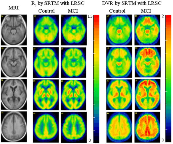
Pixelwise mean of R1 and DVR for control group (n = 28) and MCI group (n = 6). The simplified reference tissue model with linear regression with spatial constraint parametric imaging algorithm was used for generation of R1 and DVR images. The MRI is the normalized mean image across all 34 subjects.
R1(ROI TAC fitting) = 0.99R1(ROI on parametric image) + 0.01 with R2 = 0.98.
Compared to DVR images, R1 images provided gray-white matter contrast consistent with that shown on the MRIs. This suggests that 1) R1 can be used for MRI-PET coregistration; 2) R1 can be used to determine spatial normalization parameters and provide a template for spatial normalization, for both control and MCI groups. Fig. 6 demonstrates that 1) In controls, DVR shows the highest values in thalamus, brain stem, and white matter; 2) The DVRs of mesial temporal cortex, thalamus, occipital cortex, brain stem, and white matter were similar in the control and MCI groups, and 3) The DVRs of caudate, putamen, and cortical regions, including frontal, lateral temporal, parietal and cingulate, in the MCI group were higher than those in the control group. The quantitative comparison of estimates between control and MCI groups is given in the following section.
Comparison of estimates between control and MCI groups
The comparison of ROI estimates between control and MCI groups is summarized in Table. 1. The R1 and k′2R estimates from the control group were similar to those from the MCI group. The DVR estimates from RTM3P were significantly greater than 1 (or BP > 0) in control and MCI groups for all 15 ROIs. However, the DVR estimates from Logan plots were not significant greater than 1 (or BP > 0) in mesial temporal cortex for both control and MCI groups (p = 0.052 and 0.24 for control and MCI, respectively), and not significantly greater than 1 (or BP > 0) in prefrontal cortex for the control group (p = 0.057). The difference in DVR between control and MCI groups was consistent across different estimates. Based on RTM3P, the DVRs in frontal and cingulate cortex for the MCI group were 38% higher on average than those for the control group. The DVRs in caudate, putamen, and lateral temporal cortex for the MCI group was 25% higher on average than those for the control group. There were no significant differences in DVRs between the control and MCI groups for thalamus, mesial temporal cortex, occipital cortex, pons, midbrain and white matter, although there was a trend for the DVR for thalamus to be higher in the MCI compared to control group (p = 0.11). Similar statistical inferences were also obtained for Logan plot and parametric image approaches.
Table 1.
Statistics of ROI based estimates for control (n=28) and MCI (n=6) groups
| Estimates | Group | ROI | 1 | 2 | 3 | 4 | 5 | 6 | 7 | 8 | 9 | 10 | 11 | 12 | 13 | 14 | 15 |
|---|---|---|---|---|---|---|---|---|---|---|---|---|---|---|---|---|---|
| R1 by RTM3P with coupling | Control | Mean | 0.98 | 1.15 | 1.17 | 0.81 | 0.74 | 0.79 | 0.83 | 0.92 | 0.86 | 0.82 | 0.79 | 0.93 | 0.92 | 0.89 | 0.45 |
| SD | 0.07 | 0.05 | 0.06 | 0.06 | 0.06 | 0.05 | 0.06 | 0.07 | 0.06 | 0.05 | 0.06 | 0.09 | 0.05 | 0.06 | 0.04 | ||
| MCI | Mean | 0.96 | 1.15 | 1.17 | 0.79 | 0.74 | 0.80 | 0.83 | 0.91 | 0.86 | 0.79 | 0.80 | 0.92 | 0.96 | 0.93 | 0.43 | |
| SD | 0.08 | 0.09 | 0.07 | 0.03 | 0.05 | 0.02 | 0.04 | 0.10 | 0.04 | 0.04 | 0.05 | 0.09 | 0.05 | 0.04 | 0.06 | ||
| t test | p | 0.62 | 0.97 | 0.91 | 0.22 | 0.85 | 0.83 | 0.87 | 0.67 | 0.91 | 0.21 | 0.63 | 0.69 | 0.17 | 0.10 | 0.64 | |
| k′2R by RTM3P with coupling | Control | Mean | 0.05 (range 0.03 - 0.08) | ||||||||||||||
| SD | 0.01 | ||||||||||||||||
| MCI | Mean | 0.05 (range 0.04 - 0.06) | |||||||||||||||
| SD | 0.01 | ||||||||||||||||
| t test | P | 0.42 | |||||||||||||||
| DVR by RTM3P with coupling | Control | Mean | 1.20 | 1.30 | 1.37 | 1.12 | 1.05 | 1.14 | 1.12 | 1.12 | 1.16 | 1.12 | 1.24 | 1.25 | 1.65 | 1.61 | 1.69 |
| SD | 0.23 | 0.17 | 0.09 | 0.19 | 0.05 | 0.24 | 0.21 | 0.13 | 0.26 | 0.17 | 0.30 | 0.28 | 0.10 | 0.13 | 0.22 | ||
| MCI | Mean | 1.55 | 1.59 | 1.51 | 1.38 | 1.12 | 1.53 | 1.52 | 1.17 | 1.63 | 1.43 | 1.79 | 1.82 | 1.65 | 1.57 | 1.72 | |
| SD | 0.32 | 0.23 | 0.18 | 0.24 | 0.13 | 0.20 | 0.26 | 0.14 | 0.31 | 0.20 | 0.35 | 0.37 | 0.12 | 0.14 | 0.11 | ||
| t test | p | 0.04 | 0.02 | 0.11 | 0.05 | 0.27 | 0.00 | 0.01 | 0.49 | 0.01 | 0.01 | 0.01 | 0.01 | 0.91 | 0.49 | 0.65 | |
| DVR by Logan plot (ROI kinetics) | Control | Mean | 1.20 | 1.32 | 1.32 | 1.12 | 1.03 | 1.14 | 1.09 | 1.20 | 1.17 | 1.16 | 1.25 | 1.30 | 1.60 | 1.54 | 1.47 |
| SD | 0.23 | 0.18 | 0.09 | 0.21 | 0.08 | 0.27 | 0.25 | 0.14 | 0.27 | 0.18 | 0.28 | 0.26 | 0.09 | 0.11 | 0.11 | ||
| MCI | Mean | 1.55 | 1.60 | 1.46 | 1.40 | 1.09 | 1.56 | 1.55 | 1.24 | 1.63 | 1.46 | 1.75 | 1.82 | 1.59 | 1.50 | 1.42 | |
| SD | 0.33 | 0.23 | 0.17 | 0.26 | 0.17 | 0.19 | 0.26 | 0.19 | 0.29 | 0.20 | 0.32 | 0.35 | 0.12 | 0.15 | 0.18 | ||
| t test | p | 0.05 | 0.03 | 0.11 | 0.04 | 0.42 | 0.00 | 0.00 | 0.63 | 0.01 | 0.01 | 0.01 | 0.01 | 0.79 | 0.55 | 0.58 | |
| DVR by Logan plot (parametric image) | Control | Mean | 1.21 | 1.32 | 1.32 | 1.11 | 1.03 | 1.12 | 1.08 | 1.19 | 1.16 | 1.15 | 1.25 | 1.30 | 1.60 | 1.55 | 1.42 |
| SD | 0.23 | 0.18 | 0.09 | 0.20 | 0.08 | 0.27 | 0.25 | 0.13 | 0.26 | 0.18 | 0.27 | 0.26 | 0.09 | 0.10 | 0.11 | ||
| MCI | Mean | 1.55 | 1.60 | 1.46 | 1.39 | 1.09 | 1.54 | 1.54 | 1.23 | 1.62 | 1.45 | 1.75 | 1.82 | 1.59 | 1.51 | 1.39 | |
| SD | 0.31 | 0.23 | 0.17 | 0.26 | 0.17 | 0.19 | 0.26 | 0.18 | 0.29 | 0.20 | 0.32 | 0.36 | 0.12 | 0.15 | 0.17 | ||
| t test | p | 0.04 | 0.03 | 0.11 | 0.04 | 0.42 | 0.00 | 0.01 | 0.63 | 0.01 | 0.01 | 0.01 | 0.01 | 0.88 | 0.57 | 0.72 | |
| DVR by SRTM with LRSC (parametric image) | Control | Mean | 1.19 | 1.30 | 1.35 | 1.08 | 1.00 | 1.05 | 1.04 | 1.11 | 1.12 | 1.08 | 1.20 | 1.24 | 1.58 | 1.53 | 1.38 |
| SD | 0.23 | 0.17 | 0.08 | 0.20 | 0.07 | 0.27 | 0.25 | 0.13 | 0.27 | 0.18 | 0.28 | 0.27 | 0.08 | 0.10 | 0.11 | ||
| MCI | Mean | 1.53 | 1.58 | 1.47 | 1.37 | 1.07 | 1.48 | 1.50 | 1.15 | 1.60 | 1.42 | 1.73 | 1.80 | 1.58 | 1.50 | 1.38 | |
| SD | 0.31 | 0.24 | 0.17 | 0.27 | 0.17 | 0.22 | 0.27 | 0.17 | 0.32 | 0.21 | 0.34 | 0.38 | 0.13 | 0.14 | 0.17 | ||
| t test | p | 0.04 | 0.03 | 0.13 | 0.05 | 0.39 | 0.00 | 0.01 | 0.60 | 0.01 | 0.01 | 0.01 | 0.01 | 1.00 | 0.61 | 1.00 | |
Notes: ROIs are numbered as: 1: caudate, 2: putamen, 3: thalamus, 4: lateral temporal, 5: mesial temporal, 6: obital frontal, 7: prefrontal, 8: occipital, 9: superior frontal, 10: parietal, 11: anterior cingulate, 12: posterior cingulate, 13: pons, 14: midbrain, 15: white matter. The p values were obtained from the 2-sided t test.
Discussion
Three reference tissue models, RTM3P, RTM4P, and RTM5P, were compared for 28 controls and 6 individuals with MCI, who had been studied using [11C]PIB dynamic PET studies. Compared to the RTM3P model, RTM4P and RTM5P models did not yield significant improvements in AIC or estimates. It is notable that these results were based on a sample with relatively low cerebral [11C]PIB specific binding. To generalize this comparison of the three models, it will be important to evaluate the three reference tissue models for [11C]PIB PET with AD patients in future studies. In general, the performance of reference tissue models is dependent on the tracer kinetics in target tissue and reference tissue. For example, the underestimation of BP from SRTM was significantly reduced by a reference tissue model derived from 1 compartment for target tissue and 2 compartments for reference tissue (equivalent to RTM5P) in [11C]carfentanil (Endres et al., 2003) and [11C]diprenorphine dynamic PET studies (Zhou et al., 2006c). As compared to a 2-tissue compartment model with plasma input, the underestimation of [11C]flumazenil BP estimates was (15 ± 0.6)%, (1 ± 1)%, and (15 ± 0.5)%, for RTM3P, RTM4P, and RTM5P respectively (Zhou et al., 2006c).
Variability in the estimates of DVR and k′2R was noticeably reduced by the simultaneous fitting approach. Simultaneous fitting of multiple ROI TACs to the model of coupled parameters can be viewed as an approach that applies spatial constraints in parametric space to the model fitting in kinetic space at the ROI level (Zhou et al., 2002, 2003). However, as the DVR increases, for example in tissues with high density of Aβ, these improvements tend to be smaller. In other words, the DVR estimates from the conventional SRTM (R1, k2, BP) model fitting tend to be similar to those from RTM3P(R1, k′2R, BP) with simultaneous fitting methods if DVR ≫1 (e.g., DVR ≥ 2 or BP ≥ 1).
To compare the data from our study to previous results, a concentration ratio (CR) based semi-quantitative method was applied to the measured dynamic PET data for DVR estimates. As demonstrated by Fig. 8, the DVR estimated by CR was more sensitive to the pre-determined time frame. Consistent with TACs in Fig. 6, the mean of first 20 min scan [11C]PIB images appears to be an appropriate time frame in trade off between contrast (gray matter versus white matter) or structural information and image noise level. The spatial distribution of CR images tends to be stable in time frames after 40 min post tracer injection. The CR over frames from 40 to 90 minutes is higher (13 ± 9)% than the DVR estimated from the Logan plot. However, the CR and Logan plot are highly correlated:
Fig. 8.
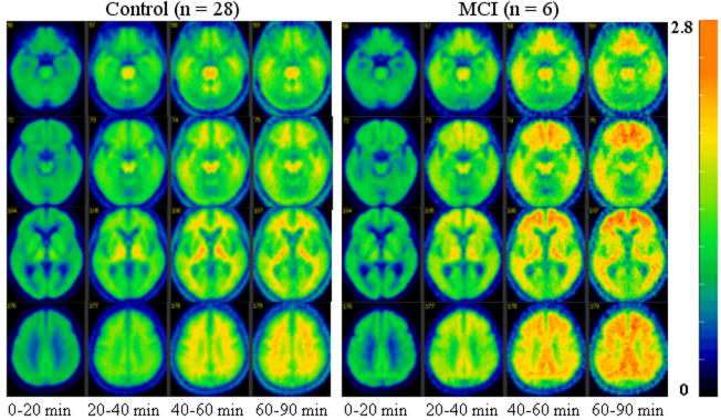
The mean images of concentration ratio images (= target(pixel)/cerebellum (ROI)) for the time periods [0 20] to [60 90] for the control (n = 28) and MCI (n = 6) groups.
CR([40 90]) = 1.39 DVR(Logan plot) − 0.33 (R2 = 0.94).
The ROI based kinetic analysis showed that the statistical power to distinguish between control and MCI group for CR([40 90]) method is the same as that for the Logan plot and the RTM3P or SRTM model. These results were quite consistent with previous results (Lopresti et al., 2006).
It is important to note that [11C]PIB kinetics are different or even opposite to those for FDG in terms image contrast and noise. As shown by Fig. 8 and TACs in Fig. 6, the images obtained with time frame [40 90] are of high noise levels, and the contrast between gray matter and white matter is not consistent with that in early phase [0 20]. Thus, images obtained in later time phase (such as [40 60] or [40 90]) are not appropriate for multi-modality image coregistration. Due to heterogeneity and uncertainty in [11C]PIB in spatial accumulation over brain tissues in MCI or AD patients, and less structural information, the CR images from the later phase are not recommended for use in spatial normalization or as a template. Fig. 9 showed that the statistical power to distinguish between controls and MCI individuals by DVR estimates from RTM3P fitting tends to be stable if PET study time is more than 60 min. The difference in DVR from RTM3P between 60 min and 90 min study is less than 4% in the ROIs including caudate, putamen, thalamus, cortex, pons and midbrain for both controls and MCI. Compared to a 90 min study, the DVR in white matter from a 60 min study is higher by 12% for controls and 10% for MCI group on average. In addition to DVR estimates from RTM3P, the R1 estimates from SRTM model with linear regression provide relative tracer transport rate (from blood) information, and R1 images appear reliable for MRI-PET coregistration and spatial normalization. Taking these factors into consideration, the reference tissue model RTM3P is suggested for kinetic analysis, especially where shorter (< 90 min) PET imaging times are required.
Fig. 9.

The p values for t-tests between control and MCI groups as a function of PET study time. The t-tests are based on the DVR estimates from the RTM3P model with the simultaneous fitting method. The regions of interest (ROIs) are numbered as: 1: caudate, 2: putamen, 3: thalamus, 4: lateral temporal, 5: mesial temporal, 6: obital frontal, 7: prefrontal, 8: occipital, 9: superior frontal, 10: parietal, 11: anterior cingulate, 12: posterior cingulate, 13: pons, 14: midbrain, 15: white matter.
In summary, reference tissue models with parameter coupling were derived and implemented by simultaneous model fitting for ROI kinetic analysis. A previously developed parametric imaging algorithm, linear regression with spatial constraint for the SRTM model, was evaluated. For comparison, the Logan plot with reference tissue input was applied to both ROI kinetic analysis and parametric imaging. Twenty eight controls and six MCI participants, imaged with [11C]PIB dynamic PET, were evaluated in this study. Compared to conventional individual ROI TAC fitting, the variation of DVR estimates was reduced by the simultaneous ROI fitting approach, especially in tissues of low or negligible specific binding in this group of individuals with generally low PIB retention. There were no significant differences in both ROI TAC fitting and DVR estimates between the RTM3P and the RTM4P or RTM5P with simultaneous fitting for parameter estimation. As it produces similar results to the more complex RTM4P and RTM5P models, the simpler RTM3P model is proposed for ROI TAC based kinetic analysis in studies using [11C]PIB PET. Thus, we compared the R1 and DVR images generated by the SRTM with LRSC algorithm to those from the RTM3P ROI kinetic analysis and the DVR images from Logan plot. The RTM3P with simultaneous fitting method is shown to be a robust compartmental modeling approach that may be useful in [11C]PIB PET studies to detect early markers of Alzheimer’s disease where specific ROIs have been hypothesized, especially in situtations where PIB retention is not high. In addition, the SRTM with LRSC algorithm is recommended for generation of R1 and DVR images for pixel-wise quantification of [11C]PIB dynamic PET.
Acknowledgments
We thank the cyclotron, PET, and MRI imaging staff of the Johns Hopkins Medical Institutions; Andrew H. Crabb for data transfer and computer administration. This study was supported in part by the Intramural Research Program, National Institute on Aging, NIH and by N01-AG-3-2124. This work was presented in part at The 53nd Society of Nuclear Medicine Annual Conference, June 3-7, 2006, San Diego, California, U.S.A.
Footnotes
Publisher's Disclaimer: This is a PDF file of an unedited manuscript that has been accepted for publication. As a service to our customers we are providing this early version of the manuscript. The manuscript will undergo copyediting, typesetting, and review of the resulting proof before it is published in its final citable form. Please note that during the production process errors may be discovered which could affect the content, and all legal disclaimers that apply to the journal pertain.
References
- Akaike H. An information criteria (AIC) Math Sci. 1976;14:5–9. [Google Scholar]
- Alpert NM, Badgaiyan RD, Livni E, Fischman AJ. A novel method for noninvasive detection of neuromodulatory changes in specific neurotransmitter systems. Neuroimage. 2003;19(3):1049–1060. doi: 10.1016/s1053-8119(03)00186-1. [DOI] [PubMed] [Google Scholar]
- Blessed G, Tomlinson BE, Roth M. The association between quantitative measures of dementia and senile change in the cerebral gray matter of elderly subjects. Br J Psychiatry. 1968;114:797–811. doi: 10.1192/bjp.114.512.797. [DOI] [PubMed] [Google Scholar]
- Buck A, Westera G, vonSchulthess GK, Burger C. Modeling alternatives for cerebral carbon-11-iomazenil kinetics. J Nucl Med. 1995 1996 Apr;37(4):699–705. [PubMed] [Google Scholar]
- Buckner RL, Snyder AZ, Shannon BJ, LaRossa G, Sachs R, Fotenos AF, Sheline YI, Klunk WE, Mathis CA, Morris JC, Mintun MA. Molecular, structural, and functional characterization of Alzheimer’s disease: evidence for a relationship between default activity, amyloid, and memory. J Neurosci. 2005;25(34):7709–17. doi: 10.1523/JNEUROSCI.2177-05.2005. [DOI] [PMC free article] [PubMed] [Google Scholar]
- Cunningham VJ, Hume SP, Price GR, Ahier RG, Cremer JE, Jones AK. Compartmental analysis of diprenorphine binding to opiate receptors in the rat in vivo and its comparison with equilibrium data in vitro. J Cereb Blood Flow Metab. 1991;11(1):1–9. doi: 10.1038/jcbfm.1991.1. [DOI] [PubMed] [Google Scholar]
- Edison P, Archer HA, Hinz R, Hammers A, Pavese N, Tai YF, Hotton G, Cutler D, Fox N, Kennedy A, Rossor M, Brooks DJ. Amyloid, hypometabolism, and cognition in Alzheimer disease: an [11C]PIB and [18F]FDG PET study. Neurology. 2007;68(7):501–8. doi: 10.1212/01.wnl.0000244749.20056.d4. [DOI] [PubMed] [Google Scholar]
- Cunningham VJ, Matthews JC, Gunn RN, Rabiner EA, Gee AD. Identification and interpretation of microparameters in neuroreceptor compartmental models. Neuroimage. 2004;22(suppl 2):T13. [Google Scholar]
- Endres CJ, Slifstein M, Frankle G, Talbot PS, Laruelle M. Simultaneous modeling of multiple TACs with parameter coupling can be used to enforce the assumption of uniform non-specific binding when applying reference-tissue models, and potentially improve parameter estimation. 2003. Brain03 and BrainPET′03. J Cereb Blood Flow Metab. 2003;23(suppl) [Google Scholar]
- Fagan AM, Mintun MA, Mach RH, Lee SY, Dence CS, Shah AR, Larossa GN, Spinner ML, Klunk WE, Mathis CA, Dekosky ST, Morris JC, Holtzman DM. Inverse relation between in vivo amyloid imaging load and cerebrospinal fluid Abeta(42) in humans. Ann Neurol. 2006;59(3):512–9. doi: 10.1002/ana.20730. [DOI] [PubMed] [Google Scholar]
- Gamaldo A, Moghekar A, Kilada S, Resnick SM, Zonderman AB, O’Brien R. Effect of a clinical stroke on the risk of dementia in a prospective cohort. Neurology. 2006;67(8):1363–1369. doi: 10.1212/01.wnl.0000240285.89067.3f. [DOI] [PubMed] [Google Scholar]
- Ginovart N, Wilson AA, Meyer JH, Hussey D, Houle S. Positron emission tomography quantification of [(11)C]-DASB binding to the human serotonin transporter: modeling strategies. J Cereb Blood Flow Metab. 2001;21(11):1342–1253. doi: 10.1097/00004647-200111000-00010. [DOI] [PubMed] [Google Scholar]
- Gunn RN, Gunn SR, Cunningham VJ. Positron emission tomography compartmental models. J Cereb blood Flow Metab. 2001;21:635–652. doi: 10.1097/00004647-200106000-00002. [DOI] [PubMed] [Google Scholar]
- Gunn RN, Gunn SR, Turkheimer FE, Aston JA, Cunningham VJ. Positron emission tomography compartmental models: a basis pursuit strategy for kinetic modeling. J Cereb Blood Flow Metab. 2002;22(12):1425–39. doi: 10.1097/01.wcb.0000045042.03034.42. [DOI] [PubMed] [Google Scholar]
- Herholz K, Wienhard K, Heiss W-D. Validity of PET studies in brain tumors. Cerebrovascular and Brain Metabolism Review. 1990;2:240–265. [PubMed] [Google Scholar]
- Huang SC, Barrio JR, Phelps ME. Neuroreceptor assay with positron emission tomography: equilibrium versus dynamic approaches. J Cereb Blood Flow Metab. 1986;6(5):515–521. doi: 10.1038/jcbfm.1986.96. [DOI] [PubMed] [Google Scholar]
- Kemppainen NM, Aalto S, Wilson IA, Nagren K, Helin S, Bruck A, Oikonen V, Kailajarvi M, Scheinin M, Viitanen M, Parkkola R, Rinne JO. Voxel-based analysis of PET amyloid ligand [11C]PIB uptake in Alzheimer disease. Neurology. 2006;67(9):1575–80. doi: 10.1212/01.wnl.0000240117.55680.0a. [DOI] [PubMed] [Google Scholar]
- Kimura Y, Hsu H, Toyama H, Senda M, Alpert NM. Improved signal-to-noise ratio in parametric images by cluster analysis. Neuroimage. 1999;9(5):554–61. doi: 10.1006/nimg.1999.0430. [DOI] [PubMed] [Google Scholar]
- Klunk WE, Engler H, Nordberg A, Wang Y, Blomqvist G, Holt DP, Bergstrom M, Savitcheva I, Huang GF, Estrada S, Ausen B, Debnath ML, Barletta J, Price JC, Sandell J, Lopresti BJ, Wall A, Koivisto P, Antoni G, Mathis CA, Langstrom B. Imaging brain amyloid in Alzheimer’s disease with Pittsburgh Compound-B. Ann Neurol. 2004;55(3):306–19. doi: 10.1002/ana.20009. [DOI] [PubMed] [Google Scholar]
- Klunk WE, Lopresti BJ, Ikonomovic MD, Lefterov IM, Koldamova RP, Abrahamson EE, Debnath ML, Holt DP, Huang GF, Shao L, DeKosky ST, Price JC, Mathis CA. Binding of the positron emission tomography tracer Pittsburgh compound-B reflects the amount of amyloid-beta in Alzheimer’s disease brain but not in transgenic mouse brain. J Neurosci. 2005;25(46):10598–606. doi: 10.1523/JNEUROSCI.2990-05.2005. [DOI] [PMC free article] [PubMed] [Google Scholar]
- Kropholler MA, Boellaard R, Schuitemaker A, Folkersma H, van Berckel BN, Lammertsma AA. Evaluation of reference tissue models for the analysis of [(11)C](R)-PK11195 studies. J Cereb Blood Flow Metab. 2006 doi: 10.1038/sj.jcbfm.9600289. in press. [DOI] [PubMed] [Google Scholar]
- Koeppe RA, Holthoff VA, Frey KA, Kilbourn MR, Kuhl DE. Compartmental analysis of [11C]flumazenil kinetics for the estimation of ligand transport rate and receptor distribution using positron emission tomography. J Cereb Blood Flow Metab. 1991;11:735–744. doi: 10.1038/jcbfm.1991.130. [DOI] [PubMed] [Google Scholar]
- Lammertsma AA, Bench CJ, Hume SP, Osman S, Gunn K, Brooks DJ, Frackowiak RSJ. Comparison of Methods for Analysis of Clinical [11C]Raclopride Studies. J Cereb blood Flow Metab. 1996a;16:42–52. doi: 10.1097/00004647-199601000-00005. [DOI] [PubMed] [Google Scholar]
- Lammertsma AA, Hume SP. Simplified reference tissue model for PET receptor studies. NeuroImage. 1996;4:153–158. doi: 10.1006/nimg.1996.0066. [DOI] [PubMed] [Google Scholar]
- Logan J, Fowler JS, Volkow ND, et al. Graphical analysis of reversible radioligand binding from time-activity measurements applied to [N-11C-methuyl]-(-)-cocaine PET studies in human subjects. J Cereb blood Flow Metab. 1990;10:740–747. doi: 10.1038/jcbfm.1990.127. [DOI] [PubMed] [Google Scholar]
- Logan J, Fowler JS, Volkow ND, Wang G-J, Ding Y-S, Alexoff DL. Distribution volume ratios without blood sampling from graphic analysis of PET data. J Cereb Blood Flow Metab. 1996;16:834–840. doi: 10.1097/00004647-199609000-00008. [DOI] [PubMed] [Google Scholar]
- Lopresti BJ, Klunk WE, Mathis CA, Hoge JA, Ziolko SK, Lu X, Meltzer CC, Schimmel K, Tsopelas ND, DeKosky ST, Price JC. Simplified quantification of Pittsburgh Compound B amyloid imaging PET studies: a comparative analysis. J Nucl Med. 2005;46(12):1959–72. [PubMed] [Google Scholar]
- McKhann G, Drachman D, Folstein M, Katzman R, Price D, Stadlan EM. Clinical diagnosis of Alzheimer’s disease: report of the NINCDS-ADRDA Work Group under the auspices of Department of Health and Human Services Task Force on Alzheimer’s Disease. Neurology. 1984;34(7):939–44. doi: 10.1212/wnl.34.7.939. [DOI] [PubMed] [Google Scholar]
- Mathis CA, Wang Y, Holt DP, Huang GF, Debnath ML, Klunk WE. Synthesis and evaluation of 11C-labeled 6-substituted 2-arylbenzothiazoles as amyloid imaging agents. Med Chem. 2003;46(13):2740–54. doi: 10.1021/jm030026b. [DOI] [PubMed] [Google Scholar]
- Mathis CA, Wang Y, Klunk WE. Imaging beta-amyloid plaques and neurofibrillary tangles in the aging human brain. Curr Pharm Des. 2004;10(13):1469–92. doi: 10.2174/1381612043384772. [DOI] [PubMed] [Google Scholar]
- Mathis CA, Klunk WE, Price JC, DeKosky ST. Imaging technology for neurodegenerative diseases: progress toward detection of specific pathologies. Arch Neurol. 2005;62(2):196–200. doi: 10.1001/archneur.62.2.196. [DOI] [PubMed] [Google Scholar]
- Marquardt DW. An algorithm for least-squares estimations of nonlinear parameters. J Soc Ind App Math. 1963;11:431–441. [Google Scholar]
- Millet P, Graf C, Buck A, Walder B, Ibanez V. Evaluation of the reference tissue models for PET and SPECT benzodiazepine binding parameters. Neuroimage. 2002;17(2):928–942. [PubMed] [Google Scholar]
- Mintun MA. Utilizing advanced imaging and surrogate markers across the spectrum of Alzheimer’s disease. CNS Spectr. 2005;10(11 Suppl 18):13–6. doi: 10.1017/s1092852900014188. [DOI] [PubMed] [Google Scholar]
- Mintun MA, Raichle ME, Kilbourn MR, Wooten GF, Welch MJ. A quantitative model for the in vivo assessment of drug binding sites with positron emission tomography. Ann Neurol. 1984;15:217–227. doi: 10.1002/ana.410150302. [DOI] [PubMed] [Google Scholar]
- Mintun MA, Larossa GN, Sheline YI, Dence CS, Lee SY, Mach RH, Klunk WE, Mathis CA, DeKosky ST, Morris JC. [11C]PIB in a nondemented population: potential antecedent marker of Alzheimer disease. Neurology. 2006;67(3):446–52. doi: 10.1212/01.wnl.0000228230.26044.a4. [DOI] [PubMed] [Google Scholar]
- Morris ED, Yoder KK, Wang C, Normandin MD, Zheng QH, Mock B, Muzic RF, Jr, Froehlich JC. ntPET: a new application of PET imaging for characterizing the kinetics of endogenous neurotransmitter release. Mol Imaging. 2005;4(4):473–89. doi: 10.2310/7290.2005.05130. [DOI] [PubMed] [Google Scholar]
- Morris JC, Storandt M, Miller JP, McKeel DW, Price JL, Rubin EH, Berg L. Mild cognitive impairment represents early-stage Alzheimer disease. Arch Neurol. 2001;58(3):397–405. doi: 10.1001/archneur.58.3.397. [DOI] [PubMed] [Google Scholar]
- Nichols L, Pike VW, Cai L, Innis RB. Imaging and in vivo quantitation of β-amyloid: an exemplary biomarker for Alzheimer’s disease? Biol Psychiatry. 2006;59(10):940–947. doi: 10.1016/j.biopsych.2005.12.004. [DOI] [PubMed] [Google Scholar]
- Nordberg A. PET imaging of amyloid in Alzheimer’s disease. Lancet Neurol. 2004;3(9):519–527. doi: 10.1016/S1474-4422(04)00853-1. [DOI] [PubMed] [Google Scholar]
- Price JC, Klunk WE, Lopresti BJ, Lu X, Hoge JA, Ziolko SK, Holt DP, Meltzer CC, DeKosky ST, Mathis CA. Kinetic modeling of amyloid binding in humans using PET imaging and Pittsburgh Compound-B. J Cereb Blood Flow Metab. 2001;2005;25(11):1528–47. doi: 10.1038/sj.jcbfm.9600146. [DOI] [PubMed] [Google Scholar]
- Raylman RR, Hutchins GD, Beanlands RS, Schwaiger M. Modeling of carbon-11-acetate kinetics by simultaneously fitting data from multiple ROIs coupled by common parameters. J Nucl Med. 1994 May;35(5):909–13. [PubMed] [Google Scholar]
- Reimold M, Mueller-Schauenburg W, Becker GA, Reischl G, Dohmen BM, Bares R. Non-invasive assessment of distribution volume ratios and binding potential: tissue heterogeneity and interindividually averaged time-activity curves. Eur J Nucl Med Mol Imaging. 2004;31(4):564–77. doi: 10.1007/s00259-003-1389-5. [DOI] [PubMed] [Google Scholar]
- Resnick SM, Goldszal AF, Davatzikos C, Golski S, Kraut MA, Metter EJ, Bryan RN, Zonderman AB. One-year age changes in MRI brain volumes in older adults. Cereb Cortex. 2000;10(5):464–72. doi: 10.1093/cercor/10.5.464. [DOI] [PubMed] [Google Scholar]
- Resnick SM, Pham DL, Kraut MA, Zonderman AB, Davatzikos C. Longitudinal magnetic resonance imaging studies of older adults: a shrinking brain. J Neurosci. 2003;23(8):3295–301. doi: 10.1523/JNEUROSCI.23-08-03295.2003. [DOI] [PMC free article] [PubMed] [Google Scholar]
- Shoghi-Jadid K, Small GW, Agdeppa ED, Kepe V, Ercoli LM, Siddarth P, Read S, Satyamurthy N, Petric A, Huang SC, Barrio JR. Localization of neurofibrillary tangles and beta-amyloid plaques in the brains of living patients with Alzheimer disease. Am J Geriatr Psychiatry. 2002;10(1):24–35. [PubMed] [Google Scholar]
- Small GW, Kepe V, Ercoli LM, Siddarth P, Bookheimer SY, Miller KJ, Lavretsky H, Burggren AC, Cole GM, Vinters HV, Thompson PM, Huang SC, Satyamurthy N, Phelps ME, Barrio JR. PET of brain amyloid and tau in mild cognitive impairment. N Engl J Med. 2006;355(25):2652–63. doi: 10.1056/NEJMoa054625. [DOI] [PubMed] [Google Scholar]
- Suzuki A, Tashiro M, Kimura Y, Mochizuki H, Ishii K, Watabe H, Yanai K, Ishiwata K, Ishii K. Use of reference tissue models for quantification of histamine H1 receptors in human brain by using positron emission tomography and [11C]doxepin. Ann Nucl Med. 2005;19(6):425–433. doi: 10.1007/BF02985569. [DOI] [PubMed] [Google Scholar]
- Turkheimer FE, Hinz R, Gunn RN, Aston JA, Gunn SR, Cunningham VJ. Rank-shaping regularization of exponential spectral analysis for application to functional parametric mapping. Phys Med Biol. 2003;48(23):3819–41. doi: 10.1088/0031-9155/48/23/002. [DOI] [PubMed] [Google Scholar]
- Turkheimer FE, Hinz R, Cunningham VJ. On the undecidability among kinetic models: from model selection to model averaging. J Cereb blood Flow Metab. 2003;23:490–498. doi: 10.1097/01.WCB.0000050065.57184.BB. [DOI] [PubMed] [Google Scholar]
- Verhoeff NP, Wilson AA, Takeshita S, Trop L, Hussey D, Singh K, Kung HF, Kung MP, Houle S. In-vivo imaging of Alzheimer disease beta-amyloid with [11C]SB-13 PET. Am J Geriatr Psychiatry. 2004;12(6):584–95. doi: 10.1176/appi.ajgp.12.6.584. [DOI] [PubMed] [Google Scholar]
- Votaw JR, Howell LL, Martarello L, Hoffman JM, Kilts CD, Lindsey KP, Goodman MM. Measurement of dopamine transporter occupancy for multiple injections of cocaine using a single injection of [F-18]FECNT. Synapse. 2002;44(4):203–210. doi: 10.1002/syn.10068. [DOI] [PubMed] [Google Scholar]
- Watabe H, Endres CJ, Carson RE. Modeling methods for the determination of dopamine release with [11C]raclopride and constant infusion. Neuroimage. 1998;7:A57. [Google Scholar]
- Wu C, Pike VW, Wang Y. Amyloid imaging: from benchtop to bedside. Curr Top Dev Biol. 2005;70:171–213. doi: 10.1016/S0070-2153(05)70008-9. [DOI] [PubMed] [Google Scholar]
- Wu Y, Carson RE. Noise reduction in the simplified reference tissue model for neuroreceptor functional imaging. J Cereb Blood Flow Metab. 2002;22(12):1440–52. doi: 10.1097/01.WCB.0000033967.83623.34. [DOI] [PubMed] [Google Scholar]
- Zhou Y, Cloughesy T, Hoh CK, Black K, Phelps ME. A modeling-based factor extraction method for determining spatial heterogeneity of Ga-68 EDTA kinetics in brain tumors. IEEE Transactions on Nuclear Science. 1997;44(6):2522–2527. [Google Scholar]
- Zhou Y, Huang SC, Bergsneider M, Wong DF. Improved parametric image generation using spatial-temporal analysis of dynamic PET studies. NeuroImage. 2002;15:697–707. doi: 10.1006/nimg.2001.1021. [DOI] [PubMed] [Google Scholar]
- Zhou Y, Endres CJ, Brasic JR, Huang SC, Wong DF. Linear regression with spatial constraint to generate parametric images of ligand-receptor dynamic PET studies with a simplified reference tissue model. Neuroimage. 2003;18(4):975–989. doi: 10.1016/s1053-8119(03)00017-x. [DOI] [PubMed] [Google Scholar]
- Zhou Y, Chen MK, Endres CJ, Ye W, Brasic JR, Alexander M, Crabb AH, Guilarte TR, Wong DF. An extended simplified reference tissue model for the quantification of dynamic PET with amphetamine challenge. Neuroimage. 2006a;33(2):550–563. doi: 10.1016/j.neuroimage.2006.06.038. [DOI] [PubMed] [Google Scholar]
- Zhou Y, Resnick SM, Ye W, Fan H, Holt D, Klunk WE, Mathis CA, Dannals R, Wong DF. Evaluation of reference tissue models for quantification of [11C] Pittsburgh compound B dynamic PET studies. J Nucl Med. 2006b;47(S1):117P. [Google Scholar]
- Zhou Y, Ye W, Brasic JR, Hilton J, Wong DF. Compartmental model with plasma input versus reference tissue model for quantification of liganreceptor dynamic PET studies. J Nucl Med. 2006c;47(S1):117P. [Google Scholar]