Quantifying the urban environment: a scale measure of urbanicity outperforms the urban-rural dichotomy

Abstract

The rapid urbanization of the developing world has important consequences for human health. Although several authorities have called for better research on the relationships between urbanicity and health, most researchers still use a poor measurement of urbanicity, the urban-rural dichotomy. Our goal was to construct a scale of urbanicity using community level data from the Cebu Longitudinal Health and Nutrition Survey. We used established scale development methods to validate the new measure and tested its performance against the dichotomy. The new scale illustrated misclassification by the urban-rural dichotomy, and was able to detect differences in urbanicity, both between communities and across time, that were not apparent before. Furthermore, using a continuous measure of urbanicity allowed for better illustrations of the relationships between urbanicity and health. The new scale is a better measure of urbanicity than the traditionally used urban-rural dichotomy.

INTRODUCTION

"Over the last 50 years, the world has witnessed a dramatic growth of its urban population. The speed and the scale of this growth, especially concentrated in the less developed regions, continue to pose formidable challenges to the individual countries as well as to the world community. Monitoring these developments and creating sustainable urban environments remain crucial issues on the international development agenda." - United Nations Department of Economic and Social Affairs/Population Division (UN, 2004)

Urbanization is a key force in human society, so much so that McMichael (2000) suggests that city-living may be the "keystone of human ecology" (p. 1123) , a point well illustrated by rapid rates of urbanization across the globe. McMichael also praises cities themselves as centers of "ideas, energy, creativity and technology" (p. 1123). This characterization of the "city", coupled with the inextricable link between urbanization and development (Kasarda & Crenshaw, 1991), has led many to idealize city-living. But city-living has important effects on health, both good and bad. Benefits of city-life include better access to heath care, education, and social support, as well as improved water and sanitation infrastructure (McMichael, 2000; Vlahov & Galea, 2002). Adverse effects include poor physical activity and dietary habits, high prevalence of various infectious and chronic diseases, exposure to environmental pollution, poor mental health, increased tobacco, alcohol, and drug use, higher risk of injury, and higher crime rates (Ghassemi, Harrison, & Mohammad, 2002; Gracey, 2002; Keiser, Utzinger, Caldas de Castro, Smith, Tanner, & Singer, 2004; McMichael, 2000; Montgomery, Stren, Cohen, & Reed, 2003; Mutatkar, 1995; Popkin, 2001; Popkin & Gordon-Larsen, 2004; Vlahov & Galea, 2002; Vorster, 2002).

Further complicating urban-health, the rapid urbanization now seen in the developing world is often characterized by the development of peri-urban squatter settlements, also commonly referred to as slums or shantytowns (Harpham & Stephens, 1991; Wang'ombe, 1995; Yach, Mathews, & Buch, 1990). Within these peri-urban areas, poverty, crowding, environmental pollutants, a lack of services, and poor housing combine to create a particularly unhealthy environment, exposing their inhabitants to the "worst of both the traditional and modern world" (McMichael, 2000). Thus, city-dwellers in rapidly urbanizing countries may face a double burden of disease, similar to the "urban penalty" seen in Europe after the industrial revolution when city-dwellers suffered from worse health than their rural counterparts. Although the health of urban populations generally fares better than that of rural populations, there is evidence that the health of poor, urban populations can be worse than some rural populations (Montgomery et al., 2003). These connections between rapid urbanization, urban life, and health have led several authorities to call for more urban-health research (Gracey, 2002; Montgomery et al., 2003; Vlahov & Galea, 2002).

Good empirical research starts with the valid measurement of all relevant variables. Urbanization is typically defined as the proportion of a given population living in an area classified as “urban” (Davis, 1965). However, in studies of urban environments and health, what we are really interested in is the nature of urban environments, an admittedly broad concept that is often referred to as urbanicity (alternatively termed urban-ness or urbanism). Investigators typically use the urban-rural dichotomy to describe urbanicity. The dominance of the urban-rural dichotomy dates at least as far back as the 1940s when the UN began reporting statistics on world urbanization trends, and the dichotomy continues to be the principal form of urban categorization used by the United Nations Population Division (Champion & Hugo, 2004).

The dichotomy, while expedient and often useful, has been previously recognized as inadequate (Champion & Hugo, 2004; McDade & Adair, 2001; Mendez, Stookey, Adair, & Popkin, 2004; Vlahov & Galea, 2002; Yach et al., 1990). One major problem is that there is no universally used definition of "urban" or "rural". Vlahov and Galea (2002) illustrate this point nicely, noting that "among 228 countries for which the United Nations has data, about half use administrative definitions of urban (e.g., living in the capital city), 51 use [population] size and density, 39 use functional characteristics (e.g., economic activity), 22 have no definition of urban, and 8 define all (e.g., Singapore) or none (e.g., Polynesian countries) of their population as urban" (p. 54).

That nations define "urban" differently hints at the underlying problem with the dichotomy; urbanicity is too complex to measure so simply. In the past, urban and rural environments were clearly different, but modern "rural" areas are now experiencing factors traditionally associated with the urban environment and the result is "increased blurring of urban-rural distinctions" (Champion & Hugo, 2004). Additionally, patterns of urbanization vary between regions (Kasarda & Crenshaw, 1991), resulting in equally varied settlement types and a great deal of heterogeneity among urban areas across the globe and even within countries (Champion & Hugo, 2004). The importance of this heterogeneity is not lost on urban health researchers, many of whom have called for more intra- and inter-urban health research (McDade & Adair, 2001; Vlahov & Galea, 2002; Wharton, 2002; Yach et al., 1990).

Although the inadequacies of the urban-rural dichotomy have been recognized for some time, most health researchers still rely on it almost exclusively. Some alternative measurements are worth noting here: the use of remote sensing to measure urbanicity (Tatem & Hay, 2004; Weeks, Getis, Hill, Gadalla, & Rashed, 2004); a survey instrument to measure the built environment (Weich, Burton, Blanchard, Prince, Sproston, & Erens, 2001); an assessment tool for collecting information on urban neighborhood characteristics (Caughy, O'Campo, & Patterson, 2001); and a multidimensional characterization of settlement type based on style and density of housing, predominant commercial and agricultural activities, and access to services (Adair, Vanderslice, & Zohoori, 1993). Also of interest are papers such as Ruel, Haddad and Garrett (1999) which pose hypotheses in the context of specific factors that generally differ between urban and rural environments.

Champion and Hugo (2004) address the question of how to best measure the urban environment in New Forms of Urbanization: Beyond the Urban-Rural Dichotomy. They begin by characterizing the dichotomy as a single-dimension classification system under which environments are dichotomized based on a single factor such as population size, density, or some other factor traditionally recognized as being different for urban and rural environments. Champion and Hugo then suggest that environments could be considered as falling along a continuum of this single factor, and can be categorized as needed by creating cut points along the continuum. The terms "urban" and "rural" then denote opposite ends of this continuum, and every environment would fall somewhere in between.

However, defining urbanicity by only one factor could lead to misclassification since urbanization is a highly variable process which results in diverse settlement patterns. An even more sophisticated classification of environments would place them along a continuum based on more than one factor. To illustrate this, Champion and Hugo (2004) point to work in Indonesia, in which communities are given a score based on population density, the proportion of households engaged in agriculture, and the presence of facilities traditionally associated with urban environments (e.g. school, hospitals, etc.). The sum of these three component scores results in an overall scale ranging from 3–30. Communities which score ≥23 are labeled urban, those scoring ≤17 are classified as rural, and those that fall in the middle are "field checked" and assigned to a category. While Champion and Hugo go on to describe other methods of urban classification, we will continue here with the possibility of using a scale to describe urbanicity.

Building on the work of Stookey (2002) and Mendez, Stookey, Adair & Popkin (2004), our goal was to develop a multi-component scale of urbanicity that would allow us to investigate the effects of urbanicity on child health in a three-country comparative study of China, Russia, and the Philippines. This work is being carried out in the context of a broader research program on urbanization and the nutrition transition (Popkin, 2001). For the Philippines we are using data from the Cebu Longitudinal Health and Nutrition Survey (CLHNS) to investigate how urbanicity has affected the health of study participants living in a rapidly urbanizing metropolitan area over a 20 year period.

We elected to create a scale of urbanicity to replace the urban-rural dichotomy for several reasons. First, scales are developed in an a priori fashion, making them suitable for comparing data from different sources. A scale also allows comparisons of similar measures over time, and analyses of its components can identify specific factors which vary consistently across urbanizing environments. Here we report on the development of a multi-component urbanicity scale for Metro Cebu, the second largest metropolitan region of the Philippines. Given the limited amount of published research using novel measurements of urbanicity, we feel this is a positive addition to our collective knowledge.

METHODS

Study Population and Data

We used data from the CLHNS to develop the scale. The study location, Metro Cebu (population 1.9 million) on the east coast of Cebu Island in the central Philippines, comprises three cities (Cebu City, Mandaue, and Lapu-Lapu), seven municipalities in surrounding peri-urban and rural areas, and a total of 270 administrative units (barangays). Barangays are typically villages in rural areas or neighborhoods in urban areas and average approximately two km² in size. The study area is ecologically diverse, with densely populated barangays in the cities, less dense peri-urban areas and rural towns, and more isolated mountain and island rural areas.

In 1983, a single stage cluster sampling procedure was used to randomly select 17 urban (over-sampled by design) and 16 rural barangays (as defined by the Philippine census using a combination of population characteristics and administrative function). The selected barangays were surveyed for pregnant women in late 1982 and early 1983. Any woman giving birth in a selected barangay from May 1, 1983 to April 30, 1984 was then recruited for the study sample. A baseline survey was conducted with 3,327 pregnant women. Subsequent interviews took place immediately after birth and then at two month intervals for the next 24 months. Follow up surveys were conducted in 1991, 1994, 1998, and 2002. As a point of information, the 2002 survey located about two thirds of baseline participants. However, we do not present follow-up rates for individual participants because the urbanicity scale is based on community data, and our brief illustration of the utility of the scale in predicting health-related behaviors uses only baseline data.

Community level data were also collected for each round of the survey. The community surveys include information on the barangays' physical characteristics, infrastructure and utilities, social services, community organizations, industrial and commercial establishments, labor markets, and wage rates. Data for the community surveys were obtained from barangay officials or other knowledgeable people recommended by these officials. While the study participants initially lived in 33 barangays, participants in the 2002 survey lived in 183 different barangays (due to movement within the Metro Cebu area). Community level data exist for every barangay in which a study participant lived for each survey year (1983, 1986, 1991, 1994, 1998, and 2002). Since our focus here is on community level change, we only use data from the original 33 barangays (in which more than 80% of our respondents still lived in 2002).

Scale Development

DeVellis (2003) defines a scale as a "collection of items combined into a composite score" that are "intended to reveal levels of theoretical variables not readily observable by direct means" (p. 8–9). In this case, the theoretical (or latent) variable is urbanicity, which cannot be directly measured. To overcome this, a scale takes a collection of items that are thought to co-vary with the latent variable and use them as a proxy measurement.

Item Selection

Items were included in our "urbanicity scale" based on two criteria: content validity (an a priori assessment, based on authoritative sources such as peer-reviewed literature, of whether an item truly reflects urbanicity), and the availability of relevant data for every barangay and survey year in the CLHNS, thus ensuring comparability of the scale over time.

There are several characteristics that researchers generally associate with urbanicity. Cities Transformed (Montgomery et al., 2003) provides a table of factors that typically differ between urban and rural environments which includes (but is not limited to) population density and size, access to education, the range of goods and services available, access to health services, and improved access to water and electricity. Yach, et al. (1990) point to several characteristics of urbanization, including rapid population growth and concentration, and improved access to employment, education, and modern health care. Vlahov and Galea (2002) suggest that urbanicity is defined by the transformations that come about due to changes in population size, density, heterogeneity, and distance from other population centers. They go on to highlight the provision of health and social services, as well as alterations in the social and built environments, as important components of the urban environment. In a factor analysis, McDade and Adair (2001) using data from the CLHNS found that a high population density and the availability of infrastructure and services (telephone, mail, transportation, electricity, water, and health care facilities) were all correlates of urbanicity.

For China, Mendez et al (Mendez et al., 2004) identified 10 components to represent urbanicity (population size and density; housing related infrastructure; transportation infrastructure; health facilities; educational facilities; market availability; communication infrastructure; economic indices; and sanitation). They found that “each component score varied directly and significantly (by linear regression p<0.001) with the overall urbanicity score” (Mendez et al., 2004). Unfortunately, we lacked comparable community level data on housing infrastructure, economic indices, and sanitation, and could not consistently impute the missing community variables from household data due to the small numbers of households surveyed in some barangays. How might this omission affect the validity of the urbanicity scale presented here? A property of a valid scale is that it serves as a proxy for the "missing" items as well as the latent variable (since they are, in theory, also caused by the underlying latent construct the scale is measuring). Because the three components missing from the scale presented here (but that were included in the scale by Mendez et al. (2004)) were highly correlated with the other seven components (used in both scales), we conclude that their inclusion in this scale would not have added any new information to this scale. Taking all of this into consideration, we were left with the following items:

• Population Size

• Population Density

• Communications The presence of phone service, mail, newspapers, the internet, cable TV, and cellular phones

• Transportation The density of paved roads, and the availability of public transportation

• Educational Facilities The presence of educational institutions, including primary and secondary schools, colleges, and vocational schools

• Health Services The presence of health services, including hospitals, medical clinics, maternal health clinics, family planning clinics, and community health centers

• Markets The number of Sari-Sari stores (small, retail shops), and the presence of drug stores, grocery stores, and gas stations

Each component can theoretically take a value from zero to 10, resulting in scale ranging from zero to 70 (item point values in Appendix A). Table one displays the observed mean and range of the urbanicity scale for each survey year, noting the number of barangays surveyed in each year.

Table 1.

Urbanicity Scale Characteristics for Each Year Surveyed.

	Year
	1983	1986	1991	1994	1998	2002
Number of Barangays Surveyed	33	33	170	172	169	183
Mean Urbanicity Score for All Barangays (Range)	23.1 (5–49)	21.7 (4–48)	28.8 (5–59)	30.6 (8–59)	34.1 (8–59)	36.9 (7–60)
Cronbach's Alpha a	.8808	.8879	.8763	.8915	.8757	.8707
Item Scale Correlations b
Population	.7505	.7866	.7819	.8073	.7953	.7247
Population Density	.7390	.7297	.6808	.7256	.7151	.6441
Communication	.8673	.7734	.8037	.8084	.6411	.6978
Transportation	.6463	.6089	.6338	.6479	.5717	.5580
Education	.2532*	.2080**	.3415	.4037	.4539	.4836
Health	.6769	.7705	.6912	.7632	.8125	.7460
Markets	.6793	.8213	.8104	.8383	.8266	.7960

^aDeVellis (2003) describes values falling between .8 and .9 as "very good".

^bUnless otherwise noted, all corrected item-scale correlations are statistically different from zero at a p-value<.001

^*p=0.155,

^**p=.245

It is important to note that the components making up the scale are likely to affect its generalizability. In more developed regions, the scale components just described might not vary appreciably between “urban” and “rural” areas. For example, in the United States, community level access to phone service, mail, newspapers, the internet, cable TV, and cellular phones is nearly universal. Furthermore, the scale cannot be considered as an adequate measure of other dimensions often associated with urban environments, such as social cohesion or crime. These factors may very well be caused by the underlying latent variable that this scale aims to define, but there is no explicit way for us to know this given the available data. However, by clearly describing the components included in the urbanicity scale, we are at least sharing one specific definition of “urbanicity” with other researchers so that more meaningful comparisons can be made between regions and studies.

The following sections document the methods used to validate this scale. Unless otherwise noted, these methods are taken directly from DeVellis (2003).

Assessing Scale Reliability

Scale reliability, as defined by DeVellis (2003), is "the proportion of variance attributed to the true score of the latent variable" (p. 27). When assessing scale reliability we assume that the scale is valid with respect to the latent variable (in this case urbanicity) and are only concerned with how strongly the scale's items are related to each other. Strong relationships among variables can then be attributed to causal relationships among them (unlikely) or to a shared cause (the latent variable). Scale reliability can be assessed by looking at its internal consistency and temporal stability.

Internal Consistency

Internal consistency refers to the degree of inter-relatedness of the items within the scale (DeVellis, 2003). Because a scale is collection of items with a shared cause, the items are expected to correlate with each other. One way to assess the internal consistency of the items is to examine their corrected item-scale correlations (DeVellis, 2003), which are simply the correlations between each item and the collection of remaining items. Table one displays the corrected item-scale correlations for every item, in each year. With the exception of the education component, the correlations (Spearman) are high (>.5) and statistically different from zero (p<.001). For education, the correlations ranged between .2080 and .4836. In 1983 and 1986, the corrected item-scale correlations for education were not statistically different from zero (p>.05). However, education was still included in the scale based on its improved correlations over time, its traditionally recognized relationships with health and urbanicity, and the ideal values observed for the scale's alpha values when education is included.

Cronbach's coefficient alpha is often used as a measure of internal consistency (DeVellis, 2003). It is defined as the proportion of total variation in the scale that is shared. It is calculated as follows:

$$\alpha =\left(\frac{k}{k-1}\right)\left(1-\frac{\Sigma {\sigma }_i^2}{{\sigma }_{yi}^2}\right)$$ (1)

Where k is the number of items in the scale, $\Sigma {\sigma }_i^2$ is the unshared variation among the items, and ${\sigma }_{yi}^2$ is the total variation.

Thus the equation expresses alpha by calculating the proportion of total variance that is unique to each item and subtracting this from one to arrive at proportion of shared variance among components; this difference is then multiplied by a correction factor based on the number of items in the scale. The shared variance is attributed to variation in the theoretical variable, while unshared variance is attributed to error. Thus the greater the proportion of shared variance among scale items, the more likely they are to have a shared cause. DeVellis (2003) suggests that an alpha falling between .8 and .9 as very good for population data. Table one displays the calculated alphas for each survey year. They range from .8707 to .8915, indicating an ideal level of internal consistency among the scale's seven items.

Temporal Stability

Temporal stability can also serve as an indicator of scale reliability (DeVellis, 2003). If a scale is truly representative of an underlying latent variable, then it should consistently assess that latent construct at different points in time (DeVellis, 2003). This is sometimes referred to as test-retest reliability. It also logically follows that the components making up the scale should relate consistently over time. It is important to note that factors other than reliability can affect the temporal stability of a measure. Because DeVellis does not give specific guidelines on statistical testing to assess temporal stability, we made a qualitative assessment of how the scale and it components were related over time.

As shown in table one, the mean urbanicity scores steadily increase for each survey year (with the exception of 1983–1986) which is exactly what we would expect. Spearman correlations among the urbanicity scores across all years were all strong (0.85 to 0.97, p<0.000) and predictably varied as function of time between survey years. Furthermore, the corrected item scale correlations and alphas are generally consistent over time indicating that the scale’s components are similarly related for each survey year (this was also true when the analysis was restricted to the 33 barangays surveyed at baseline). While no decisions about a scale’s reliability should rest solely on its temporal stability, we see nothing to convince us that the scale is not reliable.

Assessing Scale Validity

If reliability helps assure us that the scale items have a shared cause, then the scale's validity tells us whether the cause they share is the one we had in mind when developing the scale. In this case, the theoretically shared variable is urbanicity. DeVellis (2003) refers to three types of validity: content validity, criterion related validity, and construct validity. We will examine all three.

Content Validity

Content validity (DeVellis, 2003) refers to the extent that a set of items truly represent what you intend to measure and not something else. In a perfect world, the subset of items would be randomly selected from an infinite set of items that are known to reflect the latent variable. Because this is an impossible task, the best way available to assess content validity is to choose appropriate items based on a priori knowledge. In our case, the inclusion of each item in the urbanicity scale is supported by multiple authoritative sources (McDade & Adair, 2001; Montgomery et al., 2003; Vlahov & Galea, 2002; Yach et al., 1990).

Criterion Related Validity

Criterion related validity (DeVellis, 2003) is based on the scale's empirical association to a "gold standard." The nature of the relationship (be it causal or otherwise) is not important, just its consistency. Although we have no gold standard, one comparison we can make is between the urbanicity scale for 1983 and a previously defined set of settlement classifications derived from household level data during the same period. These classifications were made by experienced local fieldworkers, who differentiated households into six settlement types based on style and density of housing, predominant commercial and agricultural activities, and access to services. The categories are defined as urban core (high density, at the city center), urban squatter (high density, poor housing and sanitation), peri-urban (lower density, less access to the city center), rural town (services and markets but not contiguous with major cities), rural non-town (low density, access to transportation to more urban areas), and remote (Adair et al., 1993).

Table two illustrates the observed relationship between the scale of urbanicity and the settlement types defined above. The relationship is exactly as we would predict: the urban households were typically located in barangays with high urbanicity scores, and the scores steadily decrease as the household settlement type becomes more rural. It is important to recognize here that the urbanicity scale categorizes urban core and urban squatter as being similar, although we might expect important differences with regards to health.

Table 2.

Means and Ranges of Barangay Urbanicity Scores by Household Settlement Type^* in 1983

	Settlement Type**
	Urban Core	Urban Squatter	Peri-Urban	Rural Town	Rural Non-town	Remote
n households	709	496	743	589	325	325
Mean Urbanicity Score (Range)	41.2 (23–44)	41.9 (17–49)	30.7 (22–42)	26.2 (9–45)	17.2 (6–25)	12.01 (5–27)

^*From Adair et al. (1993)

^**There were 140 household with no data for settlement type. The mean urbanicity score for the barangays these household were located in was 30.85

The urbanicity scale for 1983 was also compared to the 1980 Philippine census classification, with "urban" communities averaging a score of 32.7 (range: 17–49), compared to the "rural" communities which averaged a score of 12.9 (5–27). Similarly, in 2002, communities as defined as "urban" by the 2000 census had an average score of 38.5 (12–59) and "rural" communities had an average score of 14.14 (9–24). These scores fall in line with values we would expect, comparing urban to rural, and 1983 to 2002.

Construct Validity

Construct validity is "directly concerned with the theoretical relationship of a variable (e.g., a score on some scale) to other variables" (DeVellis, 2003). In other words, the scale should behave in a way that's consistent with the underlying theoretical variable.

For instance, in the context of the nutrition transition, it generally true that urban dwellers consume more calories and a higher percentage of calories from fat than rural residents (Popkin, 2001). This would be particularly true at stage four of the transition (Popkin & Gordon-Larsen, 2004), when urbanites are first exposed to the "western" diet, which would be the case in the Philippines over the past 20 years. Figures one and two are scatter plots of total caloric intake or percentage of calories from fat (as measured by 24 hour dietary recalls in the study population) and the urbanicity scale, with a lowess plot to indicate trend. Both illustrate that the observed relationship between diet and the urbanicity scale are what we would predict: total calories consumed and the percentage of diet from fat increase as the urbanicity score increases.

Figure 1.

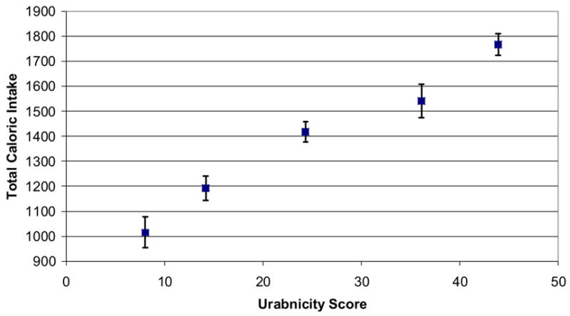
Mean Total Caloric Intake (and 95% CI) in Study Mothers by Quintile of Urbanicity in 1983

Figure 2.

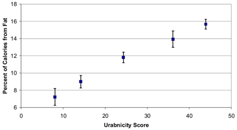
Mean Percent Fat Intake (and 95% CI) in Study Mothers by Quintile of Urbanicity in 1983

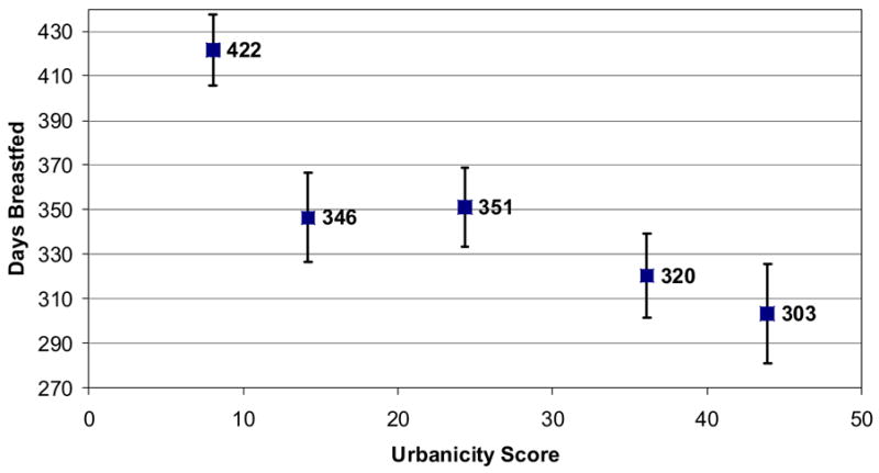
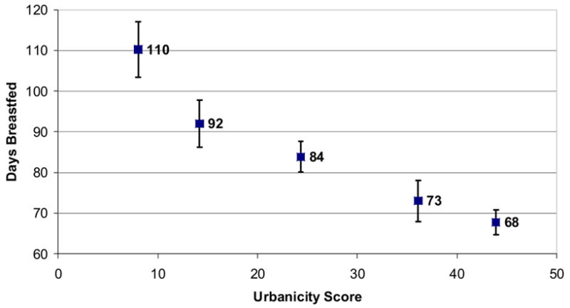
We also compared the urbanicity scale to breastfeeding behavior in the study population. It is well documented in a variety of developing countries that rural mothers tend to breastfeed their children to older ages than urban mothers (Giashuddin & Kabir, 2004; Perez-Escamilla, 2003). Figures three and four show the average age in days at which children stopped "any" and "exclusive" breastfeeding by quintile of the urbanicity scale (with each quintile plotted along the x axis by its mean urbanicity value). The predicted relationship, that rural mothers exclusively breastfeed for longer periods, is clearly confirmed by our measure of urbanicity.

Figure 3.

Mean Length of Any Breastfeeding (and 95% CI) by Quintile of Urbanicity in 1983

Figure 4.

Mean Length of Exclusive Breastfeeding (and 95% CI) by Quintile of Urbanicity in 1983

THE URBANICITY SCALE VS. THE DICHOTOMY

Urban and Rural Heterogeneity

A weakness of the urban-rural dichotomy is its inability to detect heterogeneity within urban and rural areas. Table three lists the initial 33 barangays surveyed at the study's beginning in 1983, their census defined urban-rural classifications from 1980, and their urbanicity scores for 1983. The urbanicity scores of urban and rural communities overlap considerably, and there is substantial heterogeneity within categories. The mean score for "urban" barangays was 32.7, with a range of 17–49, while the "rural" mean and range were 12.9 and 5–27 respectively. In 1983, the largest urbanicity score (27) for a “rural” barangay was higher than that of seven "urban" barangays, and 22 points higher than the rural barangay with the lowest score. Overall, 25% of "urban" barangays fell at or below the median urbanicity score and 18% of "rural" barangays fell above it.

Table 3.

Barangay Urbanicity Scores and Census Urban-Rural Classification in 1983.

Barangay/ID	1983 Urbanicity Score	1980 Census Urban-Rural Classification
A	5	Rural
B	6	Rural
C	7	Rural
D	8	Rural
E	9	Rural
F	9	Rural
G	10	Rural
H	10	Rural
I	11	Rural
J	11	Rural
K	11	Rural
L	12	Rural
M	17	Urban*
N	19	Urban*
O	21	Rural
P	22	Urban*
Q	23	Urban*
R	24	Rural**
S	25	Urban
T	25	Urban
U	25	Rural**
V	26	Urban
W	27	Rural**
X	28	Urban
Y	34	Urban
Z	36	Urban
AA	38	Urban
BB	41	Urban
CC	42	Urban
DD	42	Urban
EE	44	Urban
FF	45	Urban
GG	49	Urban

Note: The highlighted section contains barangays in which the urban-rural dichotomous designation oscillates at the urbanicity scores increase

^*Urban barangays at or below the median urbanicity score in 1983

^**Rural barangays above the median urbanicity score in 1983

The table illustrates the relative accuracy of the dichotomy at the extreme ends of the urbanicity scale, in that barangays scoring very low on the scale are classified as "rural" by the census, and barangays scoring very high are classified as "urban." The middle, highlighted section, however, contains the 13 barangays (40% of our sample) in which the urban-rural designation tends to alternate as urbanicity scores increase. Based on this evidence, the census based urban-rural dichotomy is simply unable to capture the heterogeneity seen in both "urban" and "rural" environments.

Temporal Trends and Patterns of Urbanization

Another criticism of the urban-rural dichotomy is its inability to detect changes in urbanicity over time. Table four provides urbanicity scores for 1983 and 2002, and the 1980 and 2000 Philippine census designations for the original 33 barangays in the CLHNS. Barangays classified as urban by the census in both 1980 and 2000 increased their urbanicity score on average by 13.70 points to a mean score of 46.41. The nine barangays classified as rural in 1980 but urban by 2000 saw their scores increase by an average of 8.89 points (to an average score of 23.56). The seven barangays that remained classified as rural increased in urbanicity score by 3.57 points (average score 14.14).

Table 4.

Average Changes in Urbanicity Score by Census Definition in 1980 and 2000.

	Census		Urbanicity Score
	1980	2000	1983	2002	Change in Score
I	Urban	Urban	32.71	46.41	13.70
II	Rural	Urban	14.66	23.56	8.89
III	Rural	Rural	10.57	14.14	3.57

Thus, the urban-rural dichotomy was unable to detect changes in the communities with the largest average increases in urbanicity (those that remained urban), while reclassifying some communities as urban even though their average urbanicity scores were closer to the barangays that remained classified as rural. The proportion of communities classified as urban under the dichotomy increased from 52% to 79% over study period, which could be interpreted as the region becoming considerably more homogeneous. However, over the same period, the range of urbanicity scores remained consistent (5–49 vs. 10–50) and the coefficient of variation in scores only dropped from 57 to 48% (largely because the average urbanicity score increased), indicating a continued level of heterogeneity undetected by the dichotomy.

The scale allows more refined depictions of urban effects than the dichotomy

Because the scale is continuous, it facilitates more refined analyses of the relationships between urbanicity and health. For example, in figures three and four we see that higher urbanicity scores are associated with the earlier termination of breastfeeding. We could also see this using the dichotomy by reporting mean values for "urban" and "rural "communities. However, using the scale allows use to see that the relationship is not linear, particularly for “any” breastfeeding (figure four). This information can have practical programmatic value. By only using the dichotomy, one might conclude that programs aimed at increasing breastfeeding duration, should be focused on urban areas. However, using the scale to describe breastfeeding behavior suggests that all areas except the most rural should be targeted.

Furthermore, the use of a continuous scale allows assessment of dose-response, often an important factor in assessing causality. Figures one and two illustrate this nicely. In both instances we can clearly see a linear relationship between diet and urbanicity score. Use of the dichotomy may hint at this relationship, but it would be impossible to rule out other possibilities such a J-shaped association.

Use of the urban-rural dichotomy vs. the urbanicity scale in modeling

Another way to compare the utility of the urbanicity scale with the dichotomy is to use them in generalized linear models. Table five lists four linear regression models that assess the relationship between urbanicity and total caloric intake. Models I and II are crude, univariate regressions which use the either the scale or the dichotomy as the independent variable. The coefficients in both models are positive, statistically significant, and large enough to be of public health interest. However, when both measures are included in model III, the dichotomy's coefficient changes drastically and loses statistical significance while the scale's coefficient remains constant. This suggests that the scale explains the variation in caloric intake above and beyond what is explained by the dichotomy alone. This is further supported by the larger R² value seen in models I and III compared to model II. Additionally, even after controlling for potential confounders such as body size, education, and SES, the urbanicity scale is still an important predictor of total caloric intake (model IV). The same analysis was conducted on a variety of dietary outcomes, such as the macronutrient composition of the diet, with similar results. In every case, the inclusion of both measures indicated that the scale was a better predictor than the dichotomy.

Table 5.

Linear Regression Models Investigating the Relationship Between the Urbanicity Scale and the Total Caloric Intake (kcal) of Study Participants.

Model	Coefficient	Estimate	(95% CI)	F test, p	R2
I	βscale	14.8	(13.3 to 16.2)	0.000	0.102
II	βdichotomy	426.4	(370.0 to 482.7)	0.000	0.062
III	βscale	15.7	(13.2 to 18.2)	0.000	0.102
	βdichotomy	−43.0	(−136.2 to 50.0)
IV	βscale	9.8	(8.3 to 11.3)	0.000	0.198
	βheight	7.5	(3.1 to 12.0)
	βeducation	66.0	(58.6 to 73.4)
	βwealth	0.0006	(0.0001 to 0.0011)

CONCLUSION AND DISCUSSION

In this paper we have outlined the development of a scale reflecting urbanicity in Cebu, Philippines from 1983 to the present. The reliability and validity of the scale have been established using the scale development methodology outlined in DeVellis (2003). The scale was shown to be an improvement over the traditional urban-rural dichotomy in several ways: it was better able to measure differences in urbanicity between barangays; it was better able to detect changes in urbanicity over time; it allowed for more refined analyses of the relationship between the urban environment and human health; and it was a more useful measure of urbanicity in statistical modeling.

How to best quantify the urban environment is an often asked question, and developing a scale of urbanicity is only one imperfect answer. While a multi-factor scale is a clear improvement over the dichotomy, it is still one-dimensional (in that every environment falls along a continuum of "urbanicity"). The scale itself hints at the fact that we expect differences among environments which are classified similarly, for if the factors used to describe urbanicity correlated perfectly, there would be no need to use more than one of them.

Observations of our rapidly-urbanizing world have indeed shown us that urbanization can lead to a variety of settlement patterns in which the intensity and combination of associated environmental changes can differ between areas that share other "urban" characteristics. In terms of the scale, this means that two areas can have the same urbanicity score, but may differ in other environmental dimensions that are likely to differentially affect health. For example, when comparing the urban core and urban squatter settlements described above, their urbanicity scores were essentially identical (see table two), but we would expect risk for a variety of health outcomes to differ between the two. This suggests that it may be important to analyze the components of the scale independently. The decision to do this depends on the theoretical question at hand. However, simply including the individual components in a multivariate model is likely to produce spurious results because of their multicollinearity.

To overcome this limitation, Champion and Hugo suggest the "possibility of adopting a range of alternative, fit-for-purpose classifications of settlement, indeed perhaps with none of them explicitly based on a scale that should be labeled rural to urban" (2004). In other words, it is preferable to consider the theoretical, etiological model for the specific health outcome you are interested in when conceptualizing potential environmental determinants.

The scale has a number of strengths. It was developed using a high-quality source of regularly collected longitudinal data of the same area, and over a time period when the region experienced rapid urbanization. Additionally, the data were collected from smaller area units (the barangay) than most research on urbanicity is capable of, a key strength noted by Champion and Hugo (2004).

The key strength of this scale, however, is its overall simplicity. Complex statistical methods were avoided. It uses commonly measured community level variables and avoids using measures of distance and service density (for example, how many hospitals are in a barangay, or how far they are from its center) which are more difficult to collect. It is also simple in a technological sense, as opposed to remote sensing which can be expensive and require access to special equipment and expertise. Because of its simple nature, we hope that others will replicate this scale using similar data. It would be interesting to see 1) if the scale components relate in similar ways between study areas, 2) how those relationships vary over time between areas, and 3) if the relationships between the urbanicity scale and health outcomes were similar for different populations. Comparisons like these could lead us to understand more about both the nature of urbanicity and how it may impact human health.

Considering the importance of investigating human health at the individual, household, and community levels, we feel that this scale is a simple but important step forward, particularly because of its clear supremacy over the pervasive use of the dichotomy and the relative lack of novel methods of describing the urban environment in the literature.

Appendix A

Values were assigned in the following fashion. Generally, points were awarded for the presence of a factor in the barangay. There was no differential scoring based on percent coverage or distance from the barangay center.

Population Characteristics

Points	Size	Density (persons per km2)
1	1 - 500	1 - 500
2	501 - 1000	501 - 1000
3	1001 - 2000	1001 - 2500
4	2001 - 4000	2501 - 5000
5	4001 - 6000	5001 - 7500
6	6001 - 8000	7501 - 10000
7	8001 - 10000	10001 - 15000
8	10001 - 15000	15001 - 30000
9	15001 - 20000	30001 - 50000
10	≥20000	≥50000

Communication Score

The following point values were awarded based on whether the respondent answered in the affirmative that the following services were available in the barangay: 2 points for mail service, 2 points for news paper service, 3 points for telephone service, 1 point for cell phone service, 1 point for internet service, 1 point for cable service

Education

Based on whether the respondent answered in the affirmative that the services were available in the barangay, two points were assigned for each of the following: primary intermediate schools, complete schools, secondary schools, vocational training facilities, and colleges in the barangay.

Transport

Points were assigned based on the presence and availability of both bus and jeepney (taxi) service: 3 points for continuous service, 2 points for any daily service, 1 point for less than daily service, 0 points for no service. Points were also assigned for paved road density (km road/km²) as follows: 0 points for no paved roads, 1 point for 0.001 to 0.500, 2 points for 0.501 to 1.000, 3 points for 1.001 to 5.000, and 4 points for >5.000.

Health

The following point values were awarded based on whether the respondent answered in the affirmative that the following services were available in the barangay: 3 points for any hospital, 2 points for private medical clinics, and 1 point each for pharmacies, maternal health clinics, family planning clinics, puericulture centers, and rural health units

Markets

Two points for the presence of grocery stores and gas stations and one point for drug stores. The remaining five points were based on the number of "sari-sari" stores: 0 points for 0 stores, 1 point for 1-20 stores, 2 points for 21-50, 3 points for 51 to 100, 4 points for 101 to 200, 5 points for 200+

References

- Adair LS, Vanderslice J, Zohoori N. Urban-rural differences in growth and diarrhoeal morbidity of Filipino infants. In: Schell LM, Smith MT, Bilsborough A, editors. Urban ecology and health in the third world. xii. Cambridge; New York: Cambridge University Press; 1993. p. 287. [Google Scholar]
- Caughy MO, O'Campo PJ, Patterson J. A brief observational measure for urban neighborhoods. Health Place. 2001;7(3):225–236. doi: 10.1016/s1353-8292(01)00012-0. [DOI] [PubMed] [Google Scholar]
- Champion AG, Hugo G. New forms of urbanization : beyond the urban-rural dichotomy. Aldershot, Hants, England ; Burlington, VT: Ashgate; 2004. [Google Scholar]
- Davis K. The Urbanization of the Human Population. Scientific American 1965 [Google Scholar]
- DeVellis RF. Scale development : theory and applications. Thousand Oaks, Calif: SAGE Publications; 2003. [Google Scholar]
- Ghassemi H, Harrison G, Mohammad K. An accelerated nutrition transition in Iran. Public Health Nutr. 2002;5(1A):149–155. doi: 10.1079/PHN2001287. [DOI] [PubMed] [Google Scholar]
- Giashuddin MS, Kabir M. Duration of breast-feeding in Bangladesh. Indian J Med Res. 2004;119(6):267–272. [PubMed] [Google Scholar]
- Gracey M. Child health in an urbanizing world. Acta Paediatr. 2002;91(1):1–8. doi: 10.1080/080352502753457842. [DOI] [PubMed] [Google Scholar]
- Harpham T, Stephens C. Urbanization and health in developing countries. World Health Stat Q. 1991;44(2):62–69. [PubMed] [Google Scholar]
- Kasarda JD, Crenshaw EM. Third World urbanization: dimensions, theories, and determinants. Annu Rev Sociol. 1991;17:467–501. doi: 10.1146/annurev.so.17.080191.002343. [DOI] [PubMed] [Google Scholar]
- Keiser J, Utzinger J, Caldas de Castro M, Smith TA, Tanner M, Singer BH. Urbanization in sub-saharan Africa and implication for malaria control. Am J Trop Med Hyg. 2004;71(2 Suppl):118–127. [PubMed] [Google Scholar]
- McDade TW, Adair LS. Defining the "urban" in urbanization and health: a factor analysis approach. Soc Sci Med. 2001;53(1):55–70. doi: 10.1016/s0277-9536(00)00313-0. [DOI] [PubMed] [Google Scholar]
- McMichael AJ. The urban environment and health in a world of increasing globalization: issues for developing countries. Bull World Health Organ. 2000;78(9):1117–1126. [PMC free article] [PubMed] [Google Scholar]
- Mendez MA, Stookey JD, Adair LS, Popkin BM. Measuring Urbanization and its Potential Impact on Health: the China Case 2004 [Google Scholar]
- Montgomery M, Stren R, Cohen B, Reed H. Cities transformed : demographic change and its implications in the developing world. Washington, D.C.: National Academy Press; 2003. [Google Scholar]
- Mutatkar RK. Public health problems of urbanization. Soc Sci Med. 1995;41(7):977–981. doi: 10.1016/0277-9536(94)00398-d. [DOI] [PubMed] [Google Scholar]
- Perez-Escamilla R. Breastfeeding and the nutritional transition in the Latin American and Caribbean Region: a success story? Cad Saude Publica. 2003;19(Suppl 1):S119–127. doi: 10.1590/s0102-311x2003000700013. [DOI] [PubMed] [Google Scholar]
- Popkin BM. The nutrition transition and obesity in the developing world. J Nutr. 2001;131(3):871S–873S. doi: 10.1093/jn/131.3.871S. [DOI] [PubMed] [Google Scholar]
- Popkin BM, Gordon-Larsen P. The nutrition transition: worldwide obesity dynamics and their determinants. Int J Obes Relat Metab Disord. 2004;28(Suppl 3):S2–9. doi: 10.1038/sj.ijo.0802804. [DOI] [PubMed] [Google Scholar]
- Ruel MT, Haddad L, Garrett JL. Some urban facts of life: Implications for research and policy. World Development. 1999;27(11):1917–1938. [Google Scholar]
- Stookey J. UMI Dissertation Services. Ann Arbor: University of Michigan; 2002. Protein energy nutrition and long-term change in muscle and fat mass: a case study of urbaniztion-related change among healthy elderly mainland Chinese. [Google Scholar]
- Tatem AJ, Hay SI. Measuring urbanization pattern and extent for malaria research: a review of remote sensing approaches. J Urban Health. 2004;81(3):363–376. doi: 10.1093/jurban/jth124. [DOI] [PMC free article] [PubMed] [Google Scholar]
- UN. World Urbanization Prospects: The 2003 Revision. In: Chamie MJ, editor. World Urbanization Prospects. New York: United Nations Department of Economic and Social Affairs/Population Division; 2004. pp. 1–3. [Google Scholar]
- Vlahov D, Galea S. Urbanization, urbanicity, and health. J Urban Health. 2002;79(4 Suppl 1):S1–S12. doi: 10.1093/jurban/79.suppl_1.S1. [DOI] [PMC free article] [PubMed] [Google Scholar]
- Vorster HH. The emergence of cardiovascular disease during urbanisation of Africans. Public Health Nutr. 2002;5(1A):239–243. doi: 10.1079/phn2001299. [DOI] [PubMed] [Google Scholar]
- Wang'ombe JK. Public health crises of cities in developing countries. Soc Sci Med. 1995;41(6):857–862. doi: 10.1016/0277-9536(95)00155-z. [DOI] [PubMed] [Google Scholar]
- Weeks JR, Getis A, Hill AG, Gadalla MS, Rashed T. The fertility transition in Egypt: Intraurban patterns in Cairo. Annals of the Association of American Geographers. 2004;94(1):74–93. [Google Scholar]
- Weich S, Burton E, Blanchard M, Prince M, Sproston K, Erens B. Measuring the built environment: validity of a site survey instrument for use in urban settings. Health Place. 2001;7(4):283–292. doi: 10.1016/s1353-8292(01)00019-3. [DOI] [PubMed] [Google Scholar]
- Wharton BA. Child health in an urbanized world. Acta Paediatr. 2002;91(1):14–15. doi: 10.1080/080352502753457860. [DOI] [PubMed] [Google Scholar]
- Yach D, Mathews C, Buch E. Urbanisation and health: methodological difficulties in undertaking epidemiological research in developing countries. Soc Sci Med. 1990;31(4):507–514. doi: 10.1016/0277-9536(90)90047-v. [DOI] [PubMed] [Google Scholar]