A Model To Estimate the Optimal Sample Size for Microbiological Surveys

Abstract

Estimating optimal sample size for microbiological surveys is a challenge for laboratory managers. When insufficient sampling is conducted, biased inferences are likely; however, when excessive sampling is conducted valuable laboratory resources are wasted. This report presents a statistical model for the estimation of the sample size appropriate for the accurate identification of the bacterial subtypes of interest in a specimen. This applied model for microbiology laboratory use is based on a Bayesian mode of inference, which combines two inputs: (ii) a prespecified estimate, or prior distribution statement, based on available scientific knowledge and (ii) observed data. The specific inputs for the model are a prior distribution statement of the number of strains per specimen provided by an informed microbiologist and data from a microbiological survey indicating the number of strains per specimen. The model output is an updated probability distribution of strains per specimen, which can be used to estimate the probability of observing all strains present according to the number of colonies that are sampled. In this report two scenarios that illustrate the use of the model to estimate bacterial colony sample size requirements are presented. In the first scenario, bacterial colony sample size is estimated to correctly identify Campylobacter amplified restriction fragment length polymorphism types on broiler carcasses. The second scenario estimates bacterial colony sample size to correctly identify Salmonella enterica serotype Enteritidis phage types in fecal drag swabs from egg-laying poultry flocks. An advantage of the model is that as updated inputs from ongoing surveys are incorporated into the model, increasingly precise sample size estimates are likely to be made.

Microbiologists face a challenge when allocating resources to surveys designed to determine the number of bacterial strains of interest that are present in a specimen. It is not readily apparent how to optimally allocate valuable laboratory resources for microbiological sampling (2, 7). When excessive sampling is conducted, laboratory resources are wasted. Conversely, when insufficient sampling is conducted, errors can be made such as that of declaring a food item free of Salmonella when, in fact, it contains Salmonella.

Singer and colleagues (8) described a statistical model designed to estimate the number of Escherichia coli colonies that should be examined for identification of all E. coli pulsed-field gel electrophoresis types present in avian cellulitis lesions. The iterative model incorporated a Bayesian analytical approach that combined carefully considered prior scientific knowledge with data to produce an updated probability assessment of the number of strains in the item being sampled. This information enabled an estimation of the number of bacterial colonies required for examination for correct identification of all strains that were present.

The Dirichlet distribution is often used to express prior scientific knowledge of the distribution in Bayesian models, because it expresses quantities that vary randomly yet obey the condition that their sum remains fixed (5). This permits probabilities to be assigned to each quantity in a specified range, such as for a distribution of counts (Poisson distribution). Thus, a uniform distribution within a specified range is appropriate when there is uncertainty about the actual distribution within the range and a distribution with a peak might be used when the distribution is more clearly understood. The Dirichlet distribution has an advantage over the Poisson distribution for Bayesian modeling, because it provides the means of assigning a weight (prior sample size) to the current belief (8). This weight is indicated by the sum of quantities within the specified range. Thus, a prior distribution statement with a low weight (i.e., for a sum of quantities equal to one) might be appropriate when a model is first applied and/or belief in the distribution of strains is uncertain. A greater weight (i.e., for a sum of quantities greater than one) could be assigned after repeated surveys as belief in the prior distribution increases (8).

We present a modified version of the model described by Singer and colleagues (8) that uses the Metropolis-Hastings algorithm and multinomial simulation (4, 9). These modifications make the model work well when multiple strains are anticipated to be present. Output from the model can be used to estimate the probability of correctly identifying all bacterial subtypes on the basis of the number of bacterial colonies that are examined per specimen. In this report, several scenarios are presented to illustrate how the model can be applied to produce informed decisions regarding allocation of resources for bacterial sampling.

Samples of software code for the model presented in this report are available from the corresponding author upon request.

MATERIALS AND METHODS

Statistical model.

The statistical model presented in this report (Fig. 1) is an adaptation of the model described by Singer and colleagues (8). SAS (version 8e; SAS Institute, Cary, N.C.) Proc IML and Proc MEANS software was used to develop the model. The model has two inputs: (i) a prespecified prior distribution statement of the distribution of bacterial subtypes and (ii) the observed data on the distribution of strains from a sample of the bacterial colonies screened. Through the use of Markov chain Monte Carlo simulation (4) with the Metropolis-Hastings algorithm (9), estimates of the probability that a given number of bacterial subtypes are present in the object of sampling are obtained. These estimates, referred to as the posterior probability distribution and observed data from a sample, make it possible to estimate the probability of correctly identifying all subtypes in a specimen on the basis of the number of bacterial colonies examined. Additional details of the model are provided in the Appendix.

FIG. 1.

A schematic depiction of inputs, outputs, and iterative aspects of the model used to estimate bacterial colony sample size for microbiological surveys. †, the mean probability is the sum of probabilities divided by number of effective iterations. The 90% Bayesian interval (5th through 95th percentile of probabilities in ascending order) indicates the variability of sample size estimates that are obtained with the model.

Scenario 1: Campylobacter jejuni AFLP types on broiler carcasses.

The probability of detecting all C. jejuni amplified restriction fragment length polymorphism (AFLP) types (12) was estimated on the basis of the number of presumptive Campylobacter colonies that were examined per broiler carcass.

Prior distribution statement.

Two prior distribution statements were used in separate models to estimate the number of C. jejuni AFLP types present on broiler carcasses (6). Both statements specified that between 9 and 24 different AFLP types were present per carcass. One statement specified equal or uniform probabilities for all values of AFLP types per carcass in the above range and a prior sample size (or weight) equivalent to data for one carcass (low weight). The uniform distribution indicates belief that the likely distribution of strains per carcass was between 9 and 24, with uncertainty of the actual distribution within that range, i.e., there is no most likely number of strains expected within that range. The second prior belief statement assigned higher probability to the midrange values (16 and 17 AFLP types per carcass). This statement specified a weight equivalent to data for 32 carcasses, reflecting greater certainty in the prior distribution statement than in observed data from a survey of 48 isolates from each of 20 carcasses (Table 1).

TABLE 1.

Prior distribution statements and observed data for Campylobacter AFLP types in broiler carcasses^a

Prior distribution Ib		Prior distribution IIc		Distribution of Campylobacter AFLP types
No. of AFLP types/carcass	Prior probability specificationd	No. of AFLP types/carcass	Prior probability specification	No. of AFLP types/carcass	No. of carcasses (n = 20)
9	0.625	9	0.32	9	2
10	0.625	10	0.32	10	1
11	0.625	11	0.64	11	0
12	0.625	12	1.28	12	2
13	0.625	13	1.92	13	2
14	0.625	14	2.56	14	3
15	0.625	15	3.52	15	0
16	0.625	16	5.44	16	2
17	0.625	17	5.44	17	4
18	0.625	18	3.52	18	1
19	0.625	19	2.56	19	2
20	0.625	20	1.92	20	0
21	0.625	21	1.28	21	1
22	0.625	22	0.64	22	0
23	0.625	23	0.32	23	0
24	0.625	24	0.32	24	0

^aData represent uniform (distribution I) and normally distributed (distribution II) prior distribution statements (Dirichlet) specifying between 9 and 24 Campylobacter AFLP types per broiler carcass (with prior sample sizes corresponding to observed data for 1 and 32 carcasses, respectively) and the distribution of Campylobacter AFLP types from a sample of 20 carcasses.

^bWeight = data from 1 carcass for prior distribution I.

^cWeight = data from 32 carcasses for prior distribution II.

^dSpecification of current belief. The cumulative sum of specifications indicates weight. A weight of 1 is equivalent to data from one specimen.

Observed data.

In this scenario, standard isolation procedures were used to obtain C. jejuni isolates from 20 broiler carcasses (10). A total of 48 colonies were examined per carcass. Isolates were characterized by AFLP type (12). The number of AFLP types per carcass is presented in Table 1.

Scenario 2: Salmonella enterica serotype Enteritidis phage types in egg-laying flocks.

Inputs were entered into the model to predict the probability of detecting all S. enterica serotype Enteritidis phage types in manure drag swabs (2) from S. enterica serotype Enteritidis-positive egg-laying poultry flocks on the basis of the number of presumptive Salmonella colonies examined per flock.

Prior distribution statement.

On the basis of prior experience indicating that S. enterica serotype Enteritidis-infected flocks often carry multiple phage types (1), a prior distribution statement specified a uniform distribution of between one and five S. enterica serotype Enteritidis phage types per flock. As described above for scenario 1, the uniform distribution reflected knowledge of a range but uncertainty of the distribution within that range. The weight of the statement was equal to data from five flocks (or about one-fourth of the weight of observed data from the sample of 20 flocks) (Table 2).

TABLE 2.

Uniform prior distribution and observed data for S. enterica serotype Enteritidis phage types in contaminated egg-laying flocks

Prior distributiona		Observed S. enterica serotype Enteritidis phage types
No. of phage types/flock	Prior probability specificationb	No. of phage types/flock	No. of flocks (n = 20)
1	1	1	2
2	1	2	5
3	1	3	11
4	1	4	2
5	1	5	0

^aData represent uniform prior distribution (Dirichlet) specifying between one and five S. enterica serotype Enteritidis phage types in contaminated egg-laying flocks. Weight = data from 5 flocks for prior distribution.

^bSpecification of current belief. The cumulative sum of specifications indicates weight.

Observed data.

In this scenario, six manure drag swabs that tested positive for S. enterica serotype Enteritidis were obtained from 20 caged layer operations (5,000 hens per flock). Presumptive Salmonella isolates were examined using standard microbiological methods (3). Salmonella isolates were serotyped, and S. enterica serotype Enteritidis isolates were phage typed by the method of Ward and colleagues (11). The number of phage types observed per flock is presented in Table 2.

RESULTS

Effect of prior distribution statements.

In models designed to estimate bacterial colony sample size for the detection of C. jejuni AFLP types in broiler carcasses, weights and distributions of prior distribution statements influenced posterior probability distributions (Fig. 2). The uniform statement with the lower weight had less influence on the posterior probability distribution than the statement with the higher weight. The prior distribution statement with peak probability at midrange (16 and 17 AFLP types per carcass) also gave lower probabilities to extreme values in the range. Both statements specified distributions of between 9 and 24 C. jejuni AFLP types per carcass, in similarity to observed counts in the sample of 20 carcasses. For this reason, both models yielded similar estimates of probabilities of correctly identifying AFLP types by bacterial colony sample size (Fig. 3). Applying equation 1 and Markov chain Monte Carlo simulation (4) with the Metropolis-Hastings algorithm (9) as described in the Appendix, when 96 Campylobacter colonies were collected per carcass a 95% mean probability of correctly identifying all AFLP types was obtained for both models.

FIG. 2.

Effect of two prior distribution statements on posterior probability distributions; hypothetical model of Campylobacter spp. on poultry carcasses. Circles represent observed data for the number of Campylobacter AFLP types per carcass. The dotted line with triangles represents prespecified prior distribution statements of the number of AFLP types per carcass. The solid lines represent the posterior probability distribution of the number of AFLP types per carcass. The prior distribution statement of model 1 (upper panel) specifies uniform probability of the number of AFLP types per carcass for values between 9 and 24 and weight equivalent to data from one carcass. The prior distribution statement of model 2 (lower panel) specifies greatest probabilities for the midrange values and weight equivalent to data from 32 carcasses.

FIG. 3.

Probabilities of identification of C. jejuni AFLP types on poultry carcasses (determined by the number of isolates) examined for two models. High and low ends of bars represent 95 and 5% limits of Bayesian intervals, respectively. Inputs were observed data and prior distribution statements specifying from 9 to 24 AFLP types per carcass. The solid and broken lines depict mean probabilities of identification of AFLP types by sample size for two prior distribution statements. Solid line, uniform probability for all values in range for a prior sample size equal to data for one carcass (low weight); broken line, peak probability at midrange for a prior sample size of 32 carcasses (high weight).

Sample size to identify S. enterica serotype Enteritidis phage types.

Applying equation 1 and the Metropolis-Hastings algorithm (4, 9), the model produced an estimate of 99% posterior probability of detecting all S. enterica serotype Enteritidis phage types in egg-laying poultry flocks when 16 S. enterica serotype Enteritidis isolates were phage typed per flock (Fig. 4). For all models presented above, at approximately 1,000 effective iterations posterior probabilities converged on values close to the mean.

FIG. 4.

Probability of correctly identifying S. enterica serotype Enteritidis phage types in an egg-laying flock by the number of S. enterica serotype Enteritidis isolates examined per flock. High and low ends of bars represent 95 and 5% limits of Bayesian intervals, respectively. Inputs were observed data and a prior distribution statement that assigned equal probability to between one and five phage types per flock and weight equivalent to data from five flocks.

DISCUSSION

The statistical model presented in this report can be used for informed decision making regarding the allocation of resources for microbiological surveys. This probability-based approach to sample size estimation has advantages over a conventional approach based principally upon consideration of competing laboratory resources and priorities, because it utilizes expert scientific knowledge, an important and often underrated resource, as well as sample data to generate updated estimates of optimal sample size. This approach reduces the risks of both undersampling, which can result in false-negative results, and oversampling, which can waste valuable laboratory resources. When the use of ongoing surveys is anticipated, the observed counts and prior distribution statements can be updated to improve the precision of sample size estimates.

The model described here may be the most beneficial method for the estimation of optimal sample size in ongoing surveys, because the inputs can be updated by modifying bacterial colony sample size, revising prior distribution statements to reflect changing knowledge of the distribution of bacterial subtypes, and/or revising the weight given to prior assumptions. An increasingly precise estimate of sample size over time is anticipated, resulting in better allocation of laboratory resources. Singer and colleagues proposed that this model could be used to estimate bacterial colony sample size for screening egg-laying flocks for the presence of S. enterica serotype Enteritidis; however, their model of E. coli cellulitis in broiler chickens specified a maximum of only three strains per lesion (8). In this report another potential application for the model is presented, namely, the estimation of the sample size necessary for identification of all C. jejuni AFLP types on poultry carcasses (6). One limitation of the model is the assumption that all bacterial subtypes are present in approximately equal concentrations (8). This assumption becomes less realistic when sampling occurs in more complex microbial ecosystems.

Development of applied software would facilitate use of this model for allocating laboratory resources for microbiological surveys. As illustrated in this report, the inputs (prior distribution statements specifying the distribution of bacterial subtypes and counts of bacterial subtypes from a sample) are straightforward. Furthermore, computer processor unit time is readily available to support this statistical model. In summary, the model presented in this report can be used to estimate optimal sample size and, therefore, better allocate valuable laboratory resources to microbiological surveys. The greatest utility of the model may be in updating sample size estimates in ongoing microbiological surveys (e.g., screening poultry flocks for S. enterica serotype Enteritidis).

APPENDIX

Suppose that the range of the number of strains actually present in a specimen that is being sampled (i.e., broiler carcasses from an egg-laying poultry flock) is from 1 to k. Let y_i denote the number of instances in which i strains were observed and θ_I denote the probability that the specimen actually contains i strains. Denote vector (y₁, y₂…y_k) and vector (θ₁, θ₂…θ_k) as Y and θ, respectively. For a given sample size, let p_j|i denote the probability of observing j strains from a specimen which actually contains i strains and p_j denote the probability of observing j strains from a specimen. It is possible to compute p_j as follows:

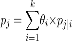(1)

There are n specimens. The probability of observing j strains in each is p_j, where j = 1, 2…k. Thus, by definition, the Y vector follows a multinomial distribution:

(2)

Denote the prior distribution by π(θ) (equation 3). The Dirichlet distribution is used because it provides a means of expressing quantities that vary randomly and independently of each other and yet obey the condition that their sum remains fixed. This provides a means for assigning prior sample size (weight) to the prior distribution statement (5):

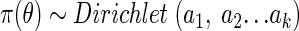(3)

Equations 1, 2, and 3 give the posterior distribution:

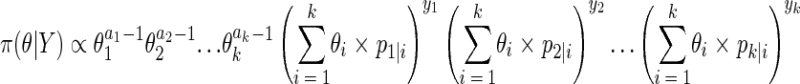(4)

The independent Metropolis-Hastings algorithm was used to simulate the posterior distribution given in equation 4 (4, 9). The simulation means were used to estimate [θ] and p was computed by 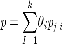, where p_j|i is calculated as shown in the next paragraph. Thus, the mean can be used to estimate the probability of observing all strains present in the sample according to sample size.

Computation of p_j|i. Recall that p_j|i is the probability of observing j strains given that the specimen contains i strains. Suppose there are i strains in a specimen; the equal concentrations assumption means that a randomly selected isolate has the same probability (1/i) of representing any one of the i strains. Suppose there are i strains, at most, in a specimen; take n isolates from this specimen. Let X = (x₁, x₂…x_i) denote the vector of counts, where x_k gives the number of isolates out of n that are from each strain k for k = 1, 2…i. From the equal concentrations assumption, the following equation is derived:

(5)

A simulation was performed using Visual Basic code (Microsoft Corporation, Seattle, Wash.) to enumerate the number of strains per specimen. For any given i, 1,000,000 X vectors were simulated using X ∼ multinomial (n; 1/i, 1/i…1/i). The numbers of X vectors containing 1, 2… in nonempty elements were counted. These counts were divided by 1,000,000 (the total number of simulations) and used to estimate p_j|i values.

REFERENCES

- 1.Altekruse, S., J. Koehler, F. Hickman-Brenner, R. V. Tauxe, and K. Ferris. 1993. A comparison of Salmonella enteritidis phage types from egg-associated outbreaks and implicated laying flocks. Epidemiol. Infect. 110:17-22. [DOI] [PMC free article] [PubMed] [Google Scholar]
- 2.Caldwell, D. J., B. M. Hargis, D. E. Corrier, J. D. Williams, L. Vidal, and J. R. DeLoach. 1994. Predictive value of multiple drag-swab sampling for the detection of Salmonella from occupied or vacant poultry houses. Avian Dis. 38:461-466. [PubMed] [Google Scholar]
- 3.Ewing, W. H. 1986. Edwards and Ewing's identification of enterobacteriaceae, 4th ed. Elsevier Science Publishing Co. Inc., New York, N.Y.
- 4.Gelfand, A. E., and A. F. M. Smith. 1990. Sampling based approaches to calculating marginal densities. J. Am. Statist. Assoc. 85:398-409. [Google Scholar]
- 5.Johnson, N. L., and S. Kotz. 1972. Continuous multivariate distributions, p. 231-235. Wiley, New York, N.Y.
- 6.Kramer, J. M., J. A. Frost, F. J. Bolton, and D. R. Wareing. 2000. Campylobacter contamination of raw meat and poultry at retail sale: identification of multiple types and comparison with isolates from human infection. J. Food Prot. 63:1654-1659. [DOI] [PubMed] [Google Scholar]
- 7.Kumar, M. C., H. R. Olson, L. T. Ausherman, W. B. Thurber, M. Field, W. H. Hohlstein, and B. S. Pomeroy. 1972. Evaluation of monitoring programs for Salmonella infection in turkey breeding flocks. Avian Dis. 16:644-648. [PubMed] [Google Scholar]
- 8.Singer, R. S., W. O. Johnson, J. S. Jeffrey, R. P. Chin, T. E. Carpenter, E. R. Atwill, and D. C. Hirsh. 2000. A statistical model for assessing sample size for bacterial colony selection: a case study of Escherichia coli and avian cellulitis. J. Vet. Diagn. Investig. 12:118-125. [DOI] [PubMed] [Google Scholar]
- 9.Tierney, L. 1994. Markov chains for exploring posterior distributions. Ann. Stat. 22:1701-1762. [Google Scholar]
- 10.U.S. Food and Drug Administration. 1998. Bacteriological analytical manual, 8th ed. U.S. Food and Drug Administration, Washington, D.C.
- 11.Ward, L. R., J. D. de Sa, and B. Rowe. 1987. A phage-typing scheme for Salmonella enteritidis. Epidemiol. Infect. 99:291-294. [DOI] [PMC free article] [PubMed] [Google Scholar]
- 12.Wassenaar, T. M., and D. G. Newell. 2000. Genotyping of Campylobacter spp. Appl. Environ. Microbiol. 66:1-9. [DOI] [PMC free article] [PubMed] [Google Scholar]