Modified Regression Model for the Logan Plot

Summary

Logan's graphical model is a robust estimation of the total distribution volume (DVt) of reversibly bound radio-pharmaceuticals, but the resulting DVt values decrease with increasing noise. The authors hypothesized that the noise dependence can be reduced by a linear regression model that minimizes the sum of squared perpendicular rather than vertical (y) distances between the data points and fitted straight line. To test the new method, 15 levels of simulated noise (repeated 2,000 times) were added to synthetic tissue activity curves, calculated from two different sets of kinetic parameters. Contrary to the traditional method, there was no (P > 0.05) or dramatically decreased noise dependence with the perpendicular model. Real dynamic ¹¹C (+) McN5652 serotonin transporter binding data were processed either by applying Logan analysis to average counts of large areas or by averaging the Logan slopes of individual-voxel data. There were no significant differences between the parameters when the perpendicular regression method was used with both approaches. The presented experiments show that the DVt calculated from the Logan plot is much less noise dependent if the linear regression model accounts for errors in both the x and y variables, allowing fast creation of unbiased parametric images from dynamic positron-emission tomography studies.

There are two approaches to the quantitative analysis of binding data obtained from dynamic imaging of γ or positron-emitting radionuclides. The first approach uses compartmental models, and is usually referred to as kinetic analysis (Carson, 1996). The second approach involves the application of a suitable transformation to the data so that the correspondence between two variables becomes linear over a time interval, and is called graphical analysis (Logan, 2000). The two most frequently applied graphical methods are the Patlak plot (Patlak et al., 1983) for irreversible binding, and the Logan plot (Logan et al., 1990) for reversible binding (Logan, 2000). With both graphical methods, the slope of the transformed graph is used for quantification of radioligand binding.

Although graphical methods are easier to perform and are generally considered more robust for noisy data sets, it has been shown using simulated data that the slope obtained from the Logan plot with the traditional linear regression model is biased, resulting in increasing underestimation of distribution volumes with increasing noise (Abi-Dargham et al., 2000; Slifstein and Laruelle, 2000; Logan et al., 2001). Some articles point out that a possible reason for the bias is that the errors add up during integration; to compensate for this effect, the application of nonlinear or generalized linear iterative least-squares methods have been proposed (Feng et al., 1993, 1996; Logan et al., 2001).

We hypothesized that the traditional linear regression model is basically unsuitable for graphical analysis because it only takes into account the errors in the Y variable. The aim of the present work was to test whether the bias in the Logan slope can be diminished by using a modified noniterative linear regression model that accounts for errors in both variables.

MATERIALS AND METHODS

Linear regression models

Traditional linear regression.

With the original linear regression model, referred to here as traditional, the measured (noisy) values y_i are plotted against an independent variable x with negligible error. Estimates of the regression parameters

$$y=m\cdot x+b$$

are searched for by minimizing the sum of squared differences between the measured (y_i) and estimated (ŷ_i) values, in the simplest case without weighting:

$$s_c=\sum _{i=1}^n\Delta {y_i}^2=\sum _{i=1}^n{(y_i-{\widehat{y}}_i)}^2$$

The minimal value of s_c is reached when the regression parameters are

$$m=Q_{xy}∕Q_{xx},b=\stackrel{‒}{y}-m\cdot \stackrel{‒}{x}$$

with x̄ and ȳ being the averages of x_i and y_i values, respectively, and

$$Q_{xx}=\sum _i{(x_i-\stackrel{‒}{x})}^2,Q_{xy}=\sum _i(x_i-\stackrel{‒}{x})\cdot (y_i-\stackrel{‒}{y})$$

Perpendicular linear regression model.

When both the x and y variables are subject to measurement errors, a more advanced line fitting method has been developed, based on the minimization of the sum of squared distances between the measured points and the fitted straight line:

$$s_p=\sum _{i=1}^n{d_i}^2$$

Note that the general definition of d_i may take into account both the relative magnitude and the (point-by-point) relative error of the variables x and y, allowing an arbitrary angle of the line section going through (x_i, y_i) and the fitted line. For the present study, simply the Euclidean (perpendicular) distance was used (Fig. 1), and the regression parameters could be calculated from the equations:

$$\begin{array}{cc}\hfill 0=& {m_p}^2\cdot Q_{xy}+m_p\cdot (Q_{xx}-Q_{yy})-Q_{xy}\hfill \\ \hfill b_p=& \stackrel{‒}{y}-m_p\cdot \stackrel{‒}{x}\hfill \end{array}$$

FIG. 1.

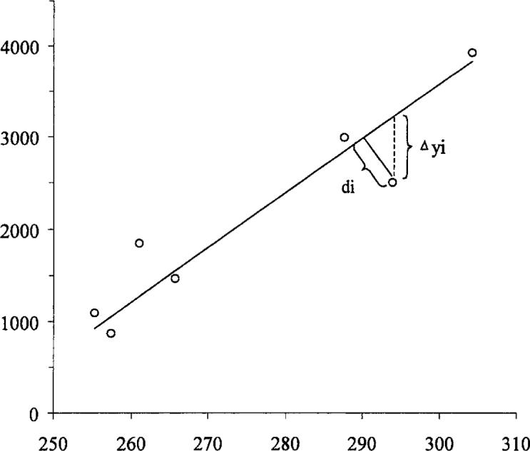
Difference between the traditional and perpendicular line-fitting models. Δy_i is the difference between the measured and the estimated y value; d_i is the distance between the point and the line.

with the coefficients defined in the previous section.

Logan plot

The Logan plot is described by the equation (Logan et al., 1990)

$$\frac{{\int }_0^t{C}_{tissue}\left(u\right)du}{C_{tissue}\left(t\right)}=DVt.\frac{{\int }_0^t{C}_{plasma}\left(u\right)du}{C_{tissue}\left(t\right)}+V$$

where C_tissue and C_plasma are radiotracer concentrations in the tissue region and in the plasma, respectively. The slope of the fitted straight line represents the so-called total distribution volume (DVt) (Logan, 2000).

Test data sets with simulated noise

Two sets of synthetic data and a real tissue time–activity curve were used for noise simulation studies. An arterial activity input function was obtained by fitting the sum of three exponentials to the logarithm of a typical arterial time–concentration curve (Fig. 2A) (Abi-Dargham et al., 2000). Simulated Gaussian error was added to the tissue curves (Logan et al., 2001), the details of which are listed in the Appendix. The simulations were repeated 2,000 times. Both the traditional and the perpendicular linear regression models were applied to each individual noisy data set, and the averages and standard deviations of the slopes were calculated for each error level. The error level was characterized by the mean of the coefficients of variation (CV) at the last eight data points used for line fitting.

FIG. 2.

Input data for the calculations. (A) Arterial input curve. (B) Synthetic (synt.) and measured tissue curves. ID, injected dose.

Synthetic data set 1, with lower distribution volume.

To allow direct comparison with the results of Abi-Dargham et al. (2000), the parameters described in their report were used (K₁ = 0.13 mL·g^–1·min^–1, k₂ = 0.057/min, k₃ = 0.11/min, and k₄ = 0.034/min, for a theoretical DVt = 9.7 mL/mL. Simulated Gaussian error was added to the synthetic curve at 15 different error levels. The noise model used by Abi-Dargham et al. (2000) was not the same, as these investigators considered the effect of radioactivity decay only, but not imaging time or the changes in ligand concentration.

Synthetic data set 2, with higher distribution volume.

To allow comparison with the generalized linear iterative least-squares method, a synthetic “tissue” curve with the same parameters as used by Logan et al. (2001) was used ([¹¹C]-d-threo-methylphenidate, K₁ = 0.6 mL·min^–1·mL^–1, k₂ = 0.06/min, k₃ = 0.5/min, and k₄ = 0.2/min, for a theoretical DVt of 35 mL/mL). Simulated noise was added at 15 different error levels.

Measured data with simulated noise added.

For a third experiment, the arterial and midbrain time–activity curves obtained in a (¹¹C (+) McN5652) positron-emission tomography study of a control patient were used. Additional noise was added to the measured values at 12 different levels, as described for the synthetic data in the previous section. The aim of this experiment was to test the behavior of the parameter estimations for data that are not necessarily confined to a theoretic three-compartment model.

Comparison of voxel-by-voxel and regional data.

The highest noise level is encountered when time–activity curves are generated on a voxel-by-voxel basis. To test whether the Logan slopes generated from single-voxel time–activity curves are biased when compared with the parameter of a larger volume, Logan analysis with the perpendicular regression model was applied to real data of a dynamic serotonin transporter (¹¹C (+) McN5652) positron-emission tomography study obtained in a patient with Parkinson disease. In the first approach, time–activity curves of large brain regions were generated and their Logan plot was obtained. In the second approach, the Logan slope was calculated from each voxel and the values were averaged over the same regions.

RESULTS

The averages and standard deviations of the Logan slope values calculated from the 2,000 simulations of the synthetic data set 1 at each noise level are shown in Fig. 3, for both regression models. With the traditional model, increasing noise resulted in decreasing slope values (negative bias). The perpendicular regression model resulted in fairly constant slope values, independent of the noise level (t-test: P > 0.05), though the SD of the slope values increased with the noise.

FIG. 3.

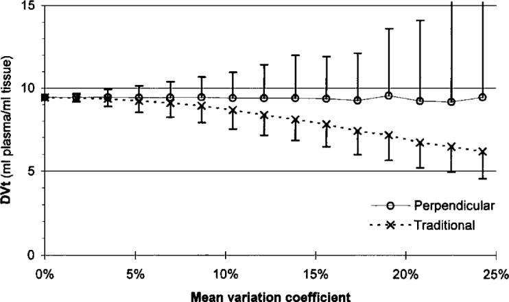
Dependence of the Logan slope (total distribution volume, DVt) on the added noise for synthetic data set 1.

Results for the simulations described for synthetic data set 2 are shown in Fig. 4. Although the random calculation error increased with noise, the average of the DVt values calculated by the perpendicular regression model showed only 3% decrease between 0% and 25% added noise.

FIG. 4.

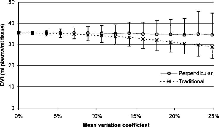
Dependence of the Logan slope (total distribution volume, DVt) on the added noise for synthetic data set 2.

Figure 5 shows the result when noise was added to a real measured time–activity curve. Because the baseline curves contained noise, the two regression models gave different slope averages, even when no noise was added. The perpendicular model resulted in a fairly constant DVt to 7% CV of the added noise, and increased only slightly at higher noise levels.

FIG. 5.

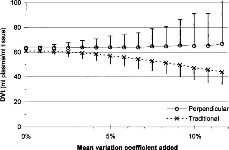
Dependence of the Logan slope (total distribution volume, DVt) on the noise added to a measured tissue time–activity curve.

Figure 6 shows the rates of change (average percent difference from a noiseless estimate of the DVt over 1% increase in the CV of noise), and shows a dramatic decrease in the bias when applying the perpendicular rather than the traditional method.

FIG. 6.

Comparison of the magnitudes of relative change rate, defined as the average bias introduced by increasing the coefficient of variation (CV) of the noise by 1%.

The DVt estimations with the traditional method were significantly lower than with the perpendicular method at all nonzero CV levels in all the three simulation experiments (Welch d-test with Bonferroni correction for multiple comparisons; P < 0.01 at CV=1.7% in synthetic data set 1, P < 0.001 in all other cases).

Table 1 presents Logan slope values calculated from the average curves of various brain regions compared with the averages of the values in the Logan parametric images over the same regions. Both regression models were applied. Regions of low (cerebellum, parietal) and high (putamen, caudate) total distribution volumes are included. Although there were no significant differences with the perpendicular model, the voxel-by-voxel calculations gave significantly lower values with the traditional model (paired t-test, P < 0.05). The calculation time of the Logan parametric images (using a C++ Windows-based program) was 0.5 s/slice for a typical dynamic brain positron-emission tomography study (18 frames, 128×128 pixel matrix). Examples for single pixel Logan plots are shown in Fig. 7.

TABLE 1.

Comparison of the Logan slopes, calculated either from time–activity curves of large regions, or on a voxel-by-voxel basis

	Perpendicular		Traditional
Region	Curves	Voxels	Curves	Voxels
Cerebellum	29.1	29.5	29.1	28.8
R. caudate	51.3	51.4	51.3	41.1
R. putamen	53.3	51.7	53.2	47.6
R. pariet	29.1	29.0	29.1	27.2

Values are in mL plasma/mL tissue units. Both regression models gave the same result when applied to large regions. The voxel-by-voxel calculation with the traditional model underestimated the distribution volumes; higher values were more seriously biased. The perpendicular model, in contrast, gave practically the same mean voxel-by-voxel and regional values.

FIG. 7.

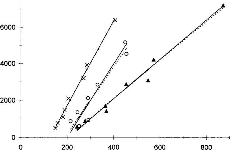
Sample Logan plots from single-pixel regions of a brainreceptor positron-emission tomography study. Continuous lines were calculated using the perpendicular, whereas dotted lines were calculated using the traditional linear regression model.

DISCUSSION

Graphical methods present an attractive alternative to compartmental analysis of radionuclide studies because of their robustness and simplicity, making them suitable for calculating parametric images. Logan analysis is the graphical method applicable to reversibly bound tracers. However, recent papers (Slifstein and Laruelle, 2000; Abi-Dargham et al., 2000) have been rather discouraging. Using data from simulation experiments, they concluded that the Logan slope was seriously biased, and was therefore not dependable when significant noise was present in the data. It has also been described that the bias increases with increasing DVt. Smaller (positive) bias was observed when the generalized linear least-squares method was used (Logan et al., 2001).

Our hypothesis that the calculation method of linear regression parameters may influence the presence of bias in the resulting Logan slope was proven by the simulation data presented. When applying even the simplest (unweighted) regression model that accounts for errors in both variables, the expected value of the Logan slope became almost independent of the amount of noise usually found in real clinical measurements. In contrast to the solutions suggested previously (Feng et al., 1993, 1996; Logan et al., 2001), our method is single step rather than iterative. With the proposed perpendicular regression model, Logan parametric images resulted in the same regional average values as those gained from pooled (less noisy) time–activity curves. A similar adjustment of the error model is not necessary for kinetic analysis because in that case the error in the time (x) variable is negligible.

In conclusion, using a perpendicular linear regression model to calculate the total distribution volume from the Logan plot can substantially reduce the bias usually encountered with the traditional procedure. The proposed single-step method allows for fast generation of parametric images.

Appendix: Noise model

Let y be the ligand concentration in the region of interest, and c the counts measured in Δt image duration at time t. Then

$$c=\frac{y\cdot d\cdot \Delta t}{a}$$ (Eq. A1)

with scaling factor a, and the decay factor d for radionuclide half time T being

$$d={0.5}^{t∕T}$$

Because of the error of the measured counts

$$\Delta c=\sqrt{c}$$

and from Eq. A1, the error of the concentration y is

$$\Delta y=\frac{a\cdot \Delta c}{d\cdot \Delta t}$$

We can express the coefficient of variation CV as

$$CV=\frac{\Delta y}{y}=\sqrt{\frac{a}{y\cdot d\cdot \Delta t}}$$

Hence, the noisy data are calculated as

$$\tilde{y}=y\cdot [1+CV\cdot G(0,1)]$$

with G (0,1) being a randomly generated number of Gaussian distribution (mean 0, SD 1).

Apart from notational differences, this error model is equivalent to the one used by Logan et al. (2001).

REFERENCES

- Abi-Dargham A, Martinez D, Mawlawi O, Simpson N, Hwang DR, Slifstein M, Anjilvel S, Pidcock J, Guo NN, Lombardo I, Mann JJ, Van Heertum R, Foged C, Halldin C, Laruelle M. Measurement of striatal and extrastriatal dopamine D1 receptor binding potential with [11C]NNC 112 in humans: validation and reproducibility. J Cereb Blood Flow Metab. 2000;20:225–243. doi: 10.1097/00004647-200002000-00003. [DOI] [PubMed] [Google Scholar]
- Carson RE. Mathematical modeling and compartmental analysis. In: Harbert JC, Eckelman WC, Neumann RD, editors. Nuclear medicine diagnosis and therapy. Thieme Medical Publishers; New York, NY: 1996. pp. 167–193. [Google Scholar]
- Feng D, Wang Z, Huang SC. A study on statistically reliable and computationally efficient algorithms for generating local cerebral blood flow parametric images with positron emission tomography. IEEE Trans Biomed Eng. 1993;12:182–188. doi: 10.1109/42.232247. [DOI] [PubMed] [Google Scholar]
- Feng D, Huang SC, Wang Z, Ho D. An unbiased parametric imaging algorithm for nonuniformly sampled biomedical system parameter estimation. IEEE Trans Biomed Eng. 1996;15:512–518. doi: 10.1109/42.511754. [DOI] [PubMed] [Google Scholar]
- Logan J. Graphical analysis of PET data applied to reversible and irreversible tracers. Nucl Med Biol. 2000;27:661–670. doi: 10.1016/s0969-8051(00)00137-2. [DOI] [PubMed] [Google Scholar]
- Logan J, Fowler JS, Volkow ND, Wolf AP, Dewey SL, Schlyer DJ, MacGregor RR, Hitzemann R, Bendriem B, Gatley SJ. Graphical analysis of reversible radioligand binding from time-activity measurements applied to [N-11C-methyl]-(-)-cocaine PET studies in human subjects. J Cereb Blood Flow Metab. 1990;10:740–747. doi: 10.1038/jcbfm.1990.127. [DOI] [PubMed] [Google Scholar]
- Logan J, Fowler JS, Volkow ND, Ding YS, Wang GJ, Alexoff DL. A strategy for removing the bias in the graphical analysis method. J Cereb Blood Flow Metab. 2001;21:307–320. doi: 10.1097/00004647-200103000-00014. [DOI] [PubMed] [Google Scholar]
- Patlak CS, Blasberg RG, Fenstermacher JD. Graphical evaluation of blood-to-brain transfer constants from multiple-time uptake data. J Cereb Blood Flow Metab. 1983;3:1–7. doi: 10.1038/jcbfm.1983.1. [DOI] [PubMed] [Google Scholar]
- Slifstein M, Laruelle M. Effects of statistical noise on graphic analysis of PET neuroreceptor studies. J Nucl Med. 2000;41:2083–2088. [PubMed] [Google Scholar]