Volumetric Neuroimage Analysis Extensions for the MIPAV Software Package

Abstract

We describe a new collection of publicly available software tools for performing quantitative neuroimage analysis. The tools perform semi-automatic brain extraction, tissue classification, Talairach alignment, and atlas-based measurements within a user-friendly graphical environment. They are implemented as plug-ins for MIPAV, a freely available medical image processing software package from the National Institutes of Health. Because the plug-ins and MIPAV are implemented in Java, both can be utilized on nearly any operating system platform. In addition to the software plug-ins, we have also released a digital version of the Talairach atlas that can be used to perform regional volumetric analyses. Several studies are conducted applying the new tools to simulated and real neuroimaging data sets.

1 Introduction

Segmentation of structural magnetic resonance (MR) brain images is a critical step in many neuroscientific applications such as in the morphological analyses of different diseases, characterization of the relationship between brain structure and function, and in treatment monitoring and planning (Pham et al. (2000)). Most publicly available software tools for performing segmentation tasks, however, are hindered by the lack of cross-platform compatibility, limited support of file formats, complex user interfaces, and an inability to manually edit the results. As a result, it is not uncommon for a segmentation analysis to require several different software packages for performing file conversion, image processing, manual editing, and volumetric measurements.

We have developed three software tools that cover some of the most common needs of quantitative neuroimage analysis: 1) brain extraction - isolation of the brain region and removal of external structures, 2) tissue classification - identification of the gray matter, white matter, and cerebrospinal fluid (CSF) tissues, and 3) Talairach alignment - alignment to a standardized coordinate system and quantification using digital atlases. The methods upon which the tools are based have been previously published and validated but until now, have not been available in an integrated, user-friendly, and cross-platform software package.

All of the software tools have been implemented as plug-ins for the Medical Image Processing, Analysis, and Visualization (MIPAV) software package developed at the Center for Information Technology, National Institutes of Health (McAuliffe et al. (2001)). MIPAV enables quantitative analysis and visualization of medical images from multiple modalities such as PET, MRI, CT, and microscopy. It includes basic and advanced computational methods to analyze and quantify biomedical data, supports all major medical image formats, and provides many visualization and data manipulation tools for 2D and 3D images or image series. Because MIPAV is Java-based, it can be utilized on nearly any operating system, such as Windows, Linux, and MacOS. MIPAV also provides an intuitive graphical user interface, providing researchers a user-friendly tool to visualize and analyze their imaging data. The entire software package and documentation may be downloaded from the internet (http://mipav.cit.nih.gov).

When applied in conjunction with our provided digital atlas, our tools can be used for performing regional volumetric analyses. This approach is loosely based on the approach of Andreasen et al. (1996). In their work, the unlabeled brain image is first placed into Talairach space using a standard piecewise affine transformation. Selected labels from the Talairach-Tournoux brain atlas (Talairach and Tournoux (1988)) are then superimposed on the transformed brain, and the volume of brain tissues inside each of the labeled regions is measured. It was shown that these measurements provide accurate volumetrics of gross anatomical brain structures, such as lobes, and the procedure is very fast. In our version of the method, the studied brain image may be first segmented into gray matter, white matter, and CSF, and this segmentation is then transferred into Talairach coordinates. Labels of the regions of interest are selected and transferred to the image, and the volume of tissues included in each region may be computed separately for each tissue. Before quantification, the labels may also be manually refined using the various editing tools already incorporated into MIPAV.

In this paper, we describe the software tools, as well as our Talairach digital atlas, and show how these tools can be used for performing regional volumetric analysis. We have made both the software tools and atlas data available on the internet (http://medic.rad.jhu.edu). Discussion forums are also provided on the same website for technical support and a detailed tutorial on the usage of these tools is available as a technical guide.

2 Methods

2.1 The MIPAV Software Package

To support the National Institutes of Health (NIH) intramural research program, the Biomedical Research and Services Section (BIRSS) has developed MIPAV, a multifaceted, platform-independent, quantification, and visualization application for biomedical images. MIPAV is a Java-enabled application that encompasses the functionality to process, quantify and visualize data sets from micro (eg. crystallography, microscopy) to macro (eg. CT, MRI). MIPAV supports numerous medical and research file formats including Zeiss, Biorad, TIFF, DICOM 3.0, NIFTI, AFNI, MINC, GE, Siemens, Philips, AVI, Interfile, MIPAV XML, and new formats are added as needed. Figure 1 shows the graphical user interface and some of the visualization and manual editing capabilities offered by MIPAV.

Fig. 1.

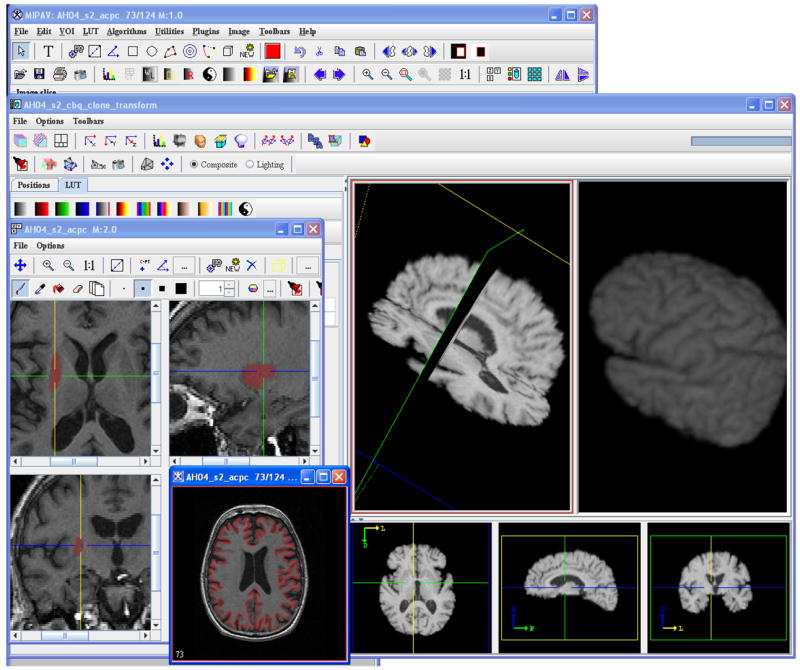
The MIPAV graphical user interface. Painting in a tri-planar view, volume rendering, and contour-based segmentation tools are a few of the capabilities offered by the software package.

From a system perspective, MIPAV was designed to support multiple levels of user needs: core, scripts, and plug-ins. Core functionality addresses basic user needs including comprehensive VOI support, manual annotation and delineation, reading/writing all supported file formats, and various image processing, filtering, segmentation, and registration algorithms. Core visualization tools include tri-planar visualization and editing, image and movie capture, 3D surface and volume rendering, and 2D/3D fusion of multichannel datasets. In addition, MIPAV interfaces with the Insight Segmentation and Registration Toolkit (ITK) (Ibanez and Schroeder (2005)). To facilitate repetitive processing, MIPAV incorporates scripting abilities and supports command line execution. The scripting mechanism may be used to record a sequence of image processing and analysis operations and then apply the recorded operations to a series of datasets. User specific needs can be met by developing plug-ins using MIPAV’s open application programming interface.

The software tools described in this paper were developed as Java plug-ins for MI-PAV. During initialization, MIPAV automatically loads installed plug-ins and builds the plug-in menu, allowing them to be utilized as if they were native algorithms. The plug-ins that do not directly require user interaction (eg. tissue classification) may also be used with MIPAV’s scripting interface, thereby facilitating batch processing.

2.2 The Brainstrip Tool

It is often desirable to remove unwanted structures from MR brain images as a preliminary step prior to volumetric analyses. These structures include regions corresponding to the skull, eyes, skin, and dura. This step is unfortunately difficult, typically requiring several hours to manually segment the brain tissue, depending on the desired quality for the result. As an alternative to manual segmentation, fully automated techniques are available (Smith (2002); Shattuck and Leahy (2002); Segonne et al. (2004); Rex et al. (2004); Rehm et al. (2004)), but these methods still benefit from subsequent editing (Fennema-Notestine et al. (2006)).

We have implemented a semiautomatic approach that substantially reduces manual processing times and is based on the method employed and validated by Goldszal et al. (1998). The philosophy of this approach is to interactively obtain a reasonable estimate of the brain mask that can be refined manually. Given some simple input information from the user (the minimum and maximum intensity of the gray and white matter, a seed point defined inside the brain, and a bounding box for the brain), a sequence of automatic processing routines extract an approximate brain volume. The first step in the sequence thresholds the image based on the provided intensity values. A morphological erosion using a spherical structuring element (typically set to 5mm) is then applied to the thresholded volume to remove any bridges that occur between the brain tissue and dura. Next, the provided seed point is used to perform a region growing algorithm to extract the central portion of the brain volume. Two dilations with the same structuring element are then applied to recover the lost tissue and smooth the overall surface. Finally, holes within the mask are removed by performing a 2-D region growing on each slice within the background and retaining the complement. Optionally, a three-dimensional bounding box input may be defined by the user to decide where to cut the brainstem, or select a region of the brain. Fig. 2 shows the actual brainstrip user interface. The extracted region is superimposed on the original image and can then be manually edited to attain the accuracy of fully manual methods.

Fig. 2.

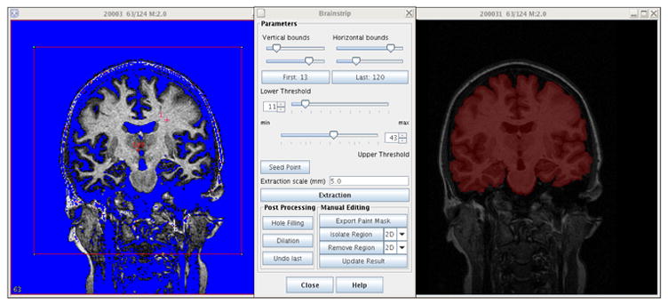
The skull stripping plug-in: original image, interface, and stripped image mask overlaid on original image (from left to right).

Selection of the inputs will typically require less than one minute for a trained operator. The output result is generated within a few seconds on a typical PC after the inputs have been provided. Because the method is simple and fast, the operator has the ability to quickly and easily make adjustments should the initial input parameters yield a poor result. Because all aspects of the processing are provided through MIPAV, the need to switch to separate software programs for performing any manual refinement is eliminated. Note also that MIPAV natively provides its own implementation of two popular algorithms for fully automatic brain stripping: Brain Surface Extractor (BSE) (Shattuck and Leahy (2002)) and Brain Extraction Tool (BET) (Smith (2002)).

2.3 The FANTASM Tool

Tissue classification algorithms typically segment the brain into its three major tissue types: gray matter, white matter, and CSF. Many algorithms have been proposed in the literature that perform tissue classification in the presence of MR imaging artifacts, such as noise and intensity inhomogeneities (Wells et al. (1996); Leemput et al. (1999); Pham and Prince (1999); Shattuck et al. (2001); Smith (2002). Our tool is based on the Fuzzy And Noise Tolerant Adaptive Segmentation Method (FANTASM) (Pham (2001a); Han et al. (2004)). Given the number of tissue classes, the technique automatically classifies each pixel of the image as one of the tissues, estimates the inhomogeneity field, and also attributes a membership value from 0 to 1 for each class.

We briefly describe FANTASM in the following. Our implementation in this work differs slightly from the implementation described in Han et al. (2004) in that we explicitly model the gain field parametrically as a polynomial field. Let Ω be the set of voxel indices, C be the number of tissue classes, and y_j, j ∈ Ω be the observed (preprocessed) MR image values, which may be a vector in the case of multichannel images. The goal of FANTASM is to find intensity centroids v_k, k = 1, . . . , C, a gain field g_j, j ∈ Ω, and membership values u_jk, j ∈ Ω, k = 1, . . . , C that will minimize the following objective function:

$$J_{\text{FANTASM}}=\sum _{j\in \mathrm{\Omega }}\sum _{k=1}^C{u}_{jk}^q\parallel {\mathbf{y}}_j-g_j{\mathbf{v}}_k{\parallel }^2+\frac{\beta }{2}\sum _{j\in \mathrm{\Omega }}\sum _{k=1}^C{u}_{jk}^q\sum _{l\in N_j}\sum _{m\ne k}{u}_{lm}^q$$ (1)

Note that the membership values are constrained to be greater than zero and satisfy ${\sum }_{k=1}^C{u}_{jk}=1$.

The first term in (1) is simply the fuzzy c-means clustering objective function (Bezdek et al. (1993)) with a gain field term that allows the centroids to spatially vary throughout the image. The parameter q, which must satisfy q > 1 (and is set to 2 in this work), determines the amount of “fuzziness” of the resulting classification (Bezdek et al. (1993)). The parameter C is the number of classes and is assumed to be known. For brain images, this typically is set equal to 3, corresponding to gray matter, white matter, and CSF. The second term in (1) is a penalty function that forces the tissue memberships to be smooth, where the parameter β is a weight that determines the amount of smoothness (Pham (2001b)). In practice, we use a normalized smoothness parameter that is multiplied by the square of the intensity range of the image. The symbol N_j represents the set of first order neighbors of pixel j.

We make the simplifying assumption that the gain field g can be represented by a low-degree three-dimensional polynomial function. Although this assumption is somewhat more restrictive than that of Han et al. (2004), it is usually sufficient to model the intensity variations (cf. Leemput et al. (1999)), is computationally more efficient, and requires fewer parameters to be specified. Mathematically, this can be expressed as:

$$g_j=\sum _{n=1}^N{f}_n{P}_n(j)$$

where P_n are polynomial basis functions and f_n are the coefficients. We use Chebyshev polynomial basis functions for their numerical stability and other advantageous properties for function approximation (Davis (1975)). The number of Chebyshev coefficients are 20 for the 3rd degree case, and 35 for 4th degree polynomial fields. Because the gain field is assumed to be smooth and the equations are overdetermined, we subsample the images by a factor of 3 along each dimension when computing the coefficients f_n to increase the computational efficiency.

An iterative algorithm for minimizing (1) can be derived by solving for a zero gradient condition with respect to the memberships and the centroids and can be described as follows:

Algorithm: Polynomial gain field FANTASM

1. Obtain initial estimates of the centroids, v_k.

2. Compute membership functions:

   $$u_{jk}=\frac{{\left(\parallel {\mathbf{y}}_j-g_j{\mathbf{v}}_k{\parallel }^2+\beta \sum _{l\in N_j}\sum _{m\ne k}{u}_{lm}^q\right)}^{-1/(q-1)}}{\sum _{i=1}^C{\left(\parallel {\mathbf{y}}_j-g_j{\mathbf{v}}_i{\parallel }^2+\beta \sum _{l\in N_j}\sum _{m\ne i}{u}_{lm}^q\right)}^{-1/(q-1)}}.$$ (2)
3. Compute centroids:

   $${\mathbf{v}}_k=\frac{\sum _{j\in \mathrm{\Omega }}{u}_{jk}^q{g}_j{\mathbf{y}}_j}{\sum _{j\in \mathrm{\Omega }}{u}_{jk}^q{g}_j^2},\hspace{0.17em}k=1,\dots ,C.$$ (3)
4. Compute gain field by solving the following matrix equation for the coefficients f_n:

   $$[u_{jk}{\mathbf{v}}_k{P}_n(j)]·[f_n]=[u_{jk}{\mathbf{y}}_j].$$ (4)

5. Go to Step 2 and repeat until convergence.

We assume that the algorithm has converged when the maximum change in membership values between iterations is less than 0.01. In order to decrease the possibility of convergence to a local minimum, the degree of the polynomial gain field is initially set to zero and then eventually increased to the desired value as convergence is achieved. Fig. 3 shows the actual FANTASM plug-in user interface. The additional tabs allow specification of multichannel data sets and various algorithm parameters.

Fig. 3.

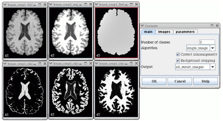
The tissue classification plug-in (clockwise from top left): the original image, classified image, inhomogeneity field, dialog box, white matter membership, gray matter membership, CSF membership.

2.4 The Talairach Tool

To draw comparisons between brains belonging to different subjects, it is often beneficial to define a common coordinate system. The brain atlas and coordinate system defined by Talairach and Tournoux (1988) is a commonly accepted standard in the neuroscientific community. The classical Talairach normalization procedure can be described as follows: 1) align the anterior and posterior commissures (AC and PC, respectively), and 2) scale the brain to align its boundaries to those of the atlas.

Although the transformation utilized in the Talairach transformation is relatively low-dimensional, particularly when compared to the more recently developed nonlinear deformation methods (Maintz and Viergever (1998); Christensen et al. (1997); Shen and Davatzikos (2002)), it is computationally fast and easy to control. For example, if after alignment the mid-sagittal plane is not vertical within the axial view or if the gross atlas labels deviate substantially from the underlying image, one can easily update the input parameters to correct the results. It is clear that a Talairach alignment will be of limited use for small sub-structures of the brain, but it has been shown to accurately and reliably align some larger regions, such as lobes (Andreasen et al. (1996)). In the following, we briefly describe the operation of our Talairach tool.

The first alignment within the Talairach transformation, often referred to as ’AC-PC alignment’, is a rigid-body Euclidean transformation (i.e. 3-D rotation and translation). It aligns the AC-PC coordinate systems of brains defined by their origins and axes. We therefore require a minimum of three points for AC-PC alignment: the AC, PC, and a mid-sagittal point (SG). With them, the entire new coordinate system is known, and the brain image can be transformed into this new space.

Our AC-PC alignment follows the same procedure as the AFNI software (Cox (1996)). While three point landmarks are required in theory, there can be problems when the AC or PC are larger than one voxel, or when the mid-sagittal plane is oblique with respect to the voxel grid. The AFNI method requires the operator to pick several additional landmarks, such as the limits of AC and PC, and points for accurately finding the mid-sagittal plane. It uses five point landmarks:

1. the AC superior edge: the top limit of the anterior commissure,

2. the AC posterior margin: the rear limit of the anterior commissure,

3. the PC inferior edge: the bottom limit of the posterior commissure,

4. a first mid-sagittal point (SG1) : any point in the mid-sagittal (inter-hemispheric) plane, above the corpus callosum,

5. a second mid-sagittal point (SG2): another point, if possible away from the first, of the mid-sagittal plane.

Finding these landmarks may require some training and familiarization with neuroanatomy. Once all landmarks are determined, it is straightforward to compute a rigid-body transformation such that the conditions of the AC-PC coordinate system are satisfied (Bazin et al. (2005)).

The second part of the Talairach alignment consists of scaling the brain to match its boundaries with those of the atlas. It is a 12 degrees-of-freedom, piecewise linear transform that brings the AC, PC, and anterior, posterior, left, right, inferior, and superior boundaries of the brain to normalized positions. To perform the Talairach scaling, the 6 extremal points (most anterior, posterior, left, right, inferior, and superior points), or alternatively the bounding box enclosing the brain, must be determined. Along with the AC and PC points, these landmarks define a set of 12 boxes. In each box, the image is independently scaled along the three dimensions to fit the normalized dimensions of the Talairach coordinates. Continuity is guaranteed as the boxes share common faces. Our tool can save and reload the transform information (position of AC, PC, AC-PC orientation and scale, and cortex boundaries) in a readable text file. This allows the transformation to be applied to additional co-registered images (eg. functional MR images, the output of tissue classification algorithms).

Figure 4 shows the user interface for performing the Talairach transformation. The user can select the various landmark points, compute the transformation, save the transformation, as well as compute the inverse transformation. This latter functionality can be used for transforming labels from a normalized template into the subject space.

Fig. 4.

The Talairach alignment plug-in: (clockwise from top left) main dialog box, original image, AC-PC aligned image, image after full Talairach transformation, triplanar view for AC-PC alignment landmark selection, AC-PC alignment dialog box.

2.5 Atlas Labels

Two general purpose brain atlases that have become popular due to their availability are the Talairach atlas (Talairach and Tournoux (1988); Lancaster et al. (2000); Nowinski and Belov (2003)) and the MNI/ICBM atlas ( Holmes et al. (1998)). Although the Talairach atlas (also known as the Talairach-Tournoux atlas) is the actual atlas from which the Talairach alignment procedure was created (Talairach and Tournoux (1988)), the atlas and the coordinate system are two separate entities. Other atlases, such as the ICBM atlas, can also be used within the coordinate system.

The Talairach atlas consists of 27 histological slices in the axial orientation on which many different structures have been manually delineated. In our atlas, we have included labeled regions for use in MIPAV, as well as a set of volumetric label images that can be used in any other imaging software. The atlas is based on manually corrected labels obtained from the Talairach Daemon database and therefore possesses a hierarchy of structures of different scale, from left and right cerebrum to individual Brodmann areas (see Fig. 5). The spatial resolution of the atlas is 1mm x 1mm x 4mm. The groups and structures are listed in Lancaster et al. (2000) and Bazin et al. (2005). Once images are aligned into a common coordinate system, they may be labeled using the atlas, thereby providing an indication of the location, size, and shape of the particular structure of interest. Most small structures, such as those at the Brodmann level, will unlikely be accurate after Talairach alignment, but larger regions (eg. lobes, ventricles) are often reasonably delineated and can be further refined manually using the core tools provided within MIPAV. The MNI/ICBM atlas is also available in the MIPAV format for download from our website.

Fig. 5.

The Talairach atlas for MIPAV: (a) the volumetric images with the structure labels (b) the corresponding VOIs, over a Talairach aligned brain.

2.6 Volume measurements

Our combined tools may be used to obtain regional volumetric measurements in the brain. This can be accomplished using the following protocol:

Regional Volumetric Measurement Protocol

1. Brainstrip: the images of interest are pre-processed in order to isolate the brain tissues in the image.

2. FANTASM: the voxels of the original image are classified into white matter, gray matter, or CSF.

3. Talairach: the brain image is aligned within the Talairach coordinate system.

4. Atlas Labels: the volumes of interest (VOIs) for the study are loaded from the Talairach atlas onto the aligned brain.

5. Atlas inverse transform: the aligned brain with VOIs is transformed back into its original image space.

6. Volume measurements: the number of voxels within the studied tissue class is counted for each VOI, using MIPAV VOI analysis tools.

Because the Talairach alignment is non-linear, any direct measurement in this coordinate system is irrelevant; voxels have a different resolution in different boxes. For this reason, Step 4 is required to bring back any Talairach-aligned image into the original or the AC-PC aligned coordinates.

Between steps (5) and (6), the operator has the additional option to perform manual editing of the VOI boundaries. Statistics from VOIs (eg. volume, mean intensity) are easily generated within MIPAV, as shown in Figure 6. The volume of gray or white matter within each VOI may be computed, as well as the total brain volume. For gross lobar measurements, the provided Talairach labels are often sufficient for many applications. Even if further refinement is required, the labels will likely yield substantial time savings over completely manual delineation. A technical instruction guide is available from the MIPAV and plug-in websites that provides a detailed description of the entire procedure (McAuliffe (2005)).

Fig. 6.

Volume measurements using the Talairach parcellation and the MIPAV statistics generator.

3 Results

3.1 Brainstrip validation

The Brainstrip tool was validated on ten MR head scans against a previously validated manual protocol performed using an in-house developed software package called “Measure” (Barta et al. (1997)). Images were acquired from a GE Signa 1.5 Tesla MR scanner using a T1-weighted MPRAGE imaging protocol with a voxel size of 0.9375 × 0.9375 × 1.5mm. The images included in this analysis were from healthy adults, ages 50 and older, who are participants in an on-going longitudinal study of aging and cognition (Bassett et al. (2006)). Raters were instructed to set the lower threshold in the Brainstrip tool high enough such that the CSF in the lateral ventricles was removed but not so high that it resulted in the erosion of temporal lobes. The upper threshold was set as low as possible without removing any white matter tissue. The brain region was then manually edited using MIPAV’s integrated paint tools.

Figure 7 shows a comparison of the total brain volumes computed semi-automatically using our plug-in vs. the manual results using the Measure program. Brain volume was defined as total gray and white matter as computed using FANTASM. The mean total brain volume computed manually was 1212.40 cubic centimeters (cc) with a standard deviation (SD) of 120.73 and the mean volume computed using Brainstrip was 1188.17cc with a SD of 106.37. The mean error was −24.23cc with a 95% confidence interval of −47.97cc to −0.48cc, equating to less than 4% error. Although there appears to be a slight bias in the Brainstrip results toward lower volumes, the differences were not statistically significant under a paired T-test. The mean absolute percent error was 2.85% (SD=1.81). A Pearson correlation analysis yielded an R² of 0.93, indicating a high level of agreement between the two approaches. Processing times for brain extraction were reduced from 4 to 8 hours using manual editing to 30 minutes to 1 hour using the Brainstrip plug-in with manual postprocessing.

Fig. 7.

Plot of total brain volumes in cubic centimeters (cc) estimated using the semi-automated approach with our Brainstrip plug-in against the manual approach. The red line plots the result of a linear regression.

3.2 FANTASM validation

The original FANTASM implementation has been previously validated on simulated and real images (Pham (2001a); Pham and Prince (2004)). The MIPAV plug-in implementation differs from the original mainly with respect to the gain field estimation. In this section, we compare the results of applying the new implementation to FMRIB’s Automated Segmentation Tool (FAST), another freely available, cross-platform tissue classification software tool (Zhang et al. (2001)). The two methods are validated on the Brainweb phantom from the Montreal Neurological Institute (Collins et al. (1998)).

Table 1 shows the results of applying both FANTASM and FAST to the Brainweb phantom simulated with various noise levels (indicated by ‘N’), and inhomogeneity levels (indicated by ‘I’). The smoothness parameter setting for FANTASM was set at 0.3 for all images and a 3rd degree polynomial function was used to model the gain field. Different smoothness parameter settings were tested for FAST but because this value seemed to have little effect on the resulting performance, it was left at its default setting. From the results, it is apparent that FANTASM performed well at low noise levels and seemed to be very robust to inhomogeneity artifacts. FAST did not perform as well at low noise levels but was more robust to increases in noise.

Table 1.

Classification errors for FANTASM and FAST. “Mem” refers to membership values, “Pve” refers to partial volume estimates, and “Prob” refers to the posterior probability values.

Method	3%N, 0%I	3%N,20%I	3%N,40%I	5%N,20%I	7%N,20%I
FANTASM	4.36%	4.48%	4.51%	5.36%	6.49%
FAST	6.22%	6.39%	7.44%	6.30%	7.01%
FANTASM-Mem	0.055	0.056	0.056	0.066	0.078
FAST-Pve	0.086	0.085	0.089	0.091	0.097
FAST-Prob	0.070	0.070	0.075	0.067	0.069

The last three rows of Table 1 show the mean error between the true partial volume and the FANTASM membership functions, FAST partial volume estimates, and FAST posterior probability values, respectively. The FANTASM membership functions appear to better model the partial volume effects within the Brainweb image. The FAST partial volume estimates tended to provide an overly fuzzy representation relative to the true values while the posterior probabilities appeared to be too binarized. This is illustrated in Figure 8.

Fig. 8.

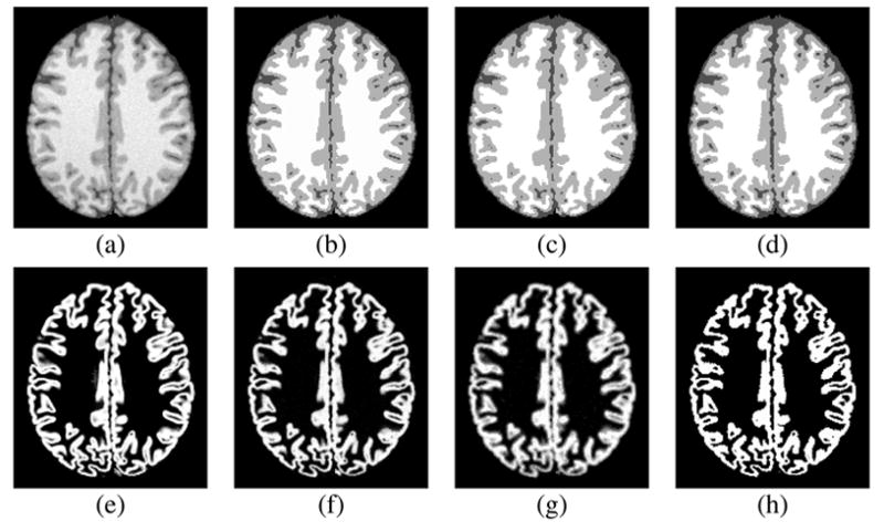
FANTASM and FAST applied to the Brainweb phantom: (a) phantom image with 3% noise and 20% inhomogeneity, (b) true classification, (c) FANTASM classification (d) FAST classification, (e) true gray matter partial volume, (f) FANTASM gray matter membership, (g) FAST gray matter partial volume, (h) FAST gray matter probability map.

FANTASM typically requires approximately four minutes of computation time to segment an MR image with 1mm cubic resolution on a typical PC workstation (3GHz Intel processor). In our tests, FAST required approximately 8 minutes on average. Although the Java programming language is sometimes criticized for slow execution times, in practice we have found negligible differences in speed when compared to equivalent C code during floating-point intensive operations.

3.3 Talairach validation

A sample of 20 scans from the same study described in Section 3.1 was used to evaluate the validity of frontal lobe measurements using the new tools. The images first were processed with the Brainstrip tool to isolate brain tissue. Left and right frontal lobes were manually segmented in the Measure software, according to a previously published methodology that has an inter-rater reliability of 0.99 (Aylward et al. (1997)). Figure 9 shows a typical result of manual vs. Talairach parcellation and Figure 10 shows plots of the resulting volumes for the frontal lobes in each hemisphere. The mean left frontal lobe volume was estimated to be 145.4cc (SD=30.7) using manual delineation. The mean volume of the same region computed using our Talairach tool was 146.2cc (SD=29.3). The mean right frontal lobe volume computed using the same two methods was 151.4cc (SD=34.1) and 154.9cc (SD=32.0), respectively. The intra-rater reliability between these methods was assessed using Intra-class correlation (ICC = 0.95 on the right, ICC = 0.97 on the left). A Pearson correlation model was also estimated with R² = 0.964 for the left and 0.975 for the right frontal lobe. This suggests that the Talairach-labeled volumes are good predictors of the actual volumes as determined by manual segmentation.

Fig. 9.

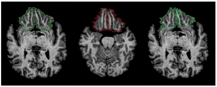
Frontal lobe delineations performed manually (left), using Talairach labels (center), and using Talairach labels after transforming back into the original image space (right).

Fig. 10.

Plot of frontal lobe volumes measured using Talairach and manual protocols: (a) left hemisphere, (b) right hemisphere. The red line plots the result of a linear regression.

To test the sensitivity of the Talairach tool in detecting differences in volume, we split the sample into two groups of 10 according to the volumes estimated using the manual method. A comparison of large and small volumes was conducted using an independent samples t-test and showed a significant difference on the left (T = 13.4, p < 0.0001) and on the right (T = 10.8, p < 0.0001). We conducted the same comparison using the volumes estimated using the MIPAV automated method and also detected a significant difference on the left (T = 10.3, p < 0.0001), and on the right (T = 10.3, p < 0.0001). Even though there are small differences in the levels of significance, this comparison shows that the semi-automated approach possessed enough power to detect statistically significant group differences with small samples.

Processing times were approximately 1.5 to 2 hours to manually delineate the left and right frontal lobes in one subject. This time was reduced to approximately half an hour using the Talairach tool (which itself requires less than 10 minutes) followed by manual refinement.

4 Conclusions

We have described three software tools and a digital brain atlas for assisting neuroanatomical studies requiring volumetric quantification and/or regional delineation. The tools are user-friendly, freely available to the public, well-documented, and may be used on multiple operating system platforms. Robustness to different data types is provided by implementing simple and fast processing and allowing the user to make changes to the inputs when necessary. Furthermore, by employing the MIPAV software package, a wide variety of visualization and editing tools are provided in a unified environment for multiple image processing tasks. Our own experience has indicated that these tools may be used to substantially reduce the amount of manual interaction required in a number of neuroimaging applications.

References

- Andreasen NC, Rajarethinam R, Stephan Arndt TC, II, VWS, Flashman LA, O’Leary DS, dt JCE, Yuh WT. Automatic atlas-based volume estimation of human brain region s from mr images. Journal of Computer Assisted Tomography. 1996;20(1):98–106. doi: 10.1097/00004728-199601000-00018. [DOI] [PubMed] [Google Scholar]
- Aylward E, Augustine A, Li Q, Barta P, Pearlson G. Measurement of frontal lobe volume on magnetic resonance imaging scans. Psychiatry Research: Neuroimaging Section. 1997;71:23–30. doi: 10.1016/s0925-4927(97)00026-7. [DOI] [PubMed] [Google Scholar]
- Barta P, Dhingra L, Royall R, Schwartz E. Improving stereological estimates for the volumes of structures identified in three-dimensional arrays of spatial data. Journal of Neuroscience Methods. 1997;75:111–118. doi: 10.1016/s0165-0270(97)00049-6. [DOI] [PubMed] [Google Scholar]
- Bassett S, Yousem D, Cristinzio C, Kusevic I, Yassa M, Caffo B, Zeger S. Familial risk for Alzheimer’s disease alters fMRI activation patterns. Brain. 2006;129:1229–1239. doi: 10.1093/brain/awl089. [DOI] [PMC free article] [PubMed] [Google Scholar]
- Bazin P-L, McAuliffe M, Gandler W, Pham DL. Free software tools for atlas-based volumetric neuroimage analysis. Proceedings of SPIE Medical Imaging 2005: Image Processing. 2005;5747:1824–1833. [Google Scholar]
- Bezdek J, Hall L, Clarke L. Review of MR image segmentation techniques using pattern recognition. Medical Physics. 1993;20:1033–1048. doi: 10.1118/1.597000. [DOI] [PubMed] [Google Scholar]
- Christensen GE, Joshi SC, Miller MI. Volumetric transformation of brain anatomy. IEEE Transactions on Medical Imaging. 1997 December;16(6):864–877. doi: 10.1109/42.650882. [DOI] [PubMed] [Google Scholar]
- Collins D, Zijdenbos A, Kollokian V, Sled J, Kabani N, et al. Design and construction of a realistic digital brain phantom. IEEE Trans Med Imag. 1998;17:463–468. doi: 10.1109/42.712135. see http://www.bic.mni.mcgill.ca/brainweb/ [DOI] [PubMed]
- Cox R. Afni: Software for analysis and visualization of functional magnetic resonance neuroimages. Computers and Biomedical Research. 1996;29(3):162–173. doi: 10.1006/cbmr.1996.0014. see http://afni.nimh.nih.gov/ [DOI] [PubMed]
- Davis PJ. Interpolation and Approximation. Dover; 1975. [Google Scholar]
- Fennema-Notestine C, Ozyurt IB, Clark C, Morris S, Bischoff-Grethe A, Bondi M, Jernigan T, Fischl B, Segonne F, Shattuck D, Leahy R, Rex D, Toga A, Zou K, Birn M, Brown G. Quantitative evaluation of automated skull-stripping methods applied to contemporary and legacy images: effects of diagnosis, bias correction, and slice location. Human Brain Mapping. 2006;27:99–113. doi: 10.1002/hbm.20161. [DOI] [PMC free article] [PubMed] [Google Scholar]
- Goldszal AF, Davatzikos C, Pham DL, Yan MXH, Bryan RN, Resnick SM. An image processing system for qualitative and quantitative volumetric analysis of brain images. Journal of Computer Assisted Tomography. 1998;22(5):827–837. doi: 10.1097/00004728-199809000-00030. [DOI] [PubMed] [Google Scholar]
- Han X, Pham D, Tosun D, Rettmann M, Xu C, Prince J. Cruise: Cortical reconstruction using implicit surface evolution. Neuroimage. 2004;23(3):997–1012. doi: 10.1016/j.neuroimage.2004.06.043. [DOI] [PubMed] [Google Scholar]
- Holmes C, Hoge R, Collins L, Woods R, Toga A, Evans A. Enhancement of MR images using registration for signal averaging. J Computer Assisted Tomography. 1998;22(2):324–333. doi: 10.1097/00004728-199803000-00032. see http://www.loni.ucla.edu/ICBM/ICBMBrainTemplate.html. [DOI] [PubMed]
- Ibanez L, Schroeder W. The ITK Software Guide. Kitware, INc; 2005. [Google Scholar]
- Lancaster J, Woldorrf M, Parsons L, Liotti M, Freitas C, Rainey L, Kochunov P, Nickerson D, Mikiten S, Fox P. Automated talairach atlas labels for functional brain mapping. Human Brain Mapping. 2000;10:120–131. doi: 10.1002/1097-0193(200007)10:3<120::AID-HBM30>3.0.CO;2-8. http://ric.uthscsa.edu/projects/tdc. [DOI] [PMC free article] [PubMed]
- Leemput K, Maes F, Vandermulen D, Seutens P. Automated model-based tissue classification of MR images of the brain. IEEE Trans Med Imag. 1999;18(10):897–908. doi: 10.1109/42.811270. [DOI] [PubMed] [Google Scholar]
- Maintz JBA, Viergever MA. A survey of medical image registration. Medical Image Analysis. 1998;2(1):1–36. doi: 10.1016/s1361-8415(01)80026-8. [DOI] [PubMed] [Google Scholar]
- McAuliffe M. Using MIPAV to label and measure brain components in Talairach space. Tech rep, National Institutes of Health. 2005 see http://mipav.cit.nih.gov/documentation/howto.html.
- McAuliffe M, Lalonde F, McGarry D, Gandler W, Csaky K, Trus B. Medical image processing, analysis and visualization in clini cal research. Proceedings of the 14th IEEE Symposium on Computer-Based Medi cal Systems (CBMS 2001); 2001. pp. 381–386. [Google Scholar]
- Nowinski WL, Belov D. The cerefy neuroradiology atlas: a talairach-tournoux atlas-b ased tool for analysis of neuroimages available over the internet. NeuroImage. 2003;20:50–57. doi: 10.1016/s1053-8119(03)00252-0. [DOI] [PubMed] [Google Scholar]
- Pham D. Robust fuzzy segmentation of magnetic resonance images. Proceedings of the 14th IEEE Symposium on Computer-Based Medical Systems; Bethesda, MD. July 26–27, 2001a. pp. 127–131. [Google Scholar]
- Pham D. Spatial models for fuzzy clustering. Computer Vision and Image Understanding. 2001b;84(2):285–297. [Google Scholar]
- Pham D, Prince J. Adaptive fuzzy segmentation of magnetic resonance. IEEE Trans Med Imag. 1999;18:737–752. doi: 10.1109/42.802752. [DOI] [PubMed] [Google Scholar]
- Pham D, Prince J. Robust unsupervised tissue classification in mr image. Proceedings of the IEEE International Symposium on Biomedical Imaging; Arlington. april, 2004. pp. 109–112. [Google Scholar]
- Pham DL, Xu C, Prince JL. Current methods in medical image segmentation. Annual Review of Biomedical Engineering. 2000;2:315–337. doi: 10.1146/annurev.bioeng.2.1.315. [DOI] [PubMed] [Google Scholar]
- Rehm K, Schaper K, Anderson J, Woods R, Stolzner S, Rottenberg D. Putting our heads together: a consensus approach to brain/non-brain segmentation in T1-weighted MR volumes. Neuroimage. 2004;22:1262–1270. doi: 10.1016/j.neuroimage.2004.03.011. [DOI] [PubMed] [Google Scholar]
- Rex D, Shattuck D, Woods R, Narr K, Luders E, Rehm K, Stolzner S, Rottenberg D, Toga A. A meta-algorithm for brain extraction in MRI. Neuroimage. 2004;23:625–637. doi: 10.1016/j.neuroimage.2004.06.019. [DOI] [PubMed] [Google Scholar]
- Segonne F, Dale A, Busa E, Glessner M, Salat D, Hahn H, Fischl B. A hyrbrid approach to the skull stripping in MRI. Neuroimage. 2004;22:1060–1075. doi: 10.1016/j.neuroimage.2004.03.032. [DOI] [PubMed] [Google Scholar]
- Shattuck D, Leahy R. Brainsuite: An automated cortical surface identification tool. Med Im Anal. 2002;8(2):129–142. doi: 10.1016/s1361-8415(02)00054-3. [DOI] [PubMed] [Google Scholar]
- Shattuck D, Sandor-Leahy S, Schaper K, Rottenberg D, Leahy R. Magnetic resonance image tissue classification using a partial volume model. Neuroimage. 2001;13:856–876. doi: 10.1006/nimg.2000.0730. [DOI] [PubMed] [Google Scholar]
- Shen D, Davatzikos C. Hammer: Hiearachical attribute matching mechanism for elastic registration. IEEE Transactions on Medical Imaging. 2002;21(11) doi: 10.1109/TMI.2002.803111. [DOI] [PubMed] [Google Scholar]
- Smith SM. Fast robust automated brain extraction. Human Brain Mapping. 2002;17(3) doi: 10.1002/hbm.10062. [DOI] [PMC free article] [PubMed] [Google Scholar]
- Talairach J, Tournoux P. Co-Planar Stereotaxic Atlas of the Human Brain. Thieme 1988 [Google Scholar]
- Wells W, Grimson W, Kikins R, Jolesz F. Adaptive segmentation of MRI data. IEEE Trans Med Imag. 1996;15:429–442. doi: 10.1109/42.511747. [DOI] [PubMed] [Google Scholar]
- Zhang Y, Brady M, Smith S. Segmentation of brain MR images through a hidden Markov random field model and the expectation-maximization algorithm. IEEE Trans Med Imag. 2001;20(1):45–57. doi: 10.1109/42.906424. see http://www.fmrib.ox.ac.uk/fsl/fast/index.html. [DOI] [PubMed]