

Abstract
Many recent microarrays hold an enormous number of probe sets, thus raising many practical and theoretical problems in controlling the false discovery rate (FDR). Biologically, it is likely that most probe sets are associated with un-expressed genes, so the measured values are simply noise due to non-specific binding; also many probe sets are associated with non-differentially-expressed (non-DE) genes. In an analysis to find DE genes, these probe sets contribute to the false discoveries, so it is desirable to filter out these probe sets prior to analysis. In the methodology proposed here, we first fit a robust linear model for probe-level Affymetrix data that accounts for probe and array effects. We then develop a novel procedure called FLUSH (Filtering Likely Uninformative Sets of Hybridizations), which excludes probe sets that have statistically small array-effects or large residual variance. This filtering procedure was evaluated on a publicly available data set from a controlled spiked-in experiment, as well as on a real experimental data set of a mouse model for retinal degeneration. In both cases, FLUSH filtering improves the sensitivity in the detection of DE genes compared to analyses using unfiltered, presence-filtered, intensity-filtered and variance-filtered data. A freely-available package called FLUSH implements the procedures and graphical displays described in the article.
INTRODUCTION
Affymetrix arrays are widely used for comparing the expression of tens of thousands of genes under different experimental or clinical conditions. The number of probes on these arrays continues to increase: for example, the most recent releases of human chip array HGU133plus holds 54 000 probe sets, representing almost 40 000 genes. Nevertheless, not all genes are expected to be expressed at biologically meaningful or at detectable levels (1–3 RNA copies per cell), as most tissues express only 30–40% of the genes (1) or, according to a recent estimation, around 10 000–15 000 genes (2). Furthermore, among the expressed genes, generally only a very small fraction is expected to be differentially expressed (DE) under different experimental conditions. This situation leads to several problems, including measurement bias, increased potential for false discoveries and reduced sensitivity in detecting DE genes.
Measurement bias occurs because arrays with more probes tend to have more spurious hybridizations, particularly through non-specific binding of abundant RNAs from highly expressed genes to the probes associated with under- or un-expressed genes. For these genes, random fluctuation generates spuriously large test statistics, which will then increase the number of false discoveries. Additional problems in real data include an unbalanced proportion of over- and under-expressed genes, especially in laboratory experimental conditions. This may introduce a severe bias in measurements due to the normalization step, which typically assumes that there is a balanced number of over- and under-expressed genes. This bias carries over to the statistical analysis, leading to bias in the estimation of the false discovery rate (FDR), especially among the non-DE genes (3).
Presently there is no general guidance on whether or not one should filter microarray data, hence many analyses simply include all the genes. Even without the problem of bias in the normalization step, it is intuitively clear that including many non-DE genes in the collection of genes to be tested will reduce the sensitivity in finding DE genes. In technical terms, we say that the non-DE genes contribute to the FDR of the procedure, so filtering out likely non-DE genes prior to statistical comparison will help increase the sensitivity of the procedure.
The key idea in gene filtering is to use features of the data that do not directly use the information about the experimental conditions. Many papers have reported filtering based on various approaches, such as average intensity signal (4), within-gene signal variance (5–7), percent present-calls (8), estimated fold-change or combinations of various methods (9–10). Nevertheless, at present little attention has been devoted to deeper analysis of the raw data and the impact of pre-filtering of genes on the test procedures' performance.
In this article, we propose a new algorithm to flexibly filter likely uninformative sets of hybridizations (FLUSH). The method is based on a robust linear model of the probe-level data that captures array and probe set effects. For our purposes, the model yields estimates of array-to-array and residual variation. Probe sets with low array-to-array variation are not likely to carry important biological signal, so they are not likely to be DE and should be filtered out. Furthermore, probe sets with an elevated residual variance typically tend to have inconsistent patterns in the probe-effect across replicate samples of the experiment. These probe sets are mostly associated with un-expressed genes, and again should be filtered out. The FLUSH procedure has been tested on a freely available spike-in experiment as well as on real experimental data on retinal degeneration. We compare the performance of filtered analyses with analyses using unfiltered, presence-filtered, intensity-filtered and variance-filtered data. Eliminating potentially uninformative features reduces bias and increases sensitivity in finding DE genes.
METHODS
Expression data pre-processing
Both spike-in data and experimental data were pre-processed, prior to statistical testing, with two of the most widely used procedures for background correction, normalization and expression measure computation, i.e. MAS5 (11) and RMA (12). Expression values were analyzed on a logarithmic scale. For comparison, filtering based on Affymetrix presence-calls was also used, where features with less than 50% presence-calls were excluded (13).
Golden Spike data
A ‘spike-in’ experiment for Affymetrix arrays designed by (14) provides a data set of 3860 RNA species, where 100–200 RNAs were spiked in at fold-change (FC) level, ranging from 1.2 to 4-fold, while a set of 2551 RNA species was spiked-in at a constant (FC=1) level. Data were designed as a two-group comparison, spike-in (S) versus control (C) (n = 3 in each group), with overall 9.5% genes over-expressed in S versus C. Out of 14 010 probe sets (DrosGenome1 chip), 1331 had FC>1, among which 650 had FC>2, 2535 had FC=1 and 10 131 were declared ‘empty’, where empty means fewer than three perfect-match sequences matching to any clone transcript present in the hybridization pools.
Experimental data
All experiments involving animals were performed according to ARVO guidelines, using C3H rd1/rd1 and wild-type mice obtained from heterozygous animals; these were kindly provided by Theo van Veen and are described in Viczian et al. (15). Chemicals were obtained from Sigma-Aldrich (St Louis, MO, USA) unless stated otherwise. At post-natal day (PN) 15, three independent sets of 5 rd1 animals (on a C3H genetic background) and three wild-type C3H control sets (congenic animals) of five animals were sacrificed, enucleated and immediately washed in PBS. The retinas were peeled off and stored in guanidium hydrochloride buffer (16). Retinas from each set of five animals were combined in order to obtain sufficient quantities of extracted RNA, and the independent replicate sets are considered as biological replicates. So, we have n = 3 replicates in each of the mutant and wild-type groups.
Retina RNA was isolated using the protocol described in Glisin et al. (17). Briefly, batches of 10 retina samples (corresponding to each set of five animals) were homogenized using a Polytron (Kinematica, Littau-Lucerne, Switzerland), centrifuged to remove debris, re-buffered in N-lauryl sarcosine and centrifuged in a CsCl gradient using a Beckman Coulter (Fullerton, CA) ultracentrifuge. Dried pellets were dissolved in 10 mM Tris pH 7.5, 1 mM EDTA, 0.1% SDS and precipitated using ethanol and 0.3 M NaAcetate. The resulting pellets were washed and dissolved in DEPC-treated H2O. All samples were checked for RNA quantity and quality, based on OD 260/280 and denaturing formaldehyde agarose gel electrophoresis (data not shown). Samples for hybridization to Affymetrix (Santa Clara, CA, USA) GeneChips were prepared according to the manufacturers recommendations and hybridized to MG430.2 arrays.
Normalization
The normalization procedure adopted by the MAS5 algorithm is a standard ‘global normalization’ applied on previously background corrected and summarized expression values. Each array is rescaled to have a mean equal to some reference array. RMA normalization is performed after background correction but before summarization. The intensity distribution from every array is reshaped to follow the distribution of some reference array (e.g. a synthetic array computed taking the median of each features across arrays).
Differentially expressed genes identification
DE genes were identified by means of a standard t-test for two independent samples (e.g. group S versus group C for the Golden Spike data). Genes were then ranked according to the false discovery rate (fdr) statistics. Local fdr were computed according to the algorithm for false discovery rate (fdr) computation proposed by Ploner et al. (18). The local fdr can be interpreted as the expected proportion of false positives if genes with an observed value t of the given statistic (in our case the standard t-statistic) are declared DE or, alternatively, as the posterior probability of a gene being non-DE. This method is an extension of the fdr concept to draw multidimensional fdr (fdr 2D), using information coming from two sources, namely the t-statistic and its associated standard error. The main motivation is to protect against genes with small error variance, as these genes are likely to be false positives. We will make a distinction between local fdr (in lower case), which applies to individual genes, and the standard global FDR (in upper case), which applies to a collection of genes. The term ‘FDR’ is also used as a generic abbreviation.
The model
Data were modeled at the probe level. Each probe set may contain from 8 to 20 pairs of perfect match (PM) and mismatch (MM) probes. The model was fitted on the PM data (on the log2 scale) after background correction using the so-called ideal mismatch (IMM) (11) to ensure positive values. For a specific gene, we have the model
| 1 |
where αi is the ith array effect, for i = 1,…,n, and βj is the jth probe effect for j = 1,…,J. The model was fitted through a robust linear model fit through M-Estimation, already implemented by the R package affyPLM (19). The array effect αi includes both the technical artifact ti and real biological effect bi, so that
but we do not try to separate these two effects. Usually, the normalization step attempts to remove the technical artifact ti, such that the remaining signal is the biological effect plus noise. Instead, we will keep the combined technical and biological effects, with the key idea that if the total effect is not significant, then there cannot be any biological signal in the data, which means the gene cannot be DE. So, the uninformative probe sets are those with small array-to-array variations.
The array effects are captured by the χ2- statistic, computed by
| 2 |
where
 is the vector of estimated αi's, and V is its estimated covariance matrix. These quantities are available from the robust linear model fit.
A non-parametric quantile regression smoothing, with a user-specified quantile to be estimated (τ), is fitted on the array effect χ2 (on the square root scale) as a function of the logarithm of residual standard deviation (SD). It is ‘non-parametric’ in the sense that it is not based on an explicit functional form, but is based on local smoothing of the data. As an option, it is possible to use a weighted fit, where weights are derived from the cumulative function of residual SD (F(x)), constrained to a lower bound of 1 (low residual SD genes), with the following transformation based on two parameters
| 3 |
Setting δ = λ leads to a unit weight for probes with low residual SD, and increasing as a function of F(x). Filtering can be tuned by varying τ, δ and λ.
The estimated number of truly differentially expressed genes (TDE), at each FDR level, was computed as 1-FDR multiplied by the number of genes declared significant. Scatterplots of the t-statistics versus the logarithm of the standard error with fdr isolines are hereafter called ‘TSE-plots’. Fdr isolines join points with the same fdr value, and are used to show fdr boundaries as a function of varying SD and t-statistics (18). Plots of the square root of the array effect χ2 as a function of the logarithm of the residual SD are called ‘RA-plots’.
RESULTS
Analysis flowchart
We first summarize (Figure 1) the work-flow in the microarray data analysis using the proposed FLUSH algorithm. Briefly:
Apply FLUSH to the raw probe-level data: identify a list of probe sets for further analysis.
Background-correct, normalize and summarize the raw probe-level data according to the preferred algorithm (e.g. MAS5, RMA, etc.).
Take a subset of the expression data according to the list in Step (ii).
Perform any statistical analysis to identify DE genes (e.g. t-test, ANOVA, etc.) among the selected subset.
Figure 1.

Flow-chart of the work flow using FLUSH. The whole data are background-corrected, normalized and summarized using any algorithm, e.g. MAS5, RMA, etc. The raw data are processed with FLUSH in order to identify probe sets to be removed in the subsequent analysis. Identified probes are discarded from the expression matrix prior to DE analysis.
Golden Spike data
In a recent experiment Choe et al. (14) produced a freely available controlled spike-in data set (the ‘Golden Spike’ data set). As a first step, the Golden Spike raw data, briefly described in the ‘Methods’ section, were processed with FLUSH, based on a quantile regression that filtered out 60% of the probe sets (in order to identify features to retain for the subsequent analysis). The whole data set was background-corrected, normalized and summarized using both MAS5 and RMA algorithms; note that this step is not affected by FLUSH. Genes filtered out by the FLUSH procedure were then removed from both the MAS5 and RMA expression matrices. Unlike in Choe et al., our normalization was based on all features, not just on truly non-DE genes (those with fold change FC=1). We did this because our purpose was to develop a procedure that is applicable to a real experimental setting, where it is impossible to ascertain a priori which genes are present but not differentially expressed.
For comparison, we analyzed (i) unfiltered data, (ii) data filtered according to the average-signal intensity (iii) the variance and (iv) the Affymetrix presence calls. The idea of these filters is to remove under- or un-expressed genes. For the intensity filter, we computed the average intensity of each gene across the arrays after expression measure computation and normalization, and excluded 60% of the lowest intensity genes. The same approach was used for the variance filter, where we computed the genewise variance, after expression measure and normalization, and excluded 60% of the least-varying genes. Both MAS5 and RMA expression values were used and compared; similar results were obtained if we changed the proportion excluded. For the presence-call filter we used a relatively restrictive filtering, allowing only probe sets which were declared present or marginal in at least one sample.
To compare the spike-in versus the control groups, we first computed the standard t-statistic and the associated SE, using both MAS5 and RMA expression measures. Figure 2 shows TSE-plots without filtering. Even though all transcripts were designed to be either over-expressed or at constant level, both RMA and MAS5 show a large number of apparently under-expressed features, mainly due to genes with FC close to 1. This problem arises as a consequence of unbalanced over- and under-expressed genes, which leads to biased normalization.
Figure 2.
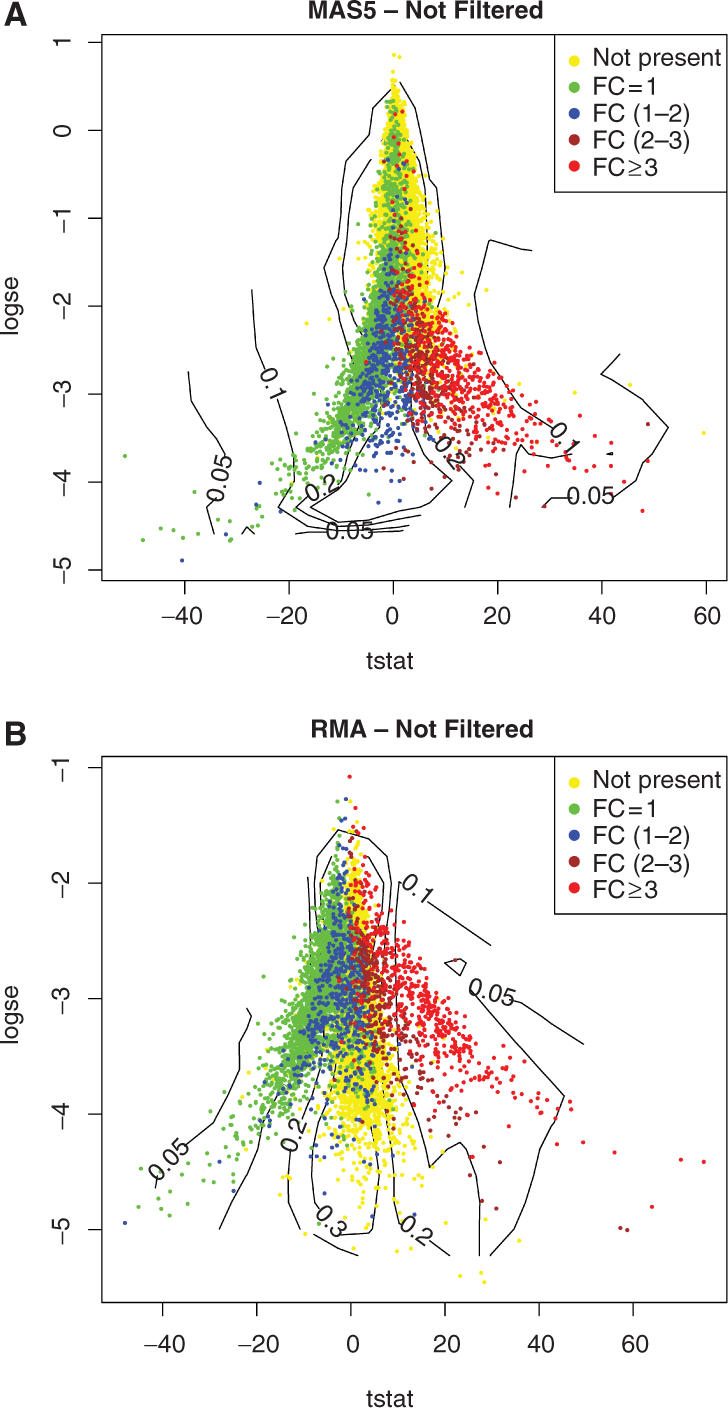
TSE plot for (A) MAS5 and (B) RMA unfiltered values. This plot shows the standard t-statistic on the x-axis and the standard error (in log scale) on the y-axis with additional local fdr isolines (i.e. lines connecting points with the same local fdr value).
Substantial spurious over-expression signal (yellow dots) is evident in both plots, especially in MAS5. This is consistent with previously published analyses that reported a signal content higher than expected (3,20) and might be due to both non-specific binding and normalization bias.
Figure 3 shows the plot of the square-root of the array-effect test statistic as a function of the logarithm of the residual SD—or RA-plot—for the Golden Spike data, showing the array-to-array variability versus residual variance from the probe-level linear model (see ‘Methods’ section). Un-expressed genes showed high residual variance and relatively low array-effects; these correspond to probe sets with inconsistent patterns between replicates. Genes with FC = 1 had low array-effects and relatively low residual variance, but showed some mixing with over-expressed genes. The majority of genes with FC ⩾2 were clearly separated from the cloud of noisy genes.
Figure 3.

RA-plot for Golden Spike data. This plot shows the array-to-array variability versus residual variance from the probe-level linear model. The black line represents the fitted values from a quantile regression with τ = 0.6.
A non-parametric quantile regression smoothing line (see ‘Methods’ section) was fitted using the 60th percentile of array effect as a function of residual SD. As a result of the filtering procedure, a total of 8 400 out of 14 010 features with array effects below the estimated quantile regression line were excluded from further analysis. Given the small sample size, the local fdr estimation through permutation (18) is not completely trustworthy, but the estimated local fdr can still be used to rank genes.
To assess the merits of filtering and to compare the different procedures, we plot in Figure 4 the cumulative number of genes declared DE at increasing values of estimated local fdr, versus the corresponding number of truly DE genes. For the presence-call, intensity and variance filters, we tried to keep almost the same number of genes as for FLUSH. Analyses of unfiltered data suffers from bias as well as large variability due to nonDE genes, resulting in a high number of false discoveries. Presence-call filtering was not able to overcome the biased normalization of non-DE genes, so in this case it performed no better than the unfiltered analysis. The worst performance was demonstrated by the average-intensity and variance filtering, which clearly removed too many truly DE genes. A more restrictive filtering on presence-call was also adopted, selecting features declared present in at least 50% of the samples (13). This produced similar results (see Figure 1S in the Supplementary Report).
Figure 4.

Cumulative distribution of true DE genes versus number of genes declared DE for the various filtering procedures. Criteria for the presence call, average intensity and variance filtering were chosen in order to retain a number of features comparable to the FLUSH method (5 610 genes). Presence-call filtering retained features with at least one presence or marginal call among the six samples (Abs < 100%, 4 899 genes). Both average intensity and variance methods filtered out 60% of genes (5 604 genes kept). The straight line labeled as ‘Random’ represents the expected number of DE identified through a random selection of genes. R is defined as the number of genes declared significant, the number of TDE may be computed as (1−π0)*R, where π0 represents the proportion of non-DE genes. In the Golden Spike data π0 = 90.5%.
In contrast, FLUSH filtering reduced bias, by excluding non-DE genes that were falsely declared DE due to imperfect normalization, and clearly increased the sensitivity of the procedure based on both RMA and MAS5 expression values. For RMA analysis with unfiltered genes, the sensitivity was below 60% regardless of the number of genes declared DE; FLUSH procedure increased the sensitivity to over 80% when considering the top ranked 550 genes declared DE and to 90% for up to 465 genes. For MAS5 analysis with unfiltered genes, the sensitivity was mostly below 60%, while after filtering using FLUSH the sensitivity increased to around 80% for the 450 genes declared DE. Interestingly, unfiltered RMA outperforms unfiltered MAS5, which contrasts with Choe et al. (14). This might be explained by the different normalization approach, i.e. based on the whole set of genes rather than just the non-DE ones.
Mouse-retina degeneration model
We used wild-type C3H mice and inbred C3H rd1/rd1 mutant mice (15) to serve as an animal model for retinal degenerative diseases. Retina was hybridized to Affymetrix GeneChip Mouse Genome 430 2.0 arrays, which contain 45 101 probe sets for over 39 000 well-characterized genes. As for the Golden Spike experiment, the data were processed using both the MAS5 and RMA algorithms, and genes were filtered using FLUSH.
Figure 5 shows the RA-plots of the data. Points were colored according to the quantiles of genes' average expression (on log scale), computed either with the MAS5 or RMA algorithms. Smooth lines (Figure 5C and D) mark the filtering threshold derived from a quantile regression smoothing using τ = 0.4 and λ = δ = 0.45 [see Equation (3)]. As we expected to have relatively few differentially expressed genes in this experiment, we tried to filter most un-informative probe sets. Features lying below the fitted quantile line were filtered out, so that out of 45 101 probe sets, 2 950 were kept. Genes with local fdr (18) lower than 15% for unfiltered features and 5% for filtered ones were printed with variable point size, depending on local fdr values, with larger points having smaller local fdr.
Figure 5.

Filtering of probe sets from a mouse model of retinal degeneration. (A) and (B) show RA-plots for both MAS5 and RMA unfiltered probe sets. Features with fdr < 0.15 have point size related to fdr values with larger dots having smaller fdr. (C) and (D) show the corresponding plots for filtered probe sets. Quantile-regression smoothing was fitted with τ = 0.4 and λ = 0.45. Features with fdr < 0.05 have point size related to fdr values with larger dots having smaller fdr. In all plots, points are colored according to the average intensity computed either on MAS5 or RMA expression values (on logarithmic scale).
For a sensitivity analysis of the choice of filtering parameters, Figure 2S in the Supplementary Report shows the RA-plot of the mouse retina data with four different quantile regression lines, derived from different choices of the tuning parameters. For this range of filtering, the results are not sensitive to the choice of filtering parameters.
Many more genes were assigned a low local fdr value (⩽0.15) by the local fdr procedure (18) applied to RMA values compared to MAS5: 73 probe sets showed a local fdr lower or equal to 0.15 for MAS5 expression values, and 1283 for RMA values (Figure 5A and B). The local fdr estimates for the RMA values are likely biased, as we do not expect to see so many DE genes. It can be seen that many features identified as DE lie in the cloud of probe sets with low array-to-array variability or high residual-variation, and therefore are likely false discoveries. In Figure 5A and B individual spots are color-coded according to probe set signal intensity; it is worth noting that lower intensity features tend to show lower array effects and higher residual variances compared to the high-intensity features.
Figure 5C and D show the same plots of array effect and log residual of SD after filtering using FLUSH. The FLUSH algorithm enhanced the local fdr estimation both for MAS5 and RMA values by putting more emphasis on genes with higher inter-array variability.
Among the FLUSH-filtered DE features we recognized 39 probe sets corresponding to 27 genes known to be regulated during retinal degeneration (21–26). A large majority of these genes are down-regulated, which agrees with the general model of retinal-dysfunction leading to degradation of the photoreceptor layer which can be observed in histological studies in rd1 mice (25). This set of DE genes contains hallmark genes such as RHO (rhodopsin) or PDE6B (phosphodiesterase 6B). PDE6B was previously found to be mutated in rd1 mice (27), and thus gives a non-functional gene-product thought responsible for the onset of retinal degeneration. RHO is the main protein involved in detecting light and is highly abundant in photoreceptor cells. Its abundance decreases towards zero during the process of retinal degeneration (25). Another key enzyme in the regeneration of visual pigments, RDH12 (retinol dehydrogenase 12), was found significantly down-regulated by both probe sets for this gene. This gene codes for the main enzyme involved in converting 11-cis-retinal to 11-cis-retinol in photoreceptor cells.
Also as expected, numerous genes involved in signal transduction and transcriptional regulation were found DE. Among these, CRX (cone-rod homeobox) is known to have a prominent role as photoreceptor-specific transcription factor. In agreement with our model, CRX was down-regulated (28,29).
Several other genes known to play key roles in retinal function and known to be mainly expressed in retina were identified among a stringent selection of 109 probe sets (RMA array-effect χ2 > 292 with local fdr < 0.027): RSG9 (regulator of G-protein signalling 9) and RPGRIP1 (retinitis pigmentosa GTPase regulator interacting protein 1) both play an important role in regulation of G-proteins and maintaining of their proper function. Also the brain and retina-specific G-protein GNGT1 (guanine nucleotide-binding protein, gamma transducing activity polypeptide 1) was found down-regulated together with MAK (male-germ cell-associated kinase) and CDR2 (cerebellar degeneration-related protein 2). Prdx6 (peroxiredoxin 6), whose gene product is involved in immune-response, was found to be up-regulated, in accordance with the stimulation of stress–response and tissue repair mechanisms due to retinal degeneration.
As shown in Figure 6, all 39 known probe sets are located away from the cloud of noisy genes. Some genes known in the context of retinal degeneration had a very low local fdr, but were located closer to the main bulk of points. One example is Gfap (glial fibrillary acidic protein), a well-characterized marker that is almost exclusively expressed in astrocytes and used to follow the progress of retinal degeneration. Overall, FLUSH outperforms the standard FDR method without any filtering. For the RMA expression data, without any filtering, the median ranking of the standard FDR statistic of the 39 previously mentioned probe sets was 902, i.e. the list of 902 top-ranking genes contained only 19 of the 39 probe sets. Since we did not expect so many DE genes, it was clear that these known probe sets were buried among many non-DE genes. After filtering with FLUSH the median ranking was 281 (data not shown), while using the variance filter, the median ranking was 652; this means that variance filter is worse than FLUSH.
Figure 6.

RA-plots of the retina degradation data, where we highlight the probe sets known or suggested to be differentially regulated in rd1 mouse retina at post-natal day 15. Such probe sets are plotted as solid black points and marked with their respective gene symbol.
Variance filtering applied to MAS5 expression values retained only 12 of the 39 probe sets, which means we are likely to lose a lot of DE genes, so we should not use this filter. To understand what happens, Figure 7 shows the location of the genes retained by variance filtering in the RA plot. Comparison with Figure 3 suggests strongly that a large proportion of these genes are likely unexpressed, and inclusion of such genes leads to loss of sensitivity.
Figure 7.

RA-plot of the retina degradation data, where we highlight the probe sets (red points) retained by the variance filtering. In view of Figure 3, these probe sets are likely to correspond to unexpressed genes.
Additionally, we compared our results with an alternative filtering based on the GC-RMA algorithm (30). Using this approach we typically observe a bimodal histogram of intensity values. Since the first of these peaks is (i) very sharp and (ii) part of the lowest signal intensity, it is tempting to associate this peak with non-expressed genes (data not shown). Removing all probe sets with average signal intensity in the first peak (fixed threshold of 4.8) gave 21 231 probe sets. [These correspond to 11 803 different genes, a slightly larger number than the estimate of 9 100-9 200 genes expressed in the retina (31).]
With this filter, the median ranking of standard FDR for the 39 probe sets mentioned above was 998. So, although the histogram-based procedure for GC-RMA removes a large proportion of non-DE probe sets, many unlikely DE probe sets still remain, and thus yield a very high median ranking for the 39 validated probe sets.
DISCUSSION
This article shows a novel data analytic procedure, called FLUSH, for filtering out potentially uninformative genes in Affymetrix microarrays and selecting features with potentially higher information content. FLUSH is meant as a filtering procedure performed in conjunction with any pre-processing step such as normalization and prior to any statistical or DE analysis. The main motivation is that a large proportion of genes on a microarray are un-expressed or non-DE, and these genes make it harder to detect DE genes, so they should be excluded prior to DE analysis. We have shown that FLUSH performs better than other more ad hoc filtering methods based on presence-call or signal intensity. To highlight the novel contributions of FLUSH:
FLUSH operates on raw un-normalized probe-level data, so it is not affected by the biases due to the imperfect normalization step. In fact, the analysis of the spike-in data shows that FLUSH can reduce the effect of biased normalization.
FLUSH is based on the same robust statistical model that provides the RMA expression values, so FLUSH will have the same broad utility as the RMA methodology.
FLUSH produces an informative residual-array (RA) plot that captures the probe-pattern consistency and array-to-array variation. Experience with spike-in and real data suggests that true discoveries are to be found among the extreme points in this plot, so scrutiny of this plot should be part of routine data analysis.
Conceptually, the filtering method we used here can be adapted to other types of microarray data, such cDNA or bead arrays, as long as there are replications for each gene to allow separation of within- and between-array variance. (The within-array variance is the residual variance.) However, because of the assumed data structure, the specific implementation of the method and the R package reported in this article can be applied only to Affymetrix data.
A recent theoretical computation (32) showed that there is an optimal number of hypotheses to be tested that is limited by the number of samples in the experiment. As seen clearly with the data examples, when the proportion of DE genes is small, they tend to get buried among the non-DE genes, thus increasing the FDR. Filtering out likely non-DE genes is a practical solution to this problem.
Our analysis is based on a robust linear model, so it is not affected by outliers generated by some bad samples. Note that the analysis is performed gene by gene, so at any one analysis we expect only a few outliers. Nevertheless, we would recommend that the standard quality control checks for the arrays are followed.
We emphasize that our purpose is not to show whether MAS5 or RMA work for Choe's; data, but whether we gain anything by using FLUSH. In principle, FLUSH can be used with any normalization method. With spike-in data such as Choe's;, it is possible to normalize using the ideal FC1-genes, but this is not feasible in real experiments, where finding FC1 genes requires pre-processed data including the normalization step, so there is a vicious cycle between normalization and finding FC1 genes. Normalization with MAS5 or RMA is usually applied to the full set of genes. The so-called ‘housekeeping-gene normalization’ for MAS5, using the a priori set of FC1 genes, was shown to be biased in Ploner et al. (33). When the FC1-gene normalization was used for RMA as in Choe's; et al. (14), filtering using FLUSH still improves the performance of DE analysis.
In most clinical data, the pattern of over/under-expressed genes tends to be balanced. But in lab experiments, e.g. with knock-out mice, an unbalanced proportion of over/under-expressed genes may reasonably happen. Haslett et al. (34), for example, reported a relevant bias towards over-expression in muscle-related genes (135 of the 185 declared DE). A similar unbalanced pattern was reported in other works (35–38). Such unbalanced over- and under-expression violates the key assumption of balanced expression for the normalization step in data pre-processing. In this situation, both RMA and MAS5 expression measures will be biased due to imperfect normalization. FDR estimation and the sensitivity of the test will be affected by the bias in the pre-processing procedures. The problem is that, with real data sets, it is not obvious whether all the genes have been properly normalized. Even in clinical data with balanced expression levels, Ploner et al.(33) showed that the commonly used quantile normalization is biased for low-intensity genes.
Existing filtering methods based on Affymetrix presence-calls may be useful for removing noisy signal both for MAS5 and RMA values, but as shown in the Golden Spike data analysis, it cannot overcome all possible biases. The proposed FLUSH algorithm flexibly discards likely uninteresting features in terms of low information content (between-array variability), and lack of consistency among probe-pairs within probe sets (residual variance). Unlike variance filtering, FLUSH operates at the raw un-normalized probe-level data, thus it is not affected by the possible bias due to imperfect normalization. From our experience, low intensity genes tend to have higher residual variability, i.e. more inconsistent hybridization patterns across the experimental replicates. FLUSH can account for intensity, since we can use a flexible weight to penalize high residual variance, which is associated with low intensity features.
Filtering genes prior to DE analysis might be viewed with some suspicion, as important differentially regulated features might be lost. There is obviously a sensitivity-specificity trade-off, since without filtering the great amount of spurious signals present in microarray data will make it hard to detect the real information.
Software
All of the statistical analyses was performed using R (39) and Bioconductor (40). The package affyPLM (19) was used for probe-level robust linear model fitting. A freely-available R package called FLUSH implements the procedures and graphical displays described in the paper. The package is available at the authors' website http://www.meb.ki.se/∼yudpaw.
SUPPLEMENTARY DATA
Supplementary Data are available at NAR Online.
ACKNOWLEDGEMENTS
This project is partially supported by a grant from the Swedish Cancer Society. The authors wish to acknowledge the help of Ravi Kiran Reddy Kalathur and critical discussions with Olivier Poch. W.R., J.S. and T.L. were supported by INSERM, CNRS, ULP de Strasbourg and the European Retinal Research Training Network (RetNet) MRTN-CT-20032-504003. Funding to pay the Open Access publication charges for this article was provided by the Swedish Cancer Society and the European Retinal Research Training Network ‘RETNET’ (MRTN-CT-2003-504003).
Conflict of interest statement. None declared.
REFERENCES
- 1.Su AI, Cooke MP, Ching KA, Hakak Y, Walker JR, Wiltshire T, Orth AP, Vega RG, Sapinoso LM, et al. Large-scale analysis of the human and mouse transcriptomes. PNAS. 2002;99:4465–4470. doi: 10.1073/pnas.012025199. [DOI] [PMC free article] [PubMed] [Google Scholar]
- 2.Jongeneel CV, Iseli C, Stevenson BJ, Riggins GJ, Lal A, Mackay A, Harris RA, O'H;are MJ, Neville AM, et al. Comprehensive sampling of gene expression in human cell lines with massively parallel signature sequencing. PNAS. 2003;100:4702–4705. doi: 10.1073/pnas.0831040100. [DOI] [PMC free article] [PubMed] [Google Scholar]
- 3.Dabney A, Storey J. A reanalysis of a published affymetrix genechip control dataset. Gen. Biol. 2006;7:401. doi: 10.1186/gb-2006-7-3-401. [DOI] [PMC free article] [PubMed] [Google Scholar]
- 4.Modlich O, Prisack H-B, Munnes M, Audretsch W, Bojar H. Immediate gene expression changes after the first course of neoadjuvant chemotherapy in patients with primary breast cancer disease. Clin. Cancer Res. 2004;10:6418–6431. doi: 10.1158/1078-0432.CCR-04-1031. [DOI] [PubMed] [Google Scholar]
- 5.Welsh JB, Zarrinkar PP, Sapinoso LM, Kern SG, Behling CA, Monk BJ, Lockhart DJ, Burger RA, Hampton GM. Analysis of gene expression profiles in normal and neoplastic ovarian tissue samples identifies candidate molecular markers of epithelial ovarian cancer. PNAS. 2001;98:1176–1181. doi: 10.1073/pnas.98.3.1176. [DOI] [PMC free article] [PubMed] [Google Scholar]
- 6.Lancaster JM, Dressman HK, Whitaker RS, Havrilesky L, Gray J, Marks JR, Nevins JR, Berchuck A. Gene expression patterns that characterize advanced stage serous ovarian cancers. J. Soc. Gynecol. Investig. 2004;11:51–59. doi: 10.1016/j.jsgi.2003.07.004. [DOI] [PubMed] [Google Scholar]
- 7.Raffelsberger W, Dembele D, Neubauer M, Gottardis M, Gronemeyer H. Quality indicators increase the reliability of microarray data. Genomics. 2002;80:385–94. doi: 10.1006/geno.2002.6848. [DOI] [PubMed] [Google Scholar]
- 8.Bignotti E, Tassi RA, Calza S, Ravaggi A, Romani C, Rossi E, Falchetti M, Odicino FE, Pecorelli S, et al. Differential gene expression profiles between tumor biopsies and short-term primary cultures of ovarian serous carcinomas: identification of novel molecular biomarkers for early diagnosis and therapy. Gynecol. Oncol. 2006;103:405–416. doi: 10.1016/j.ygyno.2006.03.056. [DOI] [PubMed] [Google Scholar]
- 9.Aston C, Jiang L, Sokolov BP. Transcriptional profiling reveals evidence for signaling and oligodendroglial abnormalities in the temporal cortex from patients with major depressive disorder. Mol. Psychiatry. 2005;10:309–312. doi: 10.1038/sj.mp.4001565. [DOI] [PubMed] [Google Scholar]
- 10.Pawitan Y, Bjohle J, Amler L, Borg A-L, Egyhazi S, Hall P, Han X, Holmberg L, Huang F, et al. Gene expression profiling spares early breast cancer patients from adjuvant therapy: derived and validated in two population-based cohorts. Breast Cancer Res. 2005;7:R953–R964. doi: 10.1186/bcr1325. [DOI] [PMC free article] [PubMed] [Google Scholar]
- 11.2002. Affymetrix Statistical Algorithms Description Document. [Google Scholar]
- 12.Irizarry RA, Bolstad BM, Collin F, Cope LM, Hobbs B, Speed TP. Summaries of Affymetrix GeneChip probe level data. Nucl. Acids Res. 2003;31:e15. doi: 10.1093/nar/gng015. [DOI] [PMC free article] [PubMed] [Google Scholar]
- 13.McClintick J, Edenberg H. Effects of filtering by present call on analysis of microarray experiments. BMC Bioinform. 2006;7:49. doi: 10.1186/1471-2105-7-49. [DOI] [PMC free article] [PubMed] [Google Scholar]
- 14.Choe S, Boutros M, Michelson A, Church G, Halfon M. Preferred analysis methods for affymetrix genechips revealed by a wholly defined control dataset. Gen. Biol. 2005;6:R16. doi: 10.1186/gb-2005-6-2-r16. [DOI] [PMC free article] [PubMed] [Google Scholar]
- 15.Viczian A, Sanyal S, Toffenetti J, Chader G, Farber D. Photoreceptor-specific mrnas in mice carrying different allelic combinations at the rd and rds loci. Exp. Eye Res. 1992;54:853–860. doi: 10.1016/0014-4835(92)90148-l. [DOI] [PubMed] [Google Scholar]
- 16.Sambrook J, Fritsch E, Maniatis T. (1989) Molecular Cloning. A Laboratory Manual, 2nd edn. Cold Spring Harbor Laboratory Press, New York. [Google Scholar]
- 17.Glisin V, Crkvenjakov R, Byus C. Ribonucleic acid isolated by cesium chloride centrifugation. Biochemistry. 1974;13:2633–2637. doi: 10.1021/bi00709a025. [DOI] [PubMed] [Google Scholar]
- 18.Ploner A, Calza S, Gusnanto A, Pawitan Y. Multidimensional local false discovery rate for microarray studies. Bioinformatics. 2006;22:556–565. doi: 10.1093/bioinformatics/btk013. [DOI] [PubMed] [Google Scholar]
- 19.Bolstad B. (2006) affyPLM: Methods for fitting probe-level models R package version 1.8.0. [Google Scholar]
- 20.Irizarry RA, Cope L, Wu Z. 2006 Feature level exploration of the choe et al affymetrix genechip control dataset. Technical Report Working Paper 102 Johns Hopkins University, Department of Biostatistics Working Papers. [Google Scholar]
- 21.Jones S, Jomary C, Grist J, Stewart H, Neal M. Identification by array screening of altered nm23-m2/puf mrna expression in mouse retinal degeneration. Mol. Cell Biol. Res. Commun. 2000;4:20–25. doi: 10.1006/mcbr.2000.0250. [DOI] [PubMed] [Google Scholar]
- 22.Rohrer B, Pinto F, Hulse K, Lohr H, Zhang L, Almeida J. Multidestructive pathways triggered in photoreceptor cell death of the rd mouse as determined through gene expression profiling. J. Biol. Chem. 2004;279:41903–41910. doi: 10.1074/jbc.M405085200. [DOI] [PubMed] [Google Scholar]
- 23.Hackam A, Strom R, Liu D, Qian J, Wang C, Otteson D, Gunatilaka T, Farkas R, Chowers I, et al. Identification of gene expression changes associated with the progression of retinal degeneration in the rd1 mouse. Invest. Ophthalmol. Vis. Sci. 2004;45:2929–2942. doi: 10.1167/iovs.03-1184. [DOI] [PubMed] [Google Scholar]
- 24.Azadi S, Paquet-Durand F, Medstrand P, van Veen T, Ekstrom P. Up-regulation and increased phosphorylation of protein kinase c (pkc) delta, mu and theta in the degenerating rd1 mouse retina. Mol. Cell. Neurosci. 2006;31:759–773. doi: 10.1016/j.mcn.2006.01.001. [DOI] [PubMed] [Google Scholar]
- 25.Chang B, Hawes N, Hurd R, Davisson M, Nusinowit ZS, Heckenlively J. Retinal degeneration mutants in the mouse. Vision Res. 2002;42:517–525. doi: 10.1016/s0042-6989(01)00146-8. [DOI] [PubMed] [Google Scholar]
- 26.Dalke C, Graw J. Mouse mutants as models for congenital retinal disorders. Exp. Eye Res. 2005;81:503–512. doi: 10.1016/j.exer.2005.06.004. [DOI] [PubMed] [Google Scholar]
- 27.Bowes C, Li T, Danciger M, Baxter L, Applebury M, Farber D. Retinal degeneration in the rd mouse is caused by a defect in the beta subunit of rod cgmp-phosphodiesterase. Nature. 1990;347:677–678. doi: 10.1038/347677a0. [DOI] [PubMed] [Google Scholar]
- 28.Chen S, Wang Q, Nie Z, Sun H, Lennon G, Copeland N, Gilbert D, Jenkins N, Zack D. Crx, a novel otx-like paired-homeodomain protein, binds to and transactivates photoreceptor cell-specific genes. Neuron. 1997;19:1017–1030. doi: 10.1016/s0896-6273(00)80394-3. [DOI] [PubMed] [Google Scholar]
- 29.Furukawa T, Morrow E, Cepko C. Crx, a novel otx-like homeobox gene, shows photoreceptor-specific expression and regulates photoreceptor differentiation. Cell. 1997;91:531–541. doi: 10.1016/s0092-8674(00)80439-0. [DOI] [PubMed] [Google Scholar]
- 30.with contributions from. Wu J, MacDonald J, Jeff Gentry RI. gcrma: Background Adjustment Using Sequence Information (2006) R package version 2.6.0. 2006 [Google Scholar]
- 31.Blackshaw S, Harpavat S, Trimarchi J, Cai L, Huang H, Kuo WP, Weber G, Lee K, Fraioli RE, et al. Genomic analysis of mouse retinal development. PLoS Biol. 2004;2:E247. doi: 10.1371/journal.pbio.0020247. [DOI] [PMC free article] [PubMed] [Google Scholar]
- 32.Futschik A, Posch M. On the optimum number of hypotheses when the number of observations is limited. Stat Sinica. 2005;15:841–855. [Google Scholar]
- 33.Ploner A, Miller LD, Hall P, Bergh J, Pawitan Y. Correlation test to assess low-level processing of high-density oligonucleotide microarray data. BMC Bioinform. 2005;6:80. doi: 10.1186/1471-2105-6-80. [DOI] [PMC free article] [PubMed] [Google Scholar]
- 34.Haslett JN, Sanoudou D, Kho AT, Han M, Bennett RR, Kohane IS, Beggs AH, Kunkel LM. Gene expression profiling of Duchenne muscular dystrophy skeletal muscle. Neurogenetics. 2003;4:163–171. doi: 10.1007/s10048-003-0148-x. [DOI] [PubMed] [Google Scholar]
- 35.Porter JD, Khanna S, Kaminski HJ, Rao JS, Merriam AP, Richmonds CR, Leahy P, Li J, Guo W, et al. A chronic inflammatory response dominates the skeletal muscle molecular signature in dystrophin-deficient mdx mice. Hum. Mol. Genet. 2002;11:263–272. doi: 10.1093/hmg/11.3.263. [DOI] [PubMed] [Google Scholar]
- 36.Timmons JA, Jansson E, Fischer H, Gustafsson T, Greenhaff PL, Ridden J, Rachman J, Sundberg CJ. Modulation of extracellular matrix genes reflects the magnitude of physiological adaptation to aerobic exercise training in humans. BMC Biol. 2005;3:19. doi: 10.1186/1741-7007-3-19. [DOI] [PMC free article] [PubMed] [Google Scholar]
- 37.Zhou J, Rappaport EF, Tobias JW, Young TL. Differential gene expression in mouse sclera during ocular development. Invest. Ophthalmol. Vis. Sci. 2006;47:1794–1802. doi: 10.1167/iovs.05-0759. [DOI] [PubMed] [Google Scholar]
- 38.Trivedi NR, Gilliland KL, Zhao W, Liu W, Thiboutot DM. Gene array expression profiling in acne lesions reveals marked upregulation of genes involved in inflammation and matrix remodeling. J. Invest. Dermatol. 2006;126:1071–1079. doi: 10.1038/sj.jid.5700213. [DOI] [PubMed] [Google Scholar]
- 39.R Development Core Team. 2006. R: A Language and Environment for Statistical Computing R Foundation for Statistical Computing Vienna. Austria (2006) {ISBN} 3-900051-07-0. [Google Scholar]
- 40.Gentleman RC, Carey VJ, Bates DM, Bolstad B, Dettling M, Dudoit S, Ellis B, Gautier L, Ge Y, et al. Bioconductor: open software development for computational biology and bioinformatics. Gen. Biol. 2004;5:R80. doi: 10.1186/gb-2004-5-10-r80. [DOI] [PMC free article] [PubMed] [Google Scholar]
Associated Data
This section collects any data citations, data availability statements, or supplementary materials included in this article.