Are protein folds atypical?

Abstract

Protein structures are a very special class among all possible structures. It has been suggested that a “designability principle” plays a crucial role in nature’s selection of protein sequences and structures. Here, we provide a theoretical base for such a selection principle, using a simple model of protein folding based on hydrophobic interactions. A structure is reduced to a string of 0s and 1s, which represent the surface and core sites, respectively, as the backbone is traced. Each structure is therefore associated with one point in a high dimensional space. Sequences are represented by strings of their hydrophobicities and thus can be mapped into the same space. A sequence that lies closer to a particular structure in this space than to any other structures will have that structure as its ground state. Atypical structures, namely those far away from other structures in the high dimensional space, have more sequences that fold into them and are thermodynamically more stable. We argue that the most common folds of proteins are the most atypical in the space of possible structures.

Protein structures seem to be a very special class among all possible folded configurations of a polypeptide chain. There are preferred secondary structures and motifs (1) as well as striking regularities in the geometries of protein structures (2, 3). Two proteins are said to have a common fold if they have the same major secondary structures in the same arrangement with the same topological connections (4). Common folds occur even for proteins with different biological functions. Indeed there are “superfolds” (5) and “fold space attractors” (6) that account for the structures of many proteins. It has been estimated that the total number of natural protein folds is only ≈1,000 (7), an extremely small number compared with both the number of proteins and the number of all possible structures. One may ask: Is there anything special about natural protein structures—are they merely an arbitrary outcome of evolution or is there some fundamental reason behind their selection?

Many features of folded proteins can be understood from an energetic point of view (8). Close packing of secondary structures favors some geometrical patterns (9). It has been argued that certain empirical rules for connections between secondary structures can be explained by lower bending energies for the connecting loops (10). It has been conjectured further that a structure with lower energy would stabilize more sequences and would be more likely a protein fold (11). However, the number of low energy structures is huge, and overall low energy does not necessarily imply thermodynamic stability because other low energy structures still compete with the ground state. Clearly, purely energetic considerations are not the whole story.

A recent study on a simple model of protein folding suggested that a rather different mechanism—the so-called “designability principle”—should play a crucial role in nature’s selection of protein sequences and structures (12). The designability of a structure is defined as the number of sequences that possess the structure as their nondegenerate ground state. It was demonstrated in the model that structures with the same low energy (when averaged over sequences) differ drastically in terms of their designability; highly designable structures emerge with a number of associated sequences much larger than the average. These highly designable structures are relatively stable against mutation and are more thermodynamically stable than other structures. In addition, they possess “protein-like” secondary structures and motifs. A number of questions arise: Among the large number of low energy structures, why are some structures highly designable? Why does designability also guarantee thermodynamic stability? Why do highly designable structures have geometrical regularities? Here, we address these questions by using a formulation of protein folding problem based on hydrophobic interactions.

Among the various forces involved in the folding of a polypeptide chain—van der Waals force, electrostatic force, hydrogen bonding, hydrophobic force—there is strong and increasing evidence that the hydrophobic force is the dominant one in determining the overall folded structure (13, 14). The hydrophobic force originates from the contact of nonpolar groups with water, which disrupts the hydrogen bonding exchange pattern between water molecules. Thus, nonpolar groups in water tend to coalesce to minimize their contact with water. For a nonpolar amino acid, the free energy reduction from the hydrophobic interaction is proportional to the total area of the side chain protected from water (15–18). For an amino acid with a polar side chain, there is a smaller reduction because of the possibility of hydrogen bonding between the polar side chain and water molecules (15). To model the hydrophobic force in protein folding, one can assign parameters h_σ to characterize the hydrophobicities of each of the 20 amino acids (19–22). Each sequence of amino acids then has an associated vector h = (h_σ1,h_σ2,…,h_σi,…,h_σN), where σ_i specifies the amino acid at position i of the sequence. We take the energy of a sequence folded into a particular structure to be the sum of the contributions from each amino acid upon burial away from water:

1

where s_i is a structure-dependent number characterizing the degree of burial of the i-th amino acid in the peptide chain.‡ Eq. 1 is essentially a solvation model at the residue level (18, 24, 25). Here, we ignore all other forces that, undoubtedly, help determine the details of the structure of a protein. The advantage of considering only the hydrophobic force is that it drastically simplifies the analysis and thereby elucidates some essential features of the folding problem.

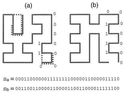
To simplify the application of Eq. 1, let us consider only globular compact structures and let s_i take only two values: 0 and 1, depending on whether the amino acid is on the surface or in the core of the structure, respectively. Therefore, each compact structure can be represented by a string {s_i} of 0s and 1s: s_i = 0 if the i-th amino acid is on the surface and s_i = 1 if it is in the core (see Fig. 1 for an example on a lattice). Assuming every compact structure of a given size has the same numbers of surface and core sites and noting that the term ∑_ih_σ² is a constant for a fixed sequence of amino acids and does not play any role in determining the relative energies of structures folded by the sequence, Eq. 1 is equivalent to:

2

Having rewritten the Hamiltonian 1 in terms of Eq. 2, we now proceed to make a few observations. The problem involves two spaces: the sequence space and the structure space. We represent a sequence by the vector of its hydrophobicities h = (h_σ1,h_σ2,… ,h_σN), and the sequence space {h} consists of 20^N sequences because there can be any of 20 amino acids at each site. A structure also is represented by a vector s = (s₁,s₂,…, s_N), where s_i = 0 or 1, and the structure space {s} consists of all of the structures. Note that only a small subset of the 2^w strings of 0s and 1s represents realizable structures. If two or more structures map into the same string, we say that these structures are degenerate (see Fig. 1a). It is evident that a degenerate structure cannot be the unique ground state for any sequence within this formulation. The fraction of all structures that are nondegenerate depends on the ratio of surface sites to core sites. This fraction approaches zero in the limits of very large and very small surface-to-core ratios. It is worthwhile noting that, for natural proteins, the surface-to-core ratio is of the order one.

Figure 1.

Structures are represented by strings s of 0s and 1s, according to whether a site is on the surface or in the core, respectively. Shown are two examples of compact 6 × 6 lattice structures. (a) A typical structure. Dotted lines indicate local changes that can be performed to transform it to other compact structures. Note that the change at the lower right corner does not change the string pattern, so this structure is a degenerate one. (b) The most designable structure.

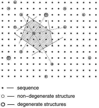
Now imagine embedding both the sequence space {h} and the structure space {s} in an N-dimensional Euclidean space (Fig. 2). This is simplest to picture if one normalizes the h_σ so that 0 ≤ h_σ ≤ 1. Because the energy for a sequence h folded into a structure s is the square of the distance between h and s (Eq. 2), it is evident that h will have s as its unique ground state if and only if h is closer to s than to any other structure. Therefore, the set of all sequences {h(s)} that uniquely design a structure s can be found by the following geometrical construction: Draw bisector planes between s and all of its neighboring structures in the N-dimensional space (see Fig. 2). The volume enclosed by these planes is called the Voronoi polytope around s. {h(s)} then consists of all sequences within the Voronoi polytope. Hence, the designabilities of structures are related directly to the distribution of the structures in the N-dimensional space. A structure closely surrounded by many neighbors will have a small Voronoi polytope and hence a low designability whereas a structure far away from others will have a large Voronoi polytope and hence a high designability. Furthermore, the thermodynamic stability of a folded structure is related directly to the size of its Voronoi polytope. For a sequence h, the energy gap between the ground state and an excited state is the difference of the squared distances between h and the two states (Eq. 2). A larger Voronoi polytope implies, on average, a larger gap because excited states can only lie outside of the Voronoi polytope of the ground state. Thus, this geometrical representation of the problem naturally explains the positive correlation between the thermodynamic stability and the designability, an observation made in ref. 12.

Figure 2.

Schematic plot of the sequence and the structure spaces and the Voronoi construction. The Voronoi polytope is the shaded region.

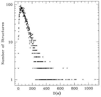
To further illustrate and elaborate on the above ideas, let us proceed with a simple example: a two-dimensional lattice HP model (26). Instead of 20, we use only two amino acids: H (hydrophobic) and P (polar). The vector representing a sequence is now h = (h₁,h₂,… ,h_i,… ,h_N), where h_i = 1 if the i-th amino acid is an H and h_i = 0 if it is a P. The sequence space now consists of all of the possible strings of 0s and 1s of length N. To obtain a set of allowed structure strings, we focus on the compact 6 × 6 two-dimensional lattice structures (Fig. 1), which can be enumerated easily. We divide the 36 sites into 20 surface sites and 16 core sites; the surface-to-core ratio is 1.25. There are 57,337 compact structures not related by symmetries. These structures map into 30,408 distinct strings, among which 18,213 (≈30% of all structures) represent nondegenerate structures. To obtain a histogram of the designability for all structures, we randomly sampled the sequence space. We randomly chose ≈20 million sequences (enough to suppress statistical fluctuations), and for each of these, we calculated its energy on all of the structure strings by using Eq. 1. We found that ≈8.8% of all of the sequences chosen have unique ground states, i.e., they fall inside of the Voronoi polytope of some nondegenerate structure. The designability histogram obtained in the sampling is plotted in Fig. 3. Recall that the designability of a structure D(s) is the number of sequences found to have that structure as their unique ground state. The designabilities obtained from this model are very well correlated with those found in the previous work (12), which were obtained from a different HP model, and with those calculated by using the Miyazawa–Jernigan interaction matrix (23) for all 20 amino acids. The sets of highly designable structures are essentially the same for all three models.

Figure 3.

Histogram of the designability obtained by random sampling by using 19,492,200 sequences.

Certain features of Fig. 3 can be understood from the following simple consideration. If the structure strings were distributed randomly in the N-dimensional space, then one would expect the distribution of the volumes V of the Voronoi polytopes constructed around every structure to be ∝exp(−cV), for cV ≫ 1, where c is proportional to the overall density of structure strings (27). Moreover, the probability of finding very small Voronoi volumes V would also vanish because small Vs require a close clustering of randomly distributed points§. The distribution shown in Fig. 3 indeed has a rising part for small designability D and a decaying part that is roughly exponential. However, one should not conclude from this that the structures are randomly distributed. In fact, the structures are highly correlated and clustered. For example, in Fig. 3, there are structures [with D(s) > 500] that are highly designable and that do not follow the exponential decay.

To more fully understand the designabilities of structures, one has to know the distribution of structures in the N-dimensional space. Each realizable string s represents one (sometimes more than one) globular compact structure; its components s_i are determined by the geometry of the represented structure. One trivial correlation between the realizable strings comes from the constraint that Σ_is_i = n_c, where n_c is the number of core sites and is a constant depending only on N. Therefore, {s} reside in a subspace consisting of those strings whose Hamming distance¶ to the origin equals n_c. Other more subtle correlations are related to the properties of compact self-avoiding walks of length N. To characterize the ensemble properties of {s}, we measure the correlation function c(i,j) = 〈s_is_j〉 − 〈s_i〉〈s_j〉, where the average is taken over all 57,337 compact structures. In Fig. 4, c(i,j) is plotted vs. j−i for three different starting positions: i = 1, i = 9, and i = 18. A common feature of these correlation functions is that s_i has positive correlation with nearby sites and that the correlation turns negative as j−i increases. This feature simply reflects a property of self-avoiding random walks in a confined geometry: If a site is in the core then most likely the next few sites are also in the core, and similarly if a site is on the surface, the next few sites are most likely on the surface. From Fig. 4 we see that the transition between core and surface takes, on average, approximately four to six steps. The residual negative correlation at large distances is a result of the constraint that there is a fixed number of core (and surface) sites.

Figure 4.

Correlation functions for the structures.

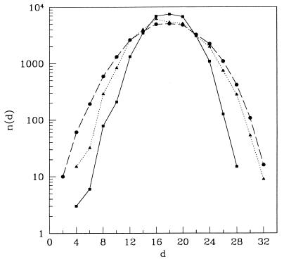
Another way to measure the correlation of the structures is to measure the number of distinct structure strings, n_s(d), at a Hamming distance d from a given string s. In Fig. 5, n_s(d) is plotted for three different structures with low, intermediate, and high designabilities, respectively. A highly designable structure typically has fewer neighbors than a less designable structure, not only at the smallest ds but out to ds of order 10–12. This result indicates that there exists a local “density” around each structure in the N-dimensional space.

Figure 5.

Number of structures vs. the Hamming distance for three structures with: low (circles), intermediate (triangles), and high (squares) designability.

From the above discussion, we see that structure strings are not distributed randomly in the N-dimensional space. Their distribution is highly correlated. There are high density regions as well as regions with very low density. High density regions consist of “typical” structures or typical random walks (see Fig. 1a for an example) whose correlation functions are similar to the correlation function of the ensemble (Fig. 4). These structures usually have small Voronoi polytopes because they are closely surrounded by many neighbors. “Atypical” or “rare” structures reside in regions with very low local density, and their correlation functions are generally very different from Fig. 4. Atypical structures usually have high designabilities because they are relatively far away from other structures or have fewer neighbors. One way for a structure to have an atypical correlation function is to have many surface-to-core transitions along its backbone. This leads to geometrically regular pleated patterns such as the one shown in Fig. 1b, which is in fact the most designable structure. Thus, the emergence of the “protein-like” sub-structures and motifs in the highly designable structures (12) occurs not because they are common but precisely because they are rare. A related property of rare structures, which follows from the large Voronoi polytope, is that it is hard to make any local change to them. For the “typical” structure in Fig. 1a, one can make local changes as indicated by the dotted lines to transform the structure to other compact structures. It is impossible to perform any such local changes for the most designable—and therefore most “atypical”—structure in Fig. 1b.

In conclusion, a simple solvation model leads to a geometrical formulation of the protein folding problem. A very simple and transparent picture emerges from the formulation in which the designability of a structure, i.e., the number of sequences for which the structure is a unique ground state, is directly related to the volume of the Voronoi polytope around the structure. Structures with atypical patterns of surface and core sites have high designability and are generally more stable thermodynamically. These atypical patterns produce geometrically regular structures with “protein-like” motifs. According to this picture, the most common folds in natural proteins are the most atypical in the space of possible structures. Note that highly designable structures do not have lower energies than other structures. It is easy to see from Eq. 1 that the average energy and the energy spectrum (over all the sequences) are the same for all the compact globular structures. Thus, a structure is highly designable in our model, not because it has a lower energy or an unusual energy spectrum as conjectured by Finkelstein and colleagues (11), but because it is far away from neighboring competing structures in the N-dimensional space. In our discussion, we considered only the hydrophobic interaction and compact globular structures. The formulation can be generalized, at least conceptually, without much difficulty to include noncompact structures and main-chain hydrogen bonding, both of which are purely structural properties. The overall picture is unchanged. Our results can be tested on real protein structures. For a globular protein, there is a natural division into core and surface sites and thus a string representation. The strings of natural proteins can be compared with the ensemble of strings of random structures. The knowledge of the distribution of structures in the N-dimensional space can be used to aid protein structure classification, protein design, and structure prediction.

References

- 1.Levitt M, Chothia C. Nature (London) 1976;261:552–558. doi: 10.1038/261552a0. [DOI] [PubMed] [Google Scholar]
- 2.Richardson J S. Proc Natl Acad Sci USA. 1976;73:2619–2623. doi: 10.1073/pnas.73.8.2619. [DOI] [PMC free article] [PubMed] [Google Scholar]
- 3.Richardson J S. Adv Protein Chem. 1981;34:167–339. doi: 10.1016/s0065-3233(08)60520-3. [DOI] [PubMed] [Google Scholar]
- 4.Murzin A G, Brenner S E, Hubbard T, Chothia C. J Mol Biol. 1995;247:536–540. doi: 10.1006/jmbi.1995.0159. [DOI] [PubMed] [Google Scholar]
- 5.Orengo C A, Jones D T, Thornton J M. Nature (London) 1994;372:631–634. doi: 10.1038/372631a0. [DOI] [PubMed] [Google Scholar]
- 6.Holm L, Sander C. Science. 1996;273:595–603. doi: 10.1126/science.273.5275.595. [DOI] [PubMed] [Google Scholar]
- 7.Chothia C. Nature (London) 1992;357:543–544. doi: 10.1038/357543a0. [DOI] [PubMed] [Google Scholar]
- 8.Chothia C, Finkelstein A V. Annu Rev Biochem. 1990;59:1007–1039. doi: 10.1146/annurev.bi.59.070190.005043. [DOI] [PubMed] [Google Scholar]
- 9.Chothia C, Levitt M, Richardson D. Proc Natl Acad Sci USA. 1977;74:4130–4134. doi: 10.1073/pnas.74.10.4130. [DOI] [PMC free article] [PubMed] [Google Scholar]
- 10.Finkelstein A V, Ptitsyn O B. Prog Biophys Mol Biol. 1987;50:171–190. doi: 10.1016/0079-6107(87)90013-7. [DOI] [PubMed] [Google Scholar]
- 11.Finkelstein A V, Gutun A M, Badretdinov A Ya. FEBS Lett. 1993;325:23–28. doi: 10.1016/0014-5793(93)81407-q. [DOI] [PubMed] [Google Scholar]
- 12.Li H, Helling R, Tang C, Wingreen N. Science. 1996;273:666–669. doi: 10.1126/science.273.5275.666. [DOI] [PubMed] [Google Scholar]
- 13.Kauzmann W. Adv Protein Chem. 1959;14:1–63. doi: 10.1016/s0065-3233(08)60608-7. [DOI] [PubMed] [Google Scholar]
- 14.Dill K A. Biochemistry. 1990;29:7133–7155. doi: 10.1021/bi00483a001. [DOI] [PubMed] [Google Scholar]
- 15.Chothia C. Nature (London) 1974;248:338–339. doi: 10.1038/248338a0. [DOI] [PubMed] [Google Scholar]
- 16.Hermann R B. J Phys Chem. 1972;76:2754–2759. [Google Scholar]
- 17.Richards F M. Annu Rev Biophys Bioeng. 1977;6:151–176. doi: 10.1146/annurev.bb.06.060177.001055. [DOI] [PubMed] [Google Scholar]
- 18.Eisenberg D, McLachlan A D. Nature (London) 1986;319:199–203. doi: 10.1038/319199a0. [DOI] [PubMed] [Google Scholar]
- 19.Nozaki Y, Tanford C. J Biol Chem. 1971;246:2211–2217. [PubMed] [Google Scholar]
- 20.Levitt M. J Mol Biol. 1976;104:59–107. doi: 10.1016/0022-2836(76)90004-8. [DOI] [PubMed] [Google Scholar]
- 21.Roseman M A. J Mol Biol. 1988;200:513–522. doi: 10.1016/0022-2836(88)90540-2. [DOI] [PubMed] [Google Scholar]
- 22.Li H, Tang C, Wingreen N S. Phys Rev Lett. 1997;79:765–768. [Google Scholar]
- 23.Miyazawa S, Jernigan R L. J Mol Biol. 1996;256:623–644. doi: 10.1006/jmbi.1996.0114. [DOI] [PubMed] [Google Scholar]
- 24.Kocher J-P A, Rooman M J, Wodak S J. J Mol Biol. 1994;235:1598–1613. doi: 10.1006/jmbi.1994.1109. [DOI] [PubMed] [Google Scholar]
- 25.Park B, Levitt M. J Mol Biol. 1996;258:367–392. doi: 10.1006/jmbi.1996.0256. [DOI] [PubMed] [Google Scholar]
- 26.Lau K F, Dill K A. Macromolecules. 1989;22:3986–3997. [Google Scholar]
- 27.Gilbert E N. Ann Math Stat. 1962;33:958–972. [Google Scholar]
- 28.Hinde A L, Miles R E. J Stat Comput Simul. 1980;10:205–223. [Google Scholar]
- 29.Kumar S, Kurtz S K, Banavar J R, Sharma M G. J Stat Phys. 1992;67:523–551. [Google Scholar]