

Abstract
Electron paramagnetic resonance imaging (EPRI) provides direct detection and mapping of free radicals. The continuous wave (CW) EPRI technique, in particular, has been widely used in a variety of applications in the fields of biology and medicine due to its high sensitivity and applicability to a wide range of free radicals and paramagnetic species. However, the technique requires long image acquisition periods, and this limits its use for many in vivo applications where relatively rapid changes occur in the magnitude and distribution of spins. Therefore, there has been a great need to develop fast EPRI techniques. We report the development of a fast 3D CW EPRI technique using spiral magnetic field gradient. By spiraling the magnetic field gradient and stepping the main magnetic field, this approach acquires a 3D image in one sweep of the main magnetic field, enabling significant reduction of the imaging time. A direct one-stage 3D image reconstruction algorithm, modified for reconstruction of the EPR images from the projections acquired with the spiral magnetic field gradient, was used. We demonstrated using a home-built L-band EPR system that the spiral magnetic field gradient technique enabled a 4 to 7-fold accelerated acquisition of projections. This technique has great potential for in vivo studies of free radicals and their metabolism.
Keywords: fast 3D EPRI, free radicals, image reconstruction, spiral magnetic field gradient, trityl
INTRODUCTION
Electron paramagnetic resonance imaging (EPRI) provides a direct way to detect and map free radicals in a variety of biomedical applications (1–8) . It can be performed in either pulse mode (time-domain) or continuous wave (CW) mode. The pulse mode, which is similar to magnetic resonance imaging (MRI), allows fast image acquisition and therefore minimizes animal motion artifacts (9). But it requires the use of narrow-line spin probes such as trityl radicals. On the other hand, the CW mode enables the use of a variety of spin probes and still dominates current applications (10). However, due to the nature of field sweep, the imaging time in CW EPRI is relatively long (11). For example, it typically takes several minutes for a conventional EPR imaging system to acquire a 2D image and tens of minutes for a 3D image (12). The long imaging time prevents the use of this technique for many biological applications where the free radicals have a short lifetime or a rapid metabolic clearance (13). Therefore, there has been increasing interest in developing fast EPRI techniques (14–17).
To reduce the long imaging time in CW EPRI, many fast field-scanning techniques have been reported. Demsar et al have demonstrated the use of a fast acquisition in detection of diffusion and distribution of oxygen (14). In 1996, Oikawa et al developed a fast EPRI system based on the fast field-scanning technique (15), which was able to acquire a 3D image in 1.5 min using 81 projections. Another approach to accelerate CW EPRI image acquisition has been to spin the magnetic field gradient. In this technique, the gradients are continuously changed during projection collection while the main magnetic field is stepped. Ohno and Watanabe (16) first reported a fast 2D EPR imaging method using spinning magnetic field gradients and demonstrated the feasibility of imaging two small crystals of lithium phthalocyanine (LiPc) at χ-band. Recently, we have implemented this technique at 300 MHz (17) enabling acquisition of good quality 2D images in a significantly reduced imaging time. In comparison with the fast field scanning technique that requires a specialized field-scanning coil and the related compensation algorithm, the technique of spinning magnetic field gradient has the advantage of a relatively low hardware requirement. In principle, no modifications need to be made to the existing magnet and gradients of a conventional EPRI system. The only requirement is that the gradients have a low inductance and sufficiently rapid response time (17).
In this paper, we report a fast 3D CW EPRI technique using spiral magnetic field gradient. We report both hardware and software approaches to implement the spiral magnetic field gradient technique to achieve fast 3D EPR imaging at L-band. The gradient waveforms and the field control signal were generated using high-performance data acquisition boards. The one-stage 3D image reconstruction algorithm (18, 19) was modified to reconstruct the EPR images directly from the projections acquired using spiral magnetic field gradient. We compared the method to the standard stepped magnetic field gradient approach and showed that marked acceleration of image acquisition can be realized in 3D CW EPRI by the spiral magnetic field gradient technique.
THEORY
3D EPRI Using Stepped Magnetic Field Gradients
A projection in conventional 3D EPRI is defined (18) by the following equation:
| [1] |
where α and θ define the direction of the gradient vector in a polar coordinate system and s is the distance from the coordinate origin to the integral plane on which the resonance occurs. In experiments, a projection is acquired by fixing the gradient vector (fixing α and θ ) and sweeping the main magnetic field. The field sweep moves the integral plane along the gradient vector axis to cover the whole 3D object. To collect all the projections, the gradient is rotated in discrete steps (20) by changing the gradient angles, α and θ .
A direct one-stage image reconstruction algorithm can be used to reconstruct the EPR image (19). First, all the projections are filtered using a 3-point digital filter,
| [2] |
where 0 ≤i ≤I −1, 0 ≤j ≤J −1 and 0 ≤k ≤K −1. I is the number of data points in each projection. J and K are the number of steps of the gradient angles α and θ , respectively. Then, the filtered projections are back-projected to obtain the reconstruction result:
| [3] |
Fast 3D EPR Imaging Using Spiral Magnetic Field Gradient
As noted in the previous section, in conventional 3D EPRI, the projection data p(si, αj, θk), is acquired through 3-layer nested loops with the inner loop for field sweep and the outer two loops for gradient angles α and θ , respectively. This is shown as “χ” marks in Fig. 1 for the gradient distribution in conventional EPRI. The field sweep is repeatedly carried out for each α and θ combination during projection collection. For a given number of projections to acquire, the image acquisition time is determined by the speed of field scanning, assuming reasonable signal-to-noise ratio is achieved. Unfortunately, most magnets used in EPRI have a relatively long response time and are not suitable for fast field sweeping. To avoid this problem, the field sweep loop is placed as the outer loop, as previously reported (16, 17) for 2D fast EPRI. A pseudo projection is then acquired by fixing s (the magnetic field) and continuously changing the gradient angles α and θ (spiraling the magnetic field gradient). In this case, the imaging time is determined by the speed of the spiraling of the gradient vector, which can readily reach to as high as tens of Hertz without special hardware modifications to the existing gradient coils that are operated in non-resonant mode. In principle, the spiraling magnetic field gradient technique has a fundamental advantage over the standard stepped gradient acquisition, in that it enables the acquisition of an unlimited number of projections in one field sweep of the main magnet rather than requiring a field sweep for each projection.
Fig. 1.
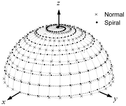
Stepped magnetic field gradients vs. a spiral magnetic field gradient for 3D image acquisition. In the stepped gradients data acquisition, the gradient angles θ and α are changed through a two-layer loop and the projections are acquired at the positions marked by “χ”. In the spiral gradient data acquisition, the gradient vector is spiraling along the dotted line from the bottom to the top of the semi-sphere. The projections are acquired at the positions represented by the solid dots “•” on the semi-sphere.
Gradient Waveform Generation
The magnetic field gradients for 3D spiral EPRI are given by
| [4] |
where G is the gradient strength represented in voltage, Cx , Cy and Cz are gradient strength compensation coefficients (17), f1 is the rotation frequency of the transverse gradient component in the transverse plane (xy-plane), and f2 is the precession frequency of the longitudinal gradient component. f1 and f2 are chosen such that when the longitudinal gradient component precesses from the transverse plane to the longitudinal axis (z-axis), the transverse gradient component will rotate m full cycles in the transverse plane, i.e. f1 =4m · f2 , where m is an integer. The constant 4 is due to the fact that within the same time the longitudinal gradient component precesses only cycle (90°) while the transverse gradient component rotates m full cycles. The gradient vector spiraling on a semi-sphere is shown as the dotted line in Fig. 1 for m =8.
Modified One-stage 3D Image Reconstruction
The EPR signal is digitized and stored as pseudo projections. All the pseudo projections are smoothed, down-sampled and re-ordered to form normal-mode projections (17). The distribution of the re-ordered projections is shown as solid dots “•” in Fig. 1. Since α and θ are simultaneously changed during data collection, the projections acquired with the spiral gradient have different distribution compared to those acquired using stepped magnetic field gradients. As a result, Eq. [3] can not be directly used to reconstruct images from these re-ordered, normal-mode projections. Thus, we modify Eq. [3] as
| [5] |
where W is the weight coefficient, defined as
| [6] |
for image reconstruction.
MATERIALS AND METHODS
The Phantom
We used an ethoxycarbonyl derivative of tetrathiatriarylmethyl radical synthesized as described (21). An aqueous solution of sodium salt of trityl radical (2 mM) was prepared by dissolving it in water and the pH was adjusted to neutral. The peak-to-peak linewidth of the trityl in room air was 19 μT at L-band. A phantom was constructed using 7 syringe tubes (id = 4 mm) after removal of the metal needle. Each tube was filled with 0.2 ml trityl solution. The filling length of the trityl solution was approximately 20 mm. Each tube was separated from the others by about 6.9 mm (center-to-center distance).
The L-Band EPR Imaging System
A home-built L-band EPR imaging system was used. The L-band imaging system is similar to our 300 MHz imaging system (17), except that the microwave bridge and the resonator were specially designed to work at L-band, as described below. A solenoid electromagnet design with field homogeneity of about 3 ppm over a 10 cm DSV (diameter of spherical volume) was used. The magnet was originally designed for use in nuclear magnetic resonance imaging (22). The gradient system used (BFG-U-140-25, Resonance Research Inc., Billerica, MA) offers a gradient linearity better than 1% over an 80 mm DSV. A reflection-type bridge was used in the experiments which consisted of a cavity stabilized transistor oscillator, isolators, 3-port circulator, directional coupler and 60 dB variable attenuator (4). Up to 250 mW microwave power was available from the bridge. A Herotek (Herotek Inc., San Jose, CA) DSL-102p Schottky detector-limiter was used for RF detection. The detector diode signal was connected to a preamplifier, which passed both the 100 kHz field modulation signal to a Bruker ER-023 (Bruker BioSpin, Billerica, MA) lock in amplifier, and the automatic frequency control modulation signal to the AFC system. A Hafler (Rockford Corp., Tempe, AZ) P3000 audio power amplifier received modulation excitation from the ER-023 lock-in amplifier and provided 100 kHz magnetic field modulation. Over 0.2 mT of field modulation was available with the outer modulation coils operating in a non-resonant mode. A 4-gap loop-gap resonator was used in the experiments, which was constructed entirely with plastic. To ensure mechanical stability, the resonator core was constructed from 4 silver electroplated Rexolite prisms arranged around an inner cylinder. This sub assembly was then pressed into another PVC plastic cylinder, which became the outer diameter of the resonator assembly to form a mechanically stable monolithic-like structure. The outer cylinder was painted with a conductive paint to act as an electrical shield. Inner resonator dimensions were 28 mm in diameter and 25 mm in length. The outer diameter was 66 mm. The resonant frequency was about 1.08 GHz and the Q factor was 200 without loading and 180 with loading of the trityl phantom.
Waveform Generation and Synchronization
A personal computer (PC) equipped with one PCI-488 board (Capital Equipment Corporation, MA) and three KPCI-3116 boards (Keithley Instruments, Inc., OH) was used to control the gradients, the field sweep and the EPR signal acquisition. As in our other EPR imaging systems (12, 23), the Bruker signal channel was interfaced with the computer through the PCI-488 GPIB card. The KPCI-3116 boards are high-performance data acquisition boards capable of 16-bit digital-to-analog (D/A) and/or analog-to-digital (A/D) conversion paced by either internal or external clock. They were used to output the field sweep signal and the gradient waveforms. Since each KPCI-3116 board had only two D/A outputs, three boards were used to obtain up to 6 analog outputs. Among these 6 D/A channels, three were used for x, y and z gradient control. We improved the field control by using separate D/A channel for the central field and the field sweep. To maximize the utilization of the dynamic voltage range (±10 V) of the board, the field sweep signal was amplified by a factor of 20 before D/A conversion and later attenuated by the same factor. The attenuated field sweep signal and the central field signal were summed and fed to the magnetic field power supply (see the dashed box at the bottom of Fig. 2). For synchronization purpose, all three KPCI-3116 boards were programmed to work in the external clock mode. The external clock signal was generated through the internal timer 1 and 2 (cascaded) of board 1 (see Fig. 2). In this way, the three KPCI-3116 boards were synchronized. During the experiments, the analog input subsystem (AI) of Board 2 was also activated to digitize the EPR signal coming from the analog output of the Bruker signal channel. The pacing frequency for D/A and A/D conversion was 10 kHz in our experiments.
Fig. 2.
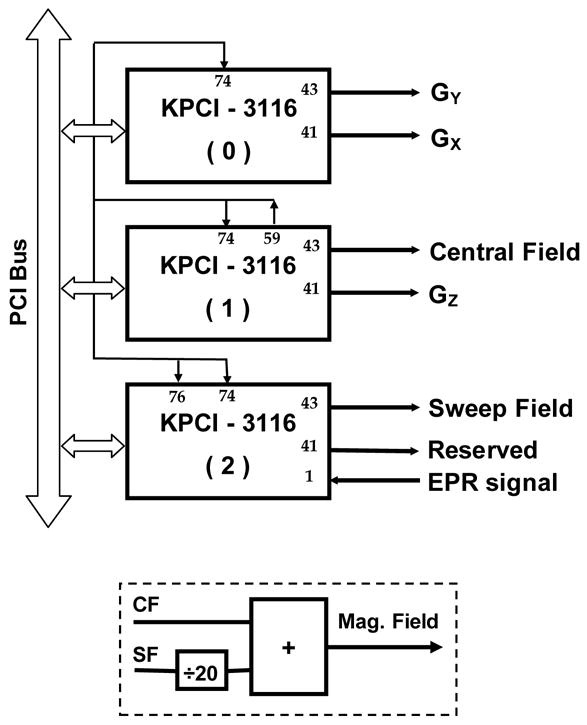
Diagram of magnetic field control and gradient waveform generation using KPCI-3116 boards. All the KPCI-3116 boards are programmed to work in external clock mode. Pin 59 of board 1 outputs a square waveform that is used as an external clock (through pin 74). The field sweep signal is amplified by a factor of 20 before D/A conversion and later attenuated by the same factor using an attenuator. The attenuated field sweep signal and the central field signal are summed and fed to the magnetic field power supply. The analog EPR signal is sampled through the pin 1 of board 2. The pacing frequency for D/A and A/D is 10 kHz.
Before starting the imaging experiments, the field control signal and the magnetic field gradient waveforms were calculated according to the imaging parameters and stored in a chain of buffers that were accessible by the KPCI-3116 boards. Extra waiting periods were inserted in between two successive field steps to avoid discontinuous current change in the gradient coils. Fig. 3 shows the waveforms for gradient and field control. During the experiments, the stored field control signal and the gradient waveforms were output to drive the main magnetic field power amplification and the gradient power amplification, respectively. In the meantime, the EPR signal (analog output from the Bruker signal channel) was sampled at 10 kHz frequency and stored in computer for post-processing.
Fig. 3.
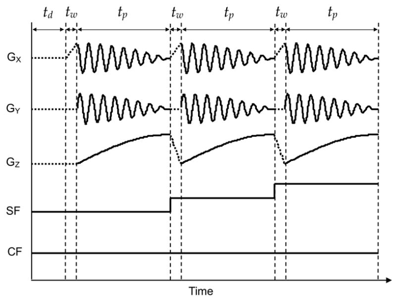
Waveforms for gradients and field control. td, tw and tp represent delay time, waiting time and pseudo projection acquisition time, respectively. The waveforms for field sweep and magnetic field gradient are calculated according to the imaging parameters and stored in buffers that are accessible by the KPCI-3116 boards. Extra waiting periods are inserted in between two successive field steps to avoid abrupt current change in the gradient coils. The stored waveforms are output to drive the main magnetic field power amplification and the gradient power amplification.
Projection Acquisition
We implemented the 3D fast EPR imaging system using spiral magnetic field gradient, and tested it on our home-built L-band CW EPRI system. We carried out both regular and fast EPR imaging experiments on a phantom for validation and comparison. In the regular imaging experiments using stepped gradients, the main magnetic field was swept continuously and a fixed length of 1024 points was acquired for each projection. The total image acquisition time was determined by the product of the scan time with the number of projections. However, with the existing solenoidal magnet and the current-regulated magnetic field control technique, the shortest scan time that could be used was 2.6 s. This limitation was primarily due to the time constant of the magnet and the EPR signals were distorted with scan times less than 2.6 s. In the fast imaging experiments, the imaging time was controlled by the number of steps of field sweep and the spiral frequency, but not by the number of projections as in the stepped gradient acquisitions. In both regular and fast imaging experiments, the scan width = 1.6 mT and FOV = 40x40x40 mm3, resulting in a gradient strength of 40 mT/m. The modulation frequency was 100 kHz and the modulation amplitude was 20 μT. The time constant was 5 ms for the regular data acquisition and 0.64 ms for the spiral data acquisition in the experiments. The incident microwave power was 40 mW and no saturation was observed on the phantom. The peak-peak signal-to-noise ratio (SNR) of the observed zero-gradient spectrum was > 1,000 for a 2.6 s acquisition. The image resolution was approximately 0.9 mm (24) and could be enhanced by a factor of 2–3 after deconvolution (25).
Data Post-processing and Image Reconstruction
The home-built software “EPR2000” was used to control the data acquisition, postprocessing and image reconstruction. This Windows program was developed using Microsoft Visual C++ plus Matlab C++ libraries. The data points corresponding to the delay time, td , at the beginning of data acquisition and the waiting cycle, tw , in between two successive field steps were removed. The data points corresponding to the time tp were extracted to obtain the pseudo projections. The length of each pseudo projection, i.e. the sampling frequency (10 kHz) divided by 4 times the precessional frequency f2 , determined the number of the normal-mode projections after data re-ordering. To reduce the time for data post-processing and image reconstruction, each pseudo projection was down-sampled. The down-sampling rate was chosen such that J ≈4 · K holds true, which was desired for 360°–90° acquisition. Finally, a total of J ·K normal-mode projections, each with I data points, were obtained, as illustrated by the solid dots “•” in Fig. 1. Each projection was further filtered using a 3rd order Savitzky-Golay filter before image reconstruction. As in conventional EPR imaging experiments, a zero-gradient projection was also acquired. The automatic deconvolution algorithm (26) was used to deconvolve all the projections. The modified one-stage image reconstruction, discussed in the THEORY section, was used to reconstruct the EPR images.
RESULTS
The regular images acquired using stepped gradients are shown in Fig. 4A-D. The projection number for Fig. 4A-D was 144, 256, 400 and 576, respectively. Each projection was acquired with 2.6 s scan time plus 0.1 s delay between scans. Therefore, the total imaging time was 392, 696, 1088 and 1567 s, respectively. Fig. 4A’-D’ show the imaging results of the same phantom using the comparable spiral magnetic field gradient technique. The number of steps of field sweep was 128 and the spiral frequency pair f1 (f2) were 24.39 (0.554), 24.10 (0.287), 12.05 (0.143) and 12.27 (0.075) Hz, respectively. The down-sampling rate was 10, 5, 10 and 5, respectively. The imaging time was 58, 111, 223 and 428 s, respectively, within which 451, 1743, 1743 and 6683 projections were acquired. From Fig. 4, it can be seen that with this trityl phantom, at least 1088 s (400 projections) were needed to achieve reasonably good image using the stepped gradients data acquisition. This minimum time, however, could be reduced to 223 s, even 111 s, by using the spiral gradient data acquisition. To quantitatively compare the image quality, the signal-to-noise ratio (SNR) for each 3D image was calculated. The SNR was defined as the mean of the signal (>10% of the maximum signal intensity) divided by the standard deviation of the noise (<10% of the maximum signal intensity but greater than 0). Table 1 summarizes the results of image analysis. The SNR and imaging time of the images are also plotted in Fig. 5A and B, respectively. From Figs. 4 and 5, it can be seen that, in the regular imaging experiments, the image quality was poor when only 144 projections were used (Fig. 4A, 392 s, SNR = 7.7). Increasing the projection number to 256 increased the SNR from 7.7 to 10.9 (Fig. 4B, 696 s). However, 400 projections (Fig. 4C, 1088 s) were needed in actual imaging applications to achieve desirable image quality. The longest imaging time produced the highest SNR and the best image quality (Fig. 4D, 576 projections and 1567 s, SNR = 29.3). However, this may not be feasible in some applications due to the fast metabolic clearance of the free radicals and/or the instability of the imaging system. Compared with the stepped gradients imaging technique, the spiral EPRI technique was able to greatly reduce the image acquisition time. For example, within 58 s, a reasonable 3D EPR image (Fig. 4A’, SNR = 16.5) was obtained, whose SNR was twice that of the image acquired in 392 s using stepped gradients (Fig. 4A, SNR = 7.7). From a practical application point of view, 223 s may be needed (Fig. 4C’, SNR = 26.4) to obtain good image quality using spiral gradient under the conditions used in the measurements. The 223-second spiral image was better than the 1088-second regular image and there was no detectable difference between the 1567-second regular image and the 428-second spiral image though the former has a slightly higher SNR. Thus, we demonstrated that for a relatively strong sample, a 4–7 fold acceleration of image data collection was achieved in 3D fast EPRI experiments.
Fig. 4.
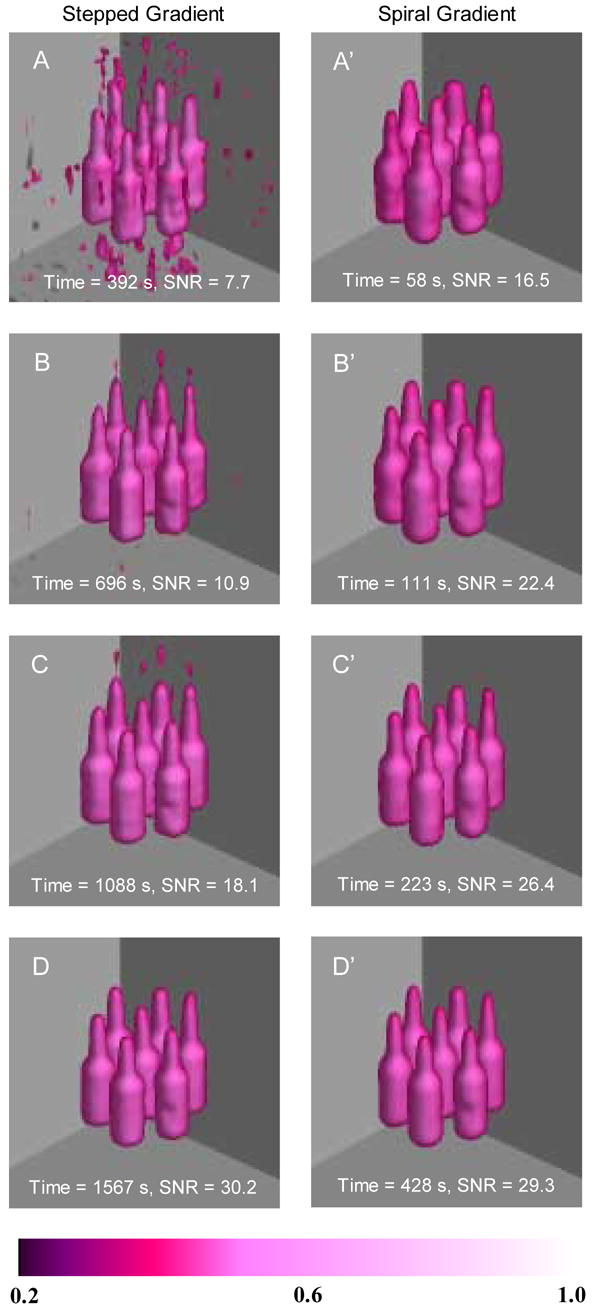
Imaging results of phantom. A phantom consisting of 7 syringe tubes (id = 4 mm) each filled with 0.2 ml of 2 mM trityl solution was used. Images A-D are regular images acquired with stepped magnetic field gradients. The imaging parameters were: scan width = 1.6 mT, FOV = 40x40x40 mm3, gradient strength = 40 mT/m, modulation frequency = 100 kHz, modulation amplitude = 20 μT, incident microwave power = 40 mW, scan time = 2.6 s and time constant = 5 ms. The number of projections were 144, 256, 400 and 576, corresponding to imaging time 392, 696, 1088 and 1567 s, respectively. 1024 data points were acquired for each projection. Images A’-D’ are fast images acquired with a spiral magnetic field gradient. All the imaging parameters were the same as those used in regular data acquisition, except the time constant = 0.64 ms. The number of steps of field sweep was 128 and the spiral frequency pair f1 ( f2 ) were 24.39 (0.554), 24.10 (0.287), 12.05 (0.143) and 12.27 (0.075) Hz, respectively. The down-sampling rate was 10, 5, 10 and 5, respectively. The imaging time was therefore 58, 111, 223 and 428 s, within which 451, 1743, 1743 and 6683 projections were acquired, respectively.
Table 1.
Summary of 3D imaging results of trityl phantom using stepped gradient and spiral gradient techniques.
| Stepped Gradients | Spiral Gradient | |||||||
|---|---|---|---|---|---|---|---|---|
| Images (Fig. 4) | A | B | C | D | A’ | B’ | C’ | D’ |
| Number of projections | 144 | 256 | 400 | 576 | 451 | 1743 | 1743 | 6683 |
| Imaging time (s) | 392 | 696 | 1088 | 1567 | 58 | 111 | 223 | 428 |
| Signal-to-noise ratio | 7.7 | 10.9 | 18.1 | 30.2 | 16.5 | 22.4 | 26.4 | 29.3 |
| Spiral frequency f1 (f2) in Hz | - | - | - | - | 24.39 (0.554) | 24.10 (0.287) | 12.05 (0.143) | 12.27 (0.075) |
Fig. 5.
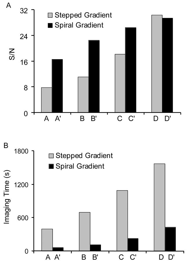
Plots of signal-to-noise ratio and imaging time for stepped gradients and spiral gradient data acquisition. A: The signal-to-noise ratio of the reconstructed images. The signal-to-noise ratio (SNR) was defined as the mean of the signal (>10% of the maximum signal intensity) divided by the standard deviation of the noise (<10% of the maximum signal intensity but greater than 0). The calculated SNR is 7.7, 10.9, 18.1, 30.2, 16.5, 22.4, 26.4 and 29.3. B: Imaging time. The imaging time for images A-D and A’-D’ is 392, 696, 1088, 1567, 58, 111, 223 and 428 s, respectively.
DISCUSSION
The quality of EPR images can be evaluated by the signal-to-noise ratio, the spatial resolution and the imaging time. There is always a trade-off among these three parameters: gaining in one means compromising on the other. For example, shorter imaging time can be achieved in conventional EPRI utilizing stepped gradient acquisition by either acquiring a smaller number of projections (lower spatial resolution) or by reducing the field sweep time (lower SNR), or both. However, the imaging speed in the stepped gradient data acquisition is also limited by the long hardware response time, given the number of projections to acquire. For example, with the L-band imaging system, the shortest imaging time was 392 s when 144 projections were acquired (See Fig. 4A). The spiral magnetic field gradient technique, on the other hand, has the great advantage of enabling much further reduction of the imaging time. In principle, the imaging time can be reduced to the fundamental limit imposed by the signal-to-noise ratio of the measurements, assuming that the gradient coils have a low inductance and sufficiently rapid response time. With the current trityl phantom, we have demonstrated good quality 3D images could be achieved in less than 2 minutes using spiral magnetic field gradient. The imaging time could be further reduced in higher signal-to-noise ratio cases, which can be made possible by increasing the concentration of the spin probe or using higher microwave power. In lower signal-to-noise ratio cases such as in in vivo experiments, less acceleration should be expected but the spiral approach is still useful in decreasing the star artifacts by acquiring more projections. Similar fast imaging techniques by rotating gradients have been well established in other imaging modalities such as spiral echo planar imaging (EPI) (27) and spiral computerized tomography (CT) (28, 29). Therefore, it is very intuitive to develop fast EPRI systems using spiral magnetic field gradient, in order to achieve a full range of trading imaging time with image quality.
The spiral magnetic field gradient technique enables acquisition of an unlimited number of projections in one field sweep of the main magnet. This feature is specially favorable to the back-projection based image reconstruction algorithms. In the filtered back-projection image reconstruction algorithm, the streak artifacts (also called star artifacts) will dramatically increase and dominate the noise in the reconstructed images when insufficient projections are acquired (30), as shown in Fig. 4A. With the capability of acquiring an unlimited number of projections, the spiral magnetic field gradient technique is able to improve the image quality by reducing the streak artifacts. This advantage is clearly shown in Figs. 6 and 7, where the spiral images A’, B’, and C’ were acquired with shorter imaging time and higher SNR, as compared to the regular images A, B and C, respectively.
The modified one-stage image reconstruction algorithm was used to reconstruct the 3D EPR images in the experiments. The advantage is that it allows the direct image reconstruction from the acquired projections. As pointed out previously, the one-stage image reconstruction algorithm involves heavy computation and is one- to two-order of magnitude slower in reconstruction speed compared to the 2-step filtered back-projection image reconstruction algorithm (19). For example, the reconstruction time was about 10 minutes for image D’ (6683 projections) in Fig. 4 on a Pentium 4 computer with 3.0 GHz CPU frequency. This disadvantage could be minimized by using the latest PC with dual-core multiple processors. Alternatively, it is possible to re-distribute these projections through interpolation so that the 2-step filtered back-projection algorithm can be used for faster image reconstruction. Obviously, the projection interpolation will introduce extra errors to the reconstructed images. In addition, the phenomenon of over-sampling near the pole (see Fig. 1) still remains in the spiral data acquisition approach. However, the uniform sampling scheme (19) could be incorporated into the spiral magnetic field gradient data acquisition by carefully designing the gradient waveforms with variable spiral frequency f2 . Therefore, a further up to 30% saving of imaging time is possible.
CONCLUSION
We developed and implemented a fast 3D EPR imaging system at L-band using spiral magnetic field gradient. This system is capable of acquiring a 3D image with more than 480 projections within 58 seconds. Good image quality was obtained with acquisition times 4 to 7-fold faster than the conventional stepped gradient approach. This fast imaging technique has great potential for the in vivo and ex vivo imaging of free radicals.
Acknowledgments
This work was supported by NIH Grants EB00254, EB00890 and EB005004. We thank Dr. Ilirian Dhimitruka for providing the trityl probe and Dr. Murugesan Velayutham for preparing the phantom. We also thank Dr. Ildar Salikhov and Mr. Joshua Civiello for technical assistance and Mr. Rizwan Ahmad for helpful discussions.
Footnotes
Publisher's Disclaimer: This is a PDF file of an unedited manuscript that has been accepted for publication. As a service to our customers we are providing this early version of the manuscript. The manuscript will undergo copyediting, typesetting, and review of the resulting proof before it is published in its final citable form. Please note that during the production process errors may be discovered which could affect the content, and all legal disclaimers that apply to the journal pertain.
References
- 1.Berliner LJ, Fujii H. Magnetic resonance imaging of biological specimens by electron paramagnetic resonance of nitroxide spin labels. Science. 1985;227:517–519. doi: 10.1126/science.2981437. [DOI] [PubMed] [Google Scholar]
- 2.Eaton GR, Eaton SS, Ohno K. EPR imaging and in vivo EPR. CRC Press; Boca Raton: 1991. [Google Scholar]
- 3.Berliner LJ. Biological magnetic resonance. Vol. 18 Kluwer Academic/Plenum Publishers; New York: 2003. [Google Scholar]
- 4.Zweier JL, Kuppusamy P. Electron paramagnetic resonance measurements of free radicals in the intact beating heart: a technique for detection and characterization of free radicals in whole biological tissues. Proc Natl Acad Sci U S A. 1988;85:5703–5707. doi: 10.1073/pnas.85.15.5703. [DOI] [PMC free article] [PubMed] [Google Scholar]
- 5.Halpern HJ, Jaffe DR, Nguyen TD, Haraf DJ, Spencer DP, Bowman MK, Weichselbaum RR, Diamond AM. Measurement of bioreduction rates of cells with distinct responses to ionizing radiation and cisplatin. Biochim Biophys Acta. 1991;1093:121–124. doi: 10.1016/0167-4889(91)90112-b. [DOI] [PubMed] [Google Scholar]
- 6.Swartz HM, Walczak T. Developing in vivo EPR oximetry for clinical use. Adv Exp Med Biol. 1998;454:243–252. doi: 10.1007/978-1-4615-4863-8_29. [DOI] [PubMed] [Google Scholar]
- 7.Swartz HM, Dunn JF. Measurements of oxygen in tissues: overview and perspectives on methods. Adv Exp Med Biol. 2003;530:1–12. doi: 10.1007/978-1-4615-0075-9_1. [DOI] [PubMed] [Google Scholar]
- 8.Lurie DJ, Mader K. Monitoring drug delivery processes by EPR and related techniques--principles and applications. Adv Drug Deliv Rev. 2005;57:1171–1190. doi: 10.1016/j.addr.2005.01.023. [DOI] [PubMed] [Google Scholar]
- 9.Subramanian S, Mitchell JB, Krishna MC. Time-Domain Radio Frequency EPR Imaging. In: Berliner LJ, editor. In Vivo EPR (ESR) - Theory and Application. Kluwer Academic/Plenum Publishers; New York: 2003. pp. 153–197. [Google Scholar]
- 10.Yamada K, Murugesan R, Devasahayam N, Cook JA, Mitchell JB, Subramanian S, Krishna MC. Evaluation and comparison of pulsed and continuous wave radiofrequency electron paramagnetic resonance techniques for in vivo detection and imaging of free radicals. J Magn Reson. 2002;154:287–297. doi: 10.1006/jmre.2001.2487. [DOI] [PubMed] [Google Scholar]
- 11.Eaton GR, Eaton SS. ESR imaging. In: Poole CP, Farach HA, editors. Handbook of Electron Spin Resonance. AIP Press, Springer; New York: 1999. pp. 327–343. [Google Scholar]
- 12.Kuppusamy P, Chzhan M, Vij K, Shteynbuk M, Lefer DJ, Giannella E, Zweier JL. Three-dimensional spectral-spatial EPR imaging of free radicals in the heart: a technique for imaging tissue metabolism and oxygenation. Proc Natl Acad Sci U S A. 1994;91:3388–3392. doi: 10.1073/pnas.91.8.3388. [DOI] [PMC free article] [PubMed] [Google Scholar]
- 13.Kuppusamy P, Li H, Ilangovan G, Cardounel AJ, Zweier JL, Yamada K, Krishna MC, Mitchell JB. Noninvasive imaging of tumor redox status and its modification by tissue glutathione levels. Cancer Res. 2002;62:307–312. [PubMed] [Google Scholar]
- 14.Demsar F, Walczak T, Morse PD, II, Bacic G, Zolnai Z, Swartz HM. Detection of diffusion and distribution of oxygen by fast-scan EPR imaging. J Magn Reson. 1988;76:224–231. [Google Scholar]
- 15.Oikawa K, Ogata T, Togashi H, Yokoyama H, Ohya-Nishiguchi H, Kamada H. A 3D- and 4D-ESR imaging system for small animals. Appl Radiat Isot. 1996;47:1605–1609. doi: 10.1016/s0969-8043(96)00167-4. [DOI] [PubMed] [Google Scholar]
- 16.Ohno K, Watanabe M. Electron paramagnetic resonance imaging using magnetic-field-gradient spinning. J Magn Reson. 2000;143:274–279. doi: 10.1006/jmre.1999.2005. [DOI] [PubMed] [Google Scholar]
- 17.Deng Y, He G, Petryakov S, Kuppusamy P, Zweier JL. Fast EPR imaging at 300 MHz using spinning magnetic field gradients. J Magn Reson. 2004;168:220–227. doi: 10.1016/j.jmr.2004.02.012. [DOI] [PubMed] [Google Scholar]
- 18.Jain AK. Fundamentals of digital image processing. Prentice-Hall, Inc; Englewood Cliffs, New Jersey: 1989. [Google Scholar]
- 19.Deng Y, Kuppusamy P, Zweier JL. Progressive EPR imaging with adaptive projection acquisition. J Magn Reson. 2005;174:177–187. doi: 10.1016/j.jmr.2005.01.019. [DOI] [PMC free article] [PubMed] [Google Scholar]
- 20.Kuppusamy P, Chzhan M, Zweier JL. Development and optimization of three-dimensional spatial EPR imaging for biological organs and tissues. J Magn Reson B. 1995;106:122–130. doi: 10.1006/jmrb.1995.1022. [DOI] [PubMed] [Google Scholar]
- 21.Xia S, Villamena FA, Hadad CM, Kuppusamy P, Li Y, Zhu H, Zweier JL. Reactivity of molecular oxygen with ethoxycarbonyl derivatives of tetrathiatriarylmethyl radicals. J Org Chem. 2006;71:7268–7279. doi: 10.1021/jo0610560. [DOI] [PMC free article] [PubMed] [Google Scholar]
- 22.Hoult DI, Goldstein S, Caponiti J. Electromagnet for nuclear resonance imaging. Rev Sci Instrum. 1981;52 [Google Scholar]
- 23.He G, Shankar RA, Chzhan M, Samouilov A, Kuppusamy P, Zweier JL. Noninvasive measurement of anatomic structure and intraluminal oxygenation in the gastrointestinal tract of living mice with spatial and spectral EPR imaging. Proc Natl Acad Sci U S A. 1999;96:4586–4591. doi: 10.1073/pnas.96.8.4586. [DOI] [PMC free article] [PubMed] [Google Scholar]
- 24.Hoch MJR, Ewert U. Resolution in EPR imaging. In: Eaton GR, Eaton SS, Ohno K, editors. EPR imaging and In Vivo EPR. CRC Press, Inc; Boca Raton: 1991. pp. 153–159. [Google Scholar]
- 25.Blass WE, Halsey GW. Deconvolution of absorption spectra. Academic Press; New York: 1981. [Google Scholar]
- 26.Deng Y, He G, Kuppusamy P, Zweier JL. Deconvolution algorithm based on automatic cutoff frequency selection for EPR imaging. Magn Reson Med. 2003;50:444–448. doi: 10.1002/mrm.10533. [DOI] [PubMed] [Google Scholar]
- 27.Haacke EM. Magnetic resonance imaging : physical principles and sequence design. Wiley-Liss; New York: 1999. [Google Scholar]
- 28.Fishman EK, Jeffrey RB. Spiral CT: principles, techniques, and clinical applications. Lippincott-Raven; Philadelphia: 1998. [Google Scholar]
- 29.Bahner ML, Reith W, Zuna I, Engenhart-Cabillic R, van Kaick G. Spiral CT vs incremental CT: is spiral CT superior in imaging of the brain? Eur Radiol. 1998;8:416–420. doi: 10.1007/s003300050403. [DOI] [PubMed] [Google Scholar]
- 30.Tseitlin M, Dhami A, Eaton SS, Eaton GR. Comparison of maximum entropy and filtered back-projection methods to reconstruct rapid-scan EPR images. J Magn Reson. 2006;184:157–168. doi: 10.1016/j.jmr.2006.09.027. [DOI] [PMC free article] [PubMed] [Google Scholar]