A Parametric Approach to Spectral-Spatial EPR Imaging

Abstract

Continuous wave electron paramagnetic resonance imaging for in vivo mapping of spin distribution and spectral shape requires rapid data acquisition. A spectral-spatial imaging technique is presented that provides an order of magnitude reduction in acquisition time, compared to iterative tomographic reprojection. The proposed approach assumes that spectral shapes in the sample are well-approximated by members from a parametric family of functions. A model is developed for the spectra measured with magnetic field modulation. Parameters defining the spin distribution and spectral shapes are then determined directly from the measurements using maximum a posteriori probability estimation. The approach does not suffer approximation error from limited sweep width of the main magnetic field and explicitly incorporates the variability in signal-to-noise ratio versus strength of magnetic field gradient. The processing technique is experimentally demonstrated on a one- dimensional phantom containing a nitroxide spin label with constant g-factor. Using an L-band EPR spectrometer, spectral shapes and spin distribution are accurately recovered from two projections and a spectral window which is comparable to the maximum linewidth of the sample.

1 Introduction

Electron paramagnetic resonance imaging (EPRI) is a noninvasive technique capable of mapping unpaired electrons for both endogenous and introduced free radicals [1,2]. The technique has evolved over two decades to become an important tool for studying free radicals in many branches of science [3–5] and has potential for the study of living biological systems [6–9]. Despite progress, high-quality EPR imaging has been limited by several technical factors including resolution, sensitivity, and acquisition time [10,11].

Spatial EPRI is capable of mapping the distribution of free radicals under the assumption that spectral lineshape is invariant throughout the object. Thus, for samples having spatially varying linewidths, or multiple radical species, accurate mapping of spin distribution is not possible using spatial EPRI. More importantly, spatial imaging only quantifies the spin content, providing no information about the nature of spins. To overcome this limitation, an additional dimension, the spectral dimension, is required to express spatially variant line-shape [12]. The imaging technique that includes a spectral dimension is termed spectral-spatial imaging. An example application of spectral-spectral EPRI is oximetry based on linewidth broadening from Heisenberg spin exchange interaction between a paramagnetic EPR spin probe and unpaired electrons in molecular oxygen [13].

In continuous wave (CW) EPRI, data is collected in the form of projections [14] which are acquired by measuring the absorption signal as a function of magnetic field in the presence of a static gradient. The strength and the orientation of the gradient vector are varied from projection to projection to encode the spectral and spatial information of the spins. Once an adequate number of projections are acquired, an image can be reconstructed using filtered backprojection (FBP) [15], which is based on the direct inversion of the Radon transform. To image the spectral dimension, projections are acquired at different gradient strengths. However, low signal-to-noise ratio (SNR), long acquisition time, and hardware limitations restrict the data acquisition at high gradient strengths. As a result, FBP imaging is degraded by the unobservable projections - a problem typically referred to as \missing angle tomography". The common solution is a projection-reprojection approach [16–18], in which missing data are synthesized at each iteration by computing projections through a FBP image or algebraic reconstruction image after smoothing the spectral dimension by curve fitting to an assumed lineshape function. The FBP or algebraic image reconstruction at each iteration requires a magnetic field sweep width that is several times the maximum linewidth to avoid error in truncating lineshape tails; a factor of 5 to 20 is typically adopted [19].

Thus, existing spectral-spatial imaging techniques are hampered by long collection times due to large sweep widths, large number of projections and by missing projection angles. In this work, we explicitly use prior knowledge of the lineshape functional form, such as Lorentzian, to address these deficiencies. Spectral-spatial EPR measurements are modeled as a function of spin density and lineshape parameters at each spatial location. Object properties are inferred from the data by maximum a posteriori probability (MAP) estimation. With no reliance on backprojection for inversion, the approach suffers no artifacts from missing projection angles, arbitrarily spaced sampling of gradient strength or spectral truncation. The estimation framework directly accounts for the decrease in SNR versus gradient strength, provides a principled means of selecting gradient strengths for acquisition, and reports noise sensitivity of estimated parameters. Simulation and experimental results demonstrate that reliable reconstruction is possible from two projections and a spectral window that is only equal to the maximum spectral linewidth. Additional projections or increased sweep width provide increased robustness to measurement noise. The proposed technique is described for two-dimensional spectral-spatial imaging and can be extended to higher dimensions.

2 Data Model

In this section, a mathematical model is formulated to describe the spectral-spatial EPR measurements in terms of the unknown spin density and spectral profile. For clarity and simplicity of presentation, one spatial dimension is considered here.

2.1 Parametric Object Model

Let the spatial dimension be denoted by y. The field of view (FOV) L is discretely approximated as K uniformly spaced piece-wise constant intervals numbered by k from −K/2 to K/2 −1. For interval k, the lower and upper endpoints y_l,k and y_u,k are given by

$$y_{l,k}=k\frac{L}{K}\hspace{0.17em}\text{and\hspace{0.17em}}{y}_{u,k}=(k+1)\frac{L}{K}$$ (1)

On each interval, the spectral dimension, denoted by h, is assumed to have a Lorentzian lineshape. The spin density and Lorentzian half-linewidth (i.e., half width at half maximum) in the k^th interval are denoted by d_k and τ_k, respectively. The center of the Lorentzian is assumed to be known, constant, and equal to h₀ for every interval. Thus, the spectral-spatial object model is given by

$$S(y,h)=\frac{d_k{\tau }_k}{{(h-h_0)}^2+{\tau }_k^2},\hspace{0.17em}\hspace{0.17em}\hspace{0.17em}{y}_{l,k}\le y<y_{u,k}$$ (2)

Let d and τ denote the lists of K spin densities and K half-linewidths specifying the object model, and define ξ = [dτ]^Τ to be the column vector of the 2K parameters.

2.2 Parametric Projection Model

The geometry of a 2D spectral-spatial projection is depicted in Fig. 1. A static gradient field is used to create a pseudo angle α, where $\frac{\sqrt{2}\mathrm{\Delta }H}{cos\alpha }$ is the sweep-width and ΔH is the spectral window; the maximum pseudo angle α_max relates to the physical maximum gradient G_max by L = tan(α_max)ΔH=G_max [20].

Fig. 1.

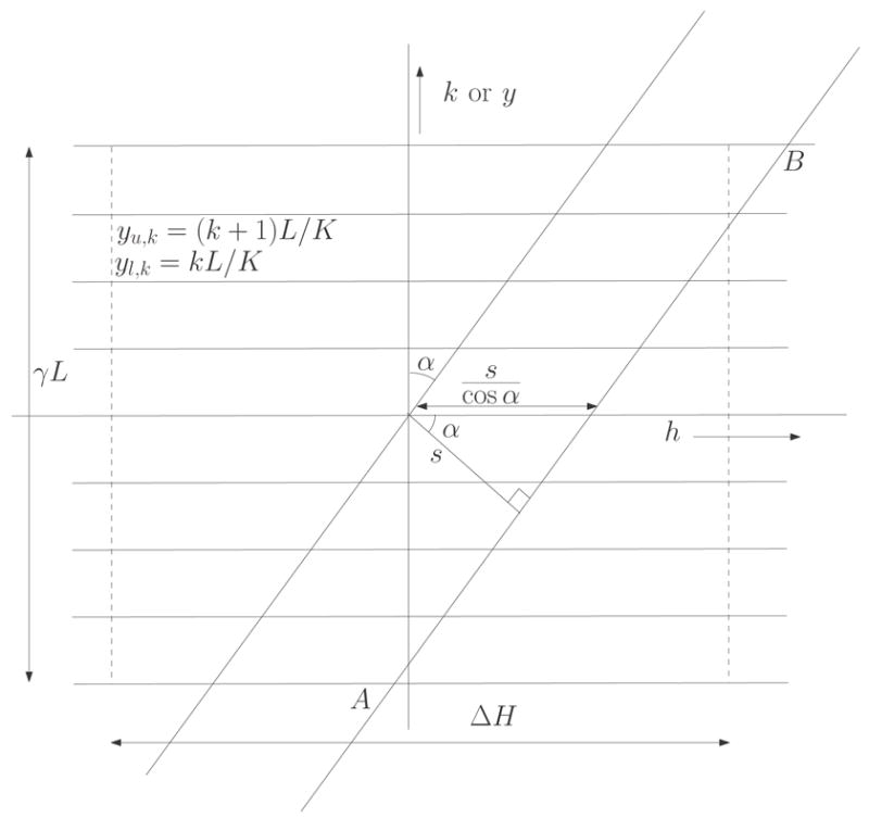
In spectral-spatial imaging, line integrals are measured through a pseudo object by first applying a static magnetic field gradient, then sweeping the main (uniform) magnetic field to excite electron magnetic moments. Here, the vertical axis is the spatial axis and the horizontal axis is the spectral axis. The spatial axis is normalized to make the FOV same as the spectral window ΔH; γ = ΔH/L is the normalizing constant.

The normal distance of the line of integration from the origin of the pseudo object is denoted by s. The line of projection (AB) is given by

$$h=y\frac{\mathrm{\Delta }H}{L}tan\alpha +\frac{s}{cos\alpha }$$ (3)

and intersects the lower and upper edges of the k^th segment at positions y_l;k and y_u,k, respectively. The corresponding h co-ordinates are

$$h_{l,k}(s,\alpha )=y_{l,k}\frac{\mathrm{\Delta }H}{L}tan\alpha +\frac{s}{cos\alpha }$$ (4)

$$h_{u,k}(s,\alpha )=y_{u,k}\frac{\mathrm{\Delta }H}{L}tan\alpha +\frac{s}{cos\alpha }$$ (5)

The projection P(s, α, ξ) is given by the line integral

$$P(s,\alpha ;\underset{\_}{\xi })=\frac{c}{sin\alpha }\sum _{k=-\frac{K}{2}}^{\frac{K}{2}-1}\underset{h_{l,k}(s,\alpha )}{\overset{h_{u,k}(s,\alpha )}{\int }}\frac{d_k{\tau }_k}{{(h-h_0)}^2+{\tau }_k^2}dh$$ (6)

where c is a calibration constant. Note that the projection lines are not truncated by any spectral window; therefore, the model does not suffer the approximation error introduced in inverse Radon transform reconstruction by neglecting contribution from area under the tails of the spectral lineshape outside the spectral window.

If the modulation amplitude and frequency are small, then the measured data f(s, α; ξ) due to Zeeman modulation are proportional to the the first derivative of P(s, α; ξ) with respect to s and are scaled by a factor of cos²α [19].

$$\begin{array}{l}f(s,\alpha ;\underset{\_}{\xi })=\stackrel{\sim }{c}({cos}^2\alpha )\frac{\partial }{\partial s}P(s,\alpha ;\underset{\_}{\xi })=\stackrel{\sim }{c}\sum _{k=-\frac{K}{2}}^{\frac{K}{2}-1}\frac{d_k{\tau }_k}{tan\alpha }\\ \times \left(\frac{1}{{(h_{u,k}(s,\alpha )-h_0)}^2+{\tau }_k^2}-\frac{1}{{(h_{l,k}(s,\alpha )-h_0)}^2+{\tau }_k^2}\right)\end{array}$$ (7)

where c̃ is the revised calibration constant.

If N samples are taken at every angle, then s may be replaced by sample number n in Eq. [7] using

$$s=\frac{\sqrt{2}\mathrm{\Delta }Hn}{N},\hspace{0.17em}\hspace{0.17em}\hspace{0.17em}n=-N/2,\dots ,N/2-1$$ (8)

Substitution of eqns. (1) and (8) into eqns. (7), (4) and (5) yields

$$\begin{array}{l}f(n,\alpha ;\underset{\_}{\xi })=\frac{\stackrel{\sim }{c}}{tan\alpha }\sum _{k=-\frac{K}{2}}^{\frac{K}{2}-1}{d}_k{\tau }_k\\ \times \left(\frac{1}{{(h_{u,k}(n,\alpha )-h_0)}^2+{\tau }_k^2}-\frac{1}{{(h_{l,k}(n,\alpha )-h_0)}^2+{\tau }_k^2}\right)\\ h_{l,k}(n,\alpha )=k\frac{\mathrm{\Delta }H}{K}tan\alpha +\frac{\sqrt{2}\mathrm{\Delta }Hn}{Ncos\alpha }\\ h_{u,k}(n,\alpha )=(k+1)\frac{\mathrm{\Delta }H}{K}tan\alpha +\frac{\sqrt{2}\mathrm{\Delta }Hn}{Ncos\alpha }\end{array}$$ (9)

Note that by application of L'Hôpital's rule to Eq. [9], the zero gradient projection case, i.e.,α = 0, gives

$$f(n,0;\underset{\_}{\xi })=\frac{2\stackrel{\sim }{c}\mathrm{\Delta }H}{K}\sum _{k=-\frac{K}{2}}^{\frac{K}{2}-1}\frac{d_k{\tau }_k\left(h_0-\frac{\sqrt{2}\mathrm{\Delta }Hn}{N}\right)}{{\left({(\frac{\sqrt{2}\mathrm{\Delta }Hn}{N}-h_0)}^2+{\tau }_k^2\right)}^2}$$ (10)

2.3 Noise Model

Measurement noise is modeled as additive, zero mean, Gaussian, and uncorrelated with variance σ². Let Y denote the measurements, with samples from all angles concatenated. Thus, Y is a multi-variate Gaussian random vector with mean f and diagonal covariance matrix σ²I.

Given this parametric model, spectral-spatial imaging is the task of inferring parameters d and τ from the noisy observations, Y.

3 Parameter Estimation

A Bayesian approach is adopted for parameter estimation and yields a regularized least-squares inversion. A confidence measure for estimated parameters is determined using the Cramμer-Rao lower bound.

3.1 Maximum A Posteriori Probability (MAP) Estimate

The parameter vector ξ is estimated by maximizing the posterior probability of ξ given the noisy measurements, Y [23]. Invoking Bayes' formula,

$$\begin{array}{l}\underset{\_}{\widehat{\xi }}=arg\underset{\underset{\_}{\xi }}{max}p(\underset{\_}{\xi }\mid \underset{\_}{\mathbf{Y}})=arg\underset{\underset{\_}{\xi }}{max}\frac{p(\underset{\_}{\mathbf{Y}}\mid \xi )p(\underset{\_}{\xi })}{p(\underset{\_}{\mathbf{Y}})}\\ =arg\underset{\underset{\_}{\xi }}{min}-\left\{logp(\underset{\_}{\mathbf{Y}}\mid \underset{\_}{\xi })+logp(\underset{\_}{\xi })\right\}\\ =arg\underset{\underset{\_}{\xi }}{min}\frac{1}{2{\sigma }^2}\sum _{n,\alpha }{\left(Y(n,\alpha )-f(n,\alpha ;\underset{\_}{\xi })\right)}^2+g(\underset{\_}{\xi })\end{array}$$ (11)

The prior probability density p(ξ) ∝ exp{−g(ξ)} is used to encode prior knowledge of the spectral-spatial object. We adopt

$$g(\underset{\_}{\xi })=\sum _{k=-K/2}^{K/2-2}{\lambda }_d{(d_{k+1}-d_k)}^2+{\lambda }_{\tau }{({\tau }_{k+1}-{\tau }_k)}^2$$ (12)

to express the belief that smooth distributions of spin density and half-linewidth are likely.

For decreasing (λ_d, λ_τ) and fixed measurement noise power σ², the MAP estimate allows less smoothness and enforces greater fidelity to the noisy measurements. Here, we adopt 2σ²λ_τ = 2σ²λ_d = λ, assuming the dynamic range of numerical magnitudes of d_k and τ_k to be of the same order; this can be achieved either by choosing appropriate units of d_k and τ_k or by scaling dk and absorbing the scaling factor into c̃. Multiplying the cost function of Eq. [11] by 2σ² yields

$$\begin{array}{l}\underset{\_}{\widehat{\xi }}=arg\underset{\underset{\_}{\xi }}{min}\sum _{n,\alpha }{\left(Y(n,\alpha )-f(n,\alpha ;\underset{\_}{\xi })\right)}^2\\ +\lambda \sum _{k=-K/2}^{K/2-2}{(d_{k+1}-d_k)}^2+{({\tau }_{k+1}-{\tau }_k)}^2\end{array}$$ (13)

The function g(ξ) alternatively may be viewed as a regularization term added to the least-squares cost. Roughness penalties are commonly adopted for image reconstruction and restoration to combat oscillation in least-squares solutions: see, e.g., [21,22] and references therein.

3.2 Numerical optimization

The optimization task in Eq. [13] may be solved by many numerical methods; we use the interior-reflective Newton method implemented in the Matlab ¹ 7.1 routine lsqnonlin. Note that the cost function is quadratic in d but non-convex in τ. Further, the gradient of the cost function is easily computed. The iterative optimization algorithm is initialized at d_k = 0 and τ_k = τ_min for each k, where τ_min > 0 is a minimum physically meaningful half-linewidth. In addition, the spin density is constrained by d_k ≥ 0 and half-linewidth by τ_min ≤ τ_k ≤ τ_max.

3.3 Cramér-Rao Bound on Error Variance

The Cramér-Rao bound (CRB) gives a lower bound on the parameter estimation error variance for any unbiased estimator [23]. We use the CRB to calculate the posterior confidence interval for estimated parameters. The bound is obtained by inverting the Fisher information matrix, I_F

$$\mathbf{E}\left[(\underset{\_}{\widehat{\xi }}-\underset{\_}{\xi }){(\underset{\_}{\widehat{\xi }}-\underset{\_}{\xi })}^T\right]\ge {{\mathbf{I}}_{\mathbf{F}}}^{-1}$$ (14)

where E denotes expectation, the left-hand side is the 2K-by-2K error covariance matrix, and the inequality A ≥ B denotes that the matrix difference A – B is non-negative definite.

In the Bayesian estimation framework, the Fisher information matrix I_F is the sum of two terms: I_M due to measurements and I_P from the prior information [23], where the (i; j)^th elements of I_M and I_P are given by

$${\mathbf{I}}_{\mathit{Mij}}=-\mathbf{E}\left[\frac{{\partial }^{2}lnp(\underset{\_}{\mathbf{Y}}\mid \underset{\_}{\xi })}{\partial {\xi }_i\partial {\xi }_j}\right]$$ (15)

and

$${\mathbf{I}}_{\mathit{Pij}}=-\mathbf{E}\left[\frac{{\partial }^{2}lnp(\underset{\_}{\xi })}{\partial {\xi }_i\partial {\xi }_j}\right]$$ (16)

Fisher information describes the local curvature of the log-likelihood function and admits an intutive interpretation. At parameter values for which the log-likelihood has low curvature (i.e., is relatively flat), the cost function in Eq. [13] is not sensitive to small changes in the estimated parameters; hence, the estimation error variance due to measurement noise is relatively large. In contrast, where the log-likelihood function has high curvature, the cost is sensitive to small changes in the estimated parameters, resulting in low variance parameter estimates.

In section 5, the proposed imaging procedure is applied to measured data collected from nitroxide solutions using an L-band spectrometer. As prelude, section 4 explores two questions via computer simulation. First, what is the sensitivity of parameters to perturbations in measured data? Second, which projection angles are most informative?

4 Simulation Results

The data model postulated in section 2 and inversion procedure described in section 3 are examined via numerical simulations. Synthetic experiments are used to evaluate sensitivity to local minima, to quantify sensitivity to additive measurement noise, to study polynomial correction of baseline drift, to explore selection of projection angles, and to evaluate selection of regularization constant.

Simulation results are reported for the piece-wise constant phantom shown in Fig. 2. The Lorentzian peak location is h₀ = 1 G. For sections 4.1 and 4.2, the simulation parameters are: spectral window ΔH = 3 G, K = 32 spatial segments, N = 256 samples per projection angle and two projections at α = −83.1 ° and −69.2 °.

Fig. 2.

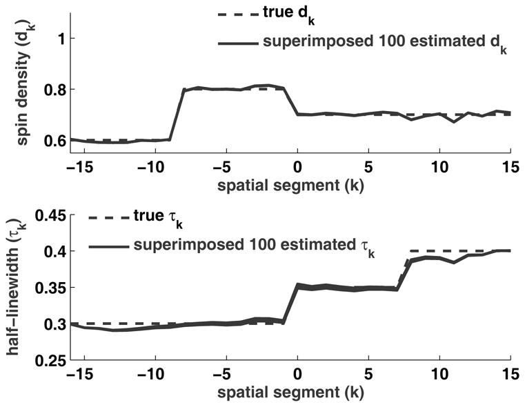
1D spatial phantom with K = 32 and piece-wise constant spin density and half-linewidth (dashed lines). Estimated d_k and τ_k (solid lines) from 100 random initializations and for a fixed noise realization at 30 dB (σ = 0.0051). The 100 estimated profiles are superimposed.

One goal in simulation is to evaluate the relative information content of different projection angles. Therefore, λ is set to zero to avoid any confounding influence from the smoothness prior, p(ξ).

4.1 Convexity and Initialization

Numerical experience suggests that local minima do not pose a hazard to the nonconvex optimization in Eq. [13]. To test sensitivity to initialization, the optimization routine was executed for 100 random initializations, d_k uniform on [0, 1] and τ_k uniform on [0:05, 0:9], k = −16,…, 15. Fig. 2 shows the superimposed estimated d_k and τ_k for 100 random initializations. The signal-to-noise ratio (SNR) was set at 30 dB, where SNR is defined as the ratio of signal power to noise power. The maximum, across all k and all trials, of observed variance of spin density (d_k) estimates is 3.3 × 10⁻⁷ and that of half-linewidth (τ_k) estimates is 8.5 × 10⁻⁷. The maximum, across k, of absolute deviation from the mean estimate for d_k is 0:0027 and for τ_k is 0:0044.

4.2 Bias and Variance

The spin density and half-linewidth were estimated from 500 different noise realizations. The mean estimation error for d_k has a maximum absolute value of 2.6 × 10⁻³ across k and the same for τ_k is 2.8 × 10⁻³ at 30 dB SNR. Thus, the mean estimation errors are negligible.

Fig. 3 displays simulated error standard deviation of half-linewidth (τ_k) from 500 different noise realizations, along with the corresponding Cramér-Rao bound. The figure illustrates the efficacy of the theoretical bound to characterize noise sensitivity. Two themes are seen which are likewise observed for other synthetic phantoms: uncertainty in lineshape increases for lower spin density, and uncertainty decreases away from the center of the FOV.

Fig. 3.

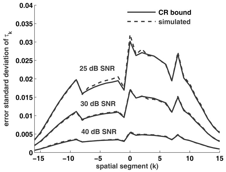
Theoretical bound and simulated (from 500 trials) error standard deviations for half-linewidths τ_k.

4.3 Angle Selection

The Cramer-Rao bound can also inform selection of projection angles. Fig. 4 shows the CRB for error standard deviation of the d₂ and τ₂ parameters versus angle of projection for the object shown in Fig. 2. The graphs illustrate the two opposing effects of higher gradient strengths. On one hand, higher gradient, hence higher projection angle, yields more informative projections. On the other hand, the higher gradient yields lower SNR. The two effects combine in Fig. 4 to give minimum parameter error at a high angle near 80 degrees. To explore a combination of projection angles, Fig. 5 displays the CRB for various pairs of angles and shows that (80, 60) is preferred over the nearly complementary angle pair (85, 5). This CRB sensitivity analysis can only be computed for a known object; nonetheless, it was observed that the error bounds for many objects show the same trends as found in Fig. 4 and Fig. 5. Thus studying the CRB for simulated objects can guide the selection of projection angles to be collected in practice.

Fig. 4.

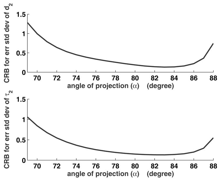
Cramér-Rao bound of the spin density d₂ and half-linewidth τ₂ versus angle of projection α.

Fig. 5.

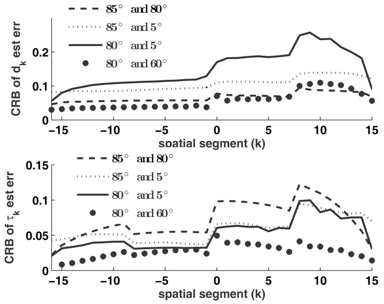
Cramér-Rao bound for the spin density d_k and half-linewidth τ_k for various combinations of angles of projection α.

4.4 Selection of Regularization Constant

To explore dependence of reconstruction error on the parameter λ, simulations were run at SNR values from 15 dB to 35 dB in 5 dB steps. Reconstructions were computed for λ in the set {0, 0.001, 0.001, 0.01, 0.1, 1}. The root mean square error (RMSE) was averaged from 50 trials at each combination of SNR and λ. Over the range of SNR values considered, selection of λ from the three orders of magnitude {0.001, 0.01, 0.1} yields similar RMSE; no more than 3.6% difference was observed. Thus a wide range of λ values is found to give similar reconstruction results.

With decreasing SNR, the RMSE increases; and the value of λ, yielding lowest RMSE is SNR dependent. The choice λ = 0.1 yielded lowest RMSE for SNR values of 20, 25 and 30 dB. Expectedly, at lower SNR, λ should be increased to reflect the reduced fidelity of the measured data.

4.5 Baseline Drift Correction

Since the sweep-width is of the order of linewidth of the Lorentzian, the standard baseline drift correction method on the measured data after integration cannot be applied directly in the proposed approach. Instead a polynomial model of the baseline is added to the forward projection model and the parameters of the polynomial at each projection angle are estimated from the measured data. Simulation showed that if a baseline drift of 20% of the output signal peak per Gauss is introduced, then the average RMSE of τ from 50 trials is 43% at 30 dB SNR when baseline drift in not included in the model. But if a baseline drift model is used, then the the average RMSE drops to 5%. Fig. 6 shows a typical reconstruction result from projections with baseline drift.

Fig. 6.

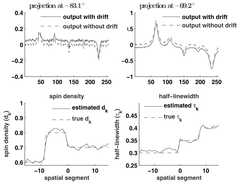
Projections with and without baseline drift and true and estimated parameters. The data with baseline drift were used for parameter estimation. A linear baseline correction model on the unmodulated projection was assumed and the same correction model gives a constant drift correction in the modulated projection model. At the −83.1 ° projection the drift is positive and at −69.2 ° projection the drift is negative. The SNR value is 25 dB and the regularization constant λ = 0.1.

5 Experimental Results

An experiment was performed to validate the proposed technique and its performance. Lineshape is characterized, spin density and half-linewidth are estimated from measured data, the residual between measured data and model fit is analysed, and Cramér-Rao bounds are reported.

The phantom shown in Fig. 7 was constructed from three tubes with inner diameter of 2.75 mm each and outer diameter of 4.0 mm. Tubes were filled with three different concentrations (1.0, 0.8, and 0.5 mM from left to right) of ¹⁵ N-PDT (4-Oxo-2,2,6,6-tetramethyl-piperidine-d₁₆-¹⁵N-oxy) radical dissolved in distilled water. Chromium oxalate (CrOx) in distilled water was used as a broadening agent. The concentrations of CrOx in the three solutions were 0, 2.33 and 0.65 mM respectively. A detailed discussion on CrOx induced linebroadening is given elsewhere [24].

Fig. 7.

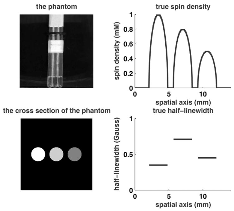
The phantom used for experiment. Top-left: Photograph of the phantom; the three tubes are glued together and filled with nitroxide solutions with three different concentrations mixed with different amounts of the broadening agent. Bottom-left: Schematic of the cross-section of the inner perimeters of the tubes. The magnetic field gradient is along the horizontal axis. Top-right: Spin density profile. Bottom-right: Half-linewidth profile.

5.1 Lineshape Characterization

To charcterize the lineshape function, the absorption signal from each tube was measured separately using an L-band (1.2 GHz) EPR spectrometer. The Lorentzian curve-fit for the 0.5 mM solution is shown in Fig. 8. The results of curve-fit for all three solutions are summarized in Table 1. The fit error is defined as the ratio of the norm of residual to the norm of measured lineshape.

Fig. 8.

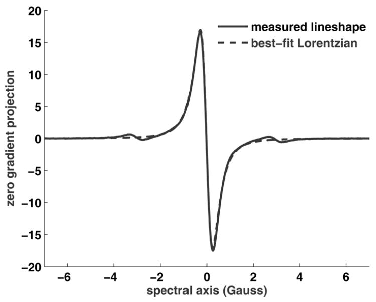
Measured zero gradient projection of the 0.5 mM solution and the best-fit Lorentzian. The fit error is 5.2%.

Table 1.

Characterization results of solutions used in the phantom. The spin densities in the three tubes are proportional to the solution strengths. The half-linewidths are obtained from Lorentzian curve-fit to the zero gradient projections obtained for the three solutions.

Concentrations	% fit err	fit err (dB)	τ (Gauss)
1.0 mM	5.2%	−25.7 dB	0.35
0.8 mM	4.7%	−26.5 dB	0.71
0.5 mM	5.2%	−25.7 dB	0.45

5.2 Spectral-spatial Imaging

Imaging was carried out with a reentrant resonator of diameter of 12.6 mm and a useable height of 12 mm. Results are reported in sections 5.3, 5.4 and 5.5 for the following spectrometer settings: incident power 4 mW; spectral window ΔH = 1.4 G; spatial field of view L = 14.14 mm; modulation amplitude 0.2 G; modulation frequency 100 kHz. Various spectrometer settings gave consistent reconstruction results. A total of 13 projections were acquired. Each acquired projection had 4096 data points which were downsampled to 256 points. No corrections for baseline or B1 field inhomogeneities [25] were applied.

5.3 Parameter Estimation

Spin density and half-linewidth are estimated using Eq. [13], and the reconstructed object is shown in Fig. 9, the estimated spin density and estimated half-linewidth are shown in the Fig. 10. Two angles of projection, −83.1 ° (8.3 G/cm) and −69.2 ° (2.6 G/cm), are used, and the proportionality constant c̃ is chosen so that the spin densities d_k have approximately the same range of values as the half-linewidths τ_k. The modulation gave a measured PSNR of 14.4 in the −83.1 ° projection and 63.6 for the −69.2 ° projection, where PSNR is the ratio of the peak signal to the peak noise. The total acquisition time for these two projection angles is 59.3 s. In the numerical optimization, λ = 0.01, τ_min = 0.3 G and τ_max = 0:9 G. The computation time is 4.14 s 4.46 s on a Pentium^® D 2.6 GHz processor with 2 GB RAM.

Fig. 9.

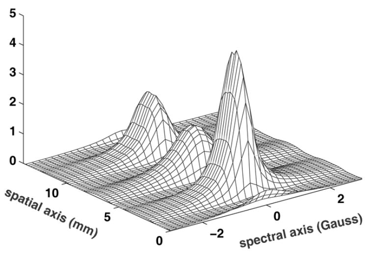
Reconstructed spectral-spatial object from experimental data. Two angles of projections at −83.1 ° and −69.2 °, with 256 samples at each angle, are used. The regularization coefficient is λ = 0.01. The spectral window, ΔH, is 1.4 G, and the maximum linewidth of the Lorentzian present is 1.4 G.

Fig. 10.

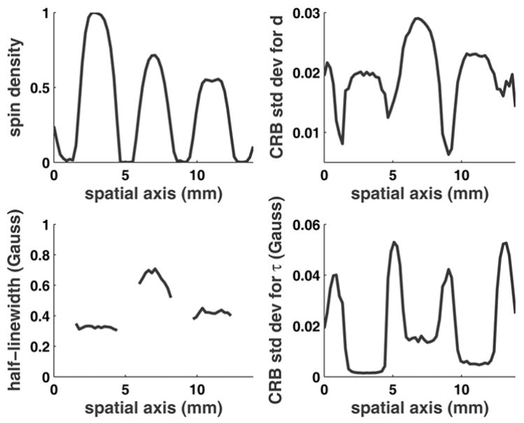
Top-left: Reconstructed spin density (d_k) values from experimental data. Bottom-left: Reconstructed half-linewidth (τ_k) values. Top-right: Cramér-Rao bounds for estimation error standard deviations of d_k. Bottom-right: Cramér-Rao bounds for estimation error standard deviations of τ_k. The d_k and τ_k estimates are accepted if the CRB is less than 10 times the minimum of CRB across all k, otherwise they are discarded and not shown in the left column d_k and τ_k plots.

5.4 Residual Analysis

The noise assumptions are examined by analysis of the residual. The residual, Y (n, α) – f(n, α ξ), is the fit error between the measured data and the estimated parametric model in Eq. [9]. Fig. 11 shows the measured projection and the fit error. The observed signal-to-noise ratio is 32.5 dB. A Lilliefors test, with 0.05 level of significance, accepts the hypothesized Gaussian distribution, p = 0.15.

Fig. 11.

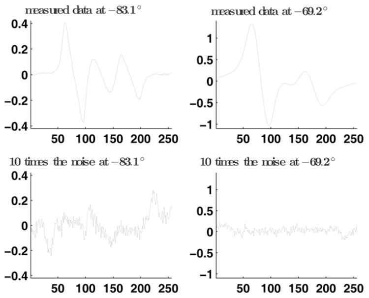
Measured data and residual fit error. Top-left: The measured data at −83.1 °. Top-right: Measured data at −69.2 °. Bottom-left: 10 times the residual fit error at −83.1 °. Bottom-right: 10 times the residual fit error at −69.2 °. The vertical axis is in arbitraty unit and the horizontal axis denotes sample number.

5.5 Cramér-Rao Bound

Cramér-Rao bounds for estimation error standard deviations of d_k and τ_k are computed using ξ̲̂ and σ̂², where ξ̲̂ is the estimated parameter vector and σ̂² is the measured variance of the residual. The bounds are shown in Fig. 10. The standard deviation of τ_k estimation error is high between the tubes where there is no spin density. If the error standard deviation is less than 10 times the minimum of CRB across all k, then the estimated values are accepted and are otherwise discarded. Note that this reliability analysis shows only the effect of additive measurement noise and does not take into account the effects of magnetic field inhomogeneity or error introduced by deviation of lineshapes from the functional form in Eq. [2].

6 Comparison with Projection-reprojection Method

Performance of a projection-reprojection method [16] was analysed using a simulated tube phantom similar to the one used for the experiment. The use of simulation was necessitated by the inability of our spectrometer to measure the wide sweep width required to follow the published guidelines suggested for projection-reprojection. Fig. 12 shows the reconstruction results from the projection-reprojection and parametric approaches. For the parametric method the spectral window and projection angles reported in section 5 were again used. With simulated noise of 30 dB SNR the reconstruction error for τ was 5.4% using the two projection angles and λ = 0. The corresponding data acquisition time is 59.3 s, assuming a sweep rate of 0.19 G/s and a main field recovery time of 1 sec.

Fig. 12.

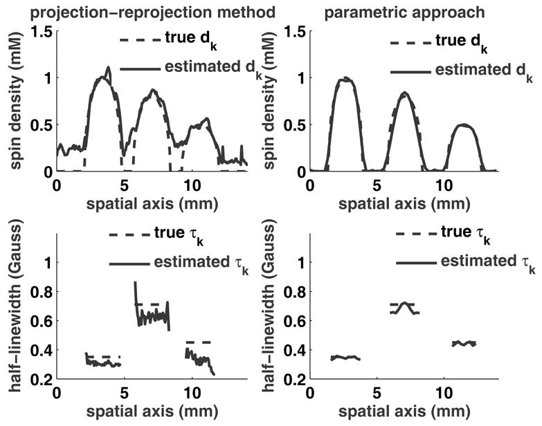
Reconstructed spin density and half-linewidth by projection-reprojection and parametric methods.

For the projection-reprojection method, the data acquisition and algorithm parameters were varied in an attempt to obtain the lowest reconstruction error with the least acquisition time. The spectral window was 14.1 times the maximum linewidth present; 15 projection angles were used, uniformly spaced from −81 ° to 81 °. An additional 16 angles were used for reprojection, 14 of which were selected at the mid-points between the measured angles, and −85.5 ° and 85.5 ° angles were selected at the high gradient region. The PSNR for the zero gradient projection was equivalent for the two methods. The reconstruction error for τ after six iterations was 18.6%. The corresponding data acquisition time for the reprojection imaging is 37.83 min.

Thus, for this phantom the parametric approach required 38 times less data acquisition time compared to the projection-reprojection method and yielded lower reconstruction error.

7 Discussion

The proposed parametric estimation approach offers significant reduction in data acquisition time for spectral-spatial EPR imaging. The savings come from both a small spectral window and a low number of projections. In comparison to tomographic reprojection methods for the examples considered, the reduced sweep width and reduced number of projections combine to yield 30 : 1 to 40 : 1 reduction in data acquisition time for equal or lower reconstruction error.

The maximum a posteriori probability estimation approach adopted in Eq. [13] reduces to maximum likelihood (ML) estimation for regularization parameter λ = 0. For Gaussian noise, the ML estimate is the nonlinear least squares curve fit. A nonzero λ reduces the oscillatory artifacts seen in a least squares solution. The estimation procedure is not sensitive to the choice of λ; for the experimental data in Section 5, values of λ across three orders of magnitude, 0.01 ≤ λ ≤ 1, give similar reconstruction results.

Higher error at the center of the FOV is observed in both simulation and measurement. Physically, consider the line integrals through the pseudo-object that yield the samples near either end of a projection. These line integrals depend on only a few spatial locations, and therefore have contribution from only a few unknown values of spin density and line width. Consequently, parameters at the ends of the 1D spatial object are less sensitive to estimation error.

The proposed imaging approach is a direct inversion of the measured data using a regularized nonlinear regression. Unlike tomographic approaches, no approximation error is introduced by truncation of the lineshape by the spectral window. The estimation procedure is applicable for any set of arbitrarily spaced projection angles and is not handicapped by the missing angle artifact introduced by tomographic inversion. Additionally, the estimation approach directly and explicitly incorporates into the inversion the noise properties of the spectral-spatial measurements. In contrast, in tomographic processing with magnetic field modulation, numerical integration to obtain projection data introduces strong noise correlation, and backprojection disregards the high variability in PSNR that is due to the cos²α scaling shown in Eq. [7].

The model-based inversion exploits prior knowledge that the spectral line-shapes are from a parametric family of functions. Using the model in Eq. [2], the number of unknowns in a K × K image is reduced from K² to 2K. Moreover, as illustrated in Fig. 1, every sample from each projection angle contains information from every spatial location, thereby permitting recovery of the spin density and linewidth from a single projection in the noiseless case. Additional projections provide increased robustness to measurement noise and modeling imperfections.

The proposed imaging procedure given by Eq. [13] may be readily extended in two ways. First, extension to three spatial dimensions requires no new assumptions and entails only modification of Eq. [6] to compute a definite integral over the surface of a planar slice through a voxel. Second, the lineshape model in Eq. [2] may be extended from Lorentzian to any parametric function, such as a mixture of Lorentzians with unknown central locations, or the convolution of a Gaussian with a Lorentzian.

A strength of the proposed processing procedure is the explicit identification of the physical assumptions adopted in its derivation. This transparency allows informed judgment concerning the suitability of the technique for any candidate application.

8 Conclusion

We have presented a parameter estimation framework for spectral-spatial EPR imaging. The approach provides reliable reconstruction of spin density and spectral linewidth with an order of magnitude reduction in data acquisition time, compared to tomographic inversion. The proposed technique is suitable for any application in which spectral lineshapes under study can be accurately approximated as members of a parametric family of functions. The imaging procedure was demonstrated using computer simulation and measurements on an experimental phantom.

References

- 1.Fujii H, Berliner LJ. One- and two-dimensional EPR imaging studies on phantoms and plant specimens. Magn Reson Med. 1985;2:275–282. doi: 10.1002/mrm.1910020310. [DOI] [PubMed] [Google Scholar]
- 2.Ferrari M, Quaresima V, Sotgiu A. Present status of electron paramagnetic resonance (EPR) spectroscopy/imaging for free radical detection. Pflugers Arch. 1996;431:R267–268. doi: 10.1007/BF02346371. [DOI] [PubMed] [Google Scholar]
- 3.Fuchs J, Freisleben HJ, Groth N, Herrling T, Zimmer G, Milbradt R, Packer L. One- and two-dimensional electron paramagnetic resonance imaging in skin. Free Radic Res Commun. 1991;15:245–253. doi: 10.3109/10715769109105220. [DOI] [PubMed] [Google Scholar]
- 4.Hochi A, Furusawa M, Ikeya M. Applications of microwave scanning ESR microscope: human tooth with metal. Appl Radiat Isot. 1993;44:401–405. doi: 10.1016/0969-8043(93)90256-a. [DOI] [PubMed] [Google Scholar]
- 5.Kuppusamy P. EPR spectroscopy in biology and medicine. Antioxid Redox Signal. 2004;6:583–585. doi: 10.1089/152308604773934332. [DOI] [PubMed] [Google Scholar]
- 6.Kuppusamy P, Shankar RA, Roubaud VM, Zweier JL. Whole body detection and imaging of nitric oxide generation in mice following cardiopulmonary arrest: detection of intrinsic nitrosoheme complexes. Magn Reson Med. 2001;45:700–707. doi: 10.1002/mrm.1093. [DOI] [PubMed] [Google Scholar]
- 7.Matsumoto A, Matsumoto S, Sowers AL, Koscielniak JW, Trigg NJ, Kuppusamy P, Mitchell JB, Subramanian S, Krishna MC, Matsumoto K. Absolute oxygen tension (pO2) in murine fatty and muscle tissue as determined by EPR. Magn Reson Med. 2005;54:1530–1535. doi: 10.1002/mrm.20714. [DOI] [PubMed] [Google Scholar]
- 8.Rolett EL, Azzawi A, Liu KJ, Yongbi MN, Swartz HM, Dunn JF. Critical oxygen tension in rat brain: a combined (31)P-NMR and EPR oximetry study. Am J Physiol Regul Integr Comp Physiol. 2000;279:R9–R16. doi: 10.1152/ajpregu.2000.279.1.R9. [DOI] [PubMed] [Google Scholar]
- 9.Velayutham M, Li H, Kuppusamy P, Zweier JL. Mapping ischemic risk region and necrosis in the isolated heart using EPR imaging. Magn Reson Med. 2003;49:1181–7. doi: 10.1002/mrm.10473. [DOI] [PubMed] [Google Scholar]
- 10.Deng Y, He G, Petryakov S, Kuppusamy P, Zweier JL. Fast EPR imaging at 300 MHz using spinning magnetic field gradients. J Magn Reson. 2004;168:220–227. doi: 10.1016/j.jmr.2004.02.012. [DOI] [PubMed] [Google Scholar]
- 11.Joshi JP, Ballard JR, Rinard GA, Quine RW, Eaton SS, Eaton GR. Rapid-scan EPR with triangular scans and fourier deconvolution to recover the slow-scan spectrum. J Magn Reson. 2005;175:44–51. doi: 10.1016/j.jmr.2005.03.013. [DOI] [PubMed] [Google Scholar]
- 12.Maltempo MM, Eaton SS, Eaton GR. Spectral-spatial two-dimensional EPR imaging. J Magn Reson. 1987;72:449–455. [Google Scholar]
- 13.Halpern HJ, Yu C, Peric M, Barth E, Grdina DJ, Teicher BA. Oxymetry deep in tissues with low frequency electron paramagnetic resonance. Proc Natl Acad Sci USA. 1994;91(26):13047–13051. doi: 10.1073/pnas.91.26.13047. [DOI] [PMC free article] [PubMed] [Google Scholar]
- 14.Deans SR. The Radon transform and some of its applications. Wiley; New York: 1983. [Google Scholar]
- 15.Shepp LA, Logan BF. The Fourier reconstruction of a head section. IEEE Trans Nucl Sci. 1974;21:21–42. [Google Scholar]
- 16.Stillman AE, Levin DL, Yang DB, Marr RB, Lauterbur PC. Back projection reconstruction of spectroscopic NMR images from incomplete sets of projections. J Magn Reson. 1986;69:168–175. [Google Scholar]
- 17.Ollinger JM. Iterative reconstruction-reprojection and the expectation-maximization algorithm. IEEE Trans Med Img. 1990;9:94–98. doi: 10.1109/42.52986. [DOI] [PubMed] [Google Scholar]
- 18.Mishra D, Longtin JP, Singh RP, Prasad V. Performance evalution of iterative tomography algorithms for incomplete projection data. Appl Opt. 2004;43:1522–1532. doi: 10.1364/ao.43.001522. [DOI] [PubMed] [Google Scholar]
- 19.Williams BB, Pan X, Halpern HJ. EPR imaging: The relationship between CW spectra acquired from an extended sample subjected to fixed stepped gradients and the Radon transform of the resonance density. J Magn Reson. 2005;174:88–96. doi: 10.1016/j.jmr.2005.01.003. [DOI] [PubMed] [Google Scholar]
- 20.Maltempo MM, Eaton SS, Eaton GR. Spectral-Spatial Imaging. In: Eaton GR, Eaton SS, Onho K, editors. EPR Imaging and In Vivo. EPR, CRC Press, Inc; 1991. pp. 135–143. [Google Scholar]
- 21.Chan T, Esedoglu S, Park F, Yip A. The Handbook of Mathematical Models in Computer Vision. Springer; 2005. Total Variation Image Restoration: Overview and Recent Developments. [Google Scholar]
- 22.Delaney AH, Bresler Y. Globally convergent edge-preserving regularized reconstruction: an application to limited-angle tomography. IEEE Trans on Image Proc. 1998;7(2):204 – 221. doi: 10.1109/83.660997. [DOI] [PubMed] [Google Scholar]
- 23.van Trees HL. Detection, Estimation, and Modulation Theory, Part I. John Wiley & Sons, Inc; 2001. [Google Scholar]
- 24.Velan SS, Spencer RGS, Zweier JL, Kuppusamy P. Electron Paramagnetic Resonance Oxygen Mapping (EPROM): Direct Visualization of Oxygen Concentration in Tissue. Magn Reson in Med. 2000;43:804–809. doi: 10.1002/1522-2594(200006)43:6<804::aid-mrm5>3.0.co;2-b. [DOI] [PubMed] [Google Scholar]
- 25.He G, Evalappan SP, Hirata H, Deng Y, Petryakov S, Kuppusamy P, Zweier JL. Mapping of the B1 field distribution of a surface coil resonator using EPR imaging. Magn Reson Med. 2002;48:1057–1062. doi: 10.1002/mrm.10302. [DOI] [PubMed] [Google Scholar]