Practical Bayesian Adaptive Randomization in Clinical Trials

Abstract

While randomization is the established method for obtaining scientifically valid treatment comparisons in clinical trials, it sometimes is at odds with what physicians feel is good medical practice. If a physician favors one treatment over another based on personal experience or published data, it may be more appropriate ethically for that physician to use the favored treatment, rather than enrolling patients on a randomized trial. Still, the randomized trial may later show the physician's favored treatment to be inferior. This paper reviews a statistical method, Bayesian adaptive randomization, that provides a practical compromise between the scientific ideal of conventional randomization and choosing each patient's treatment based on a personal preference that may prove to be incorrect. The method will first be illustrated by a simple hypothetical example, then by a recent trial in which patients with unresectable soft tissue sarcoma were adaptively randomized between two chemotherapy regimens.

1. Introduction

Randomization is the established method for obtaining scientifically valid comparisons of competing treatments in clinical trials and other experiments.^1,2 When treatment comparison is the scientific goal, randomizing subjects between treatments is the statistically correct thing to do. If the subjects are mice, conducting a randomized study does not present much difficulty, either technically or ethically. When comparing treatment effects on human beings in a clinical trial, however, many physicians are hesitant or unwilling to enroll their patients in a randomized study. If a physician prefers one treatment over the other based on personal experience or previous data, this violates the ethical requirement of equipoise for randomizing humans. The ethics of randomization in clinical trials is a complex issue that has been discussed extensively.^3–7 Even with equipoise, many physicians find it undesirable to admit complete uncertainty with regard to comparative treatment efficacy when discussing therapeutic options with a patient. To properly inform a patient, a physician must provide an explanation similar to the following:

“Mm. Fornier, I have two possible treatments for your cancer, A and B, but I do not know which is better. So I would like to enroll you in a clinical trial aimed at comparing these treatments to each other. If you agree to enter the trial, your treatment will be chosen by flipping a coin."

This statement reflects the physician's equipoise, but it also reflects the fact that, outside the scientific community, randomization is a rather strange idea. Patients entrust physicians with their well-being, and sometimes their lives, based on the assumption that physicians are highly knowledgeable and have their patients' best interests foremost in mind when choosing treatment regimens. Many physicians feel that admitting complete uncertainty, as illustrated above, may damage the bond of trust underlying the physician-patient relationship.

The purpose of this paper is to explain an alternative statistical method for comparing treatments that provides a practical compromise between the scientific ideal of conventional randomization, which essentially bases treatment selection on a coin flip, and choosing the patient's treatment based on a personal preference that may turn out to be wrong. This alternative method is called Bayesian adaptive randomization (BAR).

2. Why Randomize?

Before explaining how BAR works, it is useful to review the rationale for conventional randomization. First, suppose that one wishes to evaluate a particular treatment in a single-arm trial where it is known that AGE and disease severity (SEV = 1 if advanced, 0 if moderate) both affect clinical outcome. The effects of covariates and treatment can be estimated routinely using statistical regression, such as the Cox model⁸ for survival times or a logistic model for the probability of tumor response. We will denote the covariate effects by the symbol θ_COVS = β₁*AGE + β₂*SEV, where β₁ and β₂ are model parameters, and the treatment effect by θ_TRT, so that the combined effects of the covariates and treatment are θ_COVS + θ_TRT. The problem that motivates randomization is that the observed outcomes in an experiment are due to the effects of not only known covariates and treatment, but also unknown “latent" variables, which we denote by X:

$${\theta }_{\text{COVS}}+{\theta }_{\text{TRT}}+{\theta }_{\text{X}}=(\text{known\hspace{0.17em}covariate\hspace{0.17em}effects})+(\text{treatment}\hspace{0.17em}\text{effect})+(\text{latent\hspace{0.28em}variable\hspace{0.28em}effects})$$

Latent variables may arise from patient selection (e.g. performance status), supportive care, patients' geographical location or socio-economic status, or sources that are completely unknown. Data from a single-arm study can be used to estimate θ_COVS and θ_TRT + θ_X, but cannot provide an estimator of θ_TRT, since the treatment effect is confounded with the unknown variable effects.

Now suppose one wishes to compare treatments A and B, that is, evaluate the A-versus-B effect, θ_A−θ_B. To see what goes wrong if patients are not randomized, suppose that treatment A is studied in trial 1 and B is studied in a separate trial 2, possibly at different institutions or over different time periods. The latent variables X₁ acting in trial 1 are usually quite different from the latent variables X₂ acting in trial 2. One can estimate θ_COVS + θ_A + θ_X1 from the trial 1 data and θ_COVS + θ_B + θ_X2 from the trial 2 data. The difference between these estimators has average value

$$\begin{array}{l}{\text{(}\theta }_{\text{COVS}}+{\theta }_{\text{A}}+{\theta }_{\text{X1}})-({\theta }_{\text{COVS}}+{\theta }_{\text{B}}+{\theta }_{\text{X}2})=({\theta }_{\text{A}}-{\theta }_{\text{B}})+({\theta }_{\text{X}1}-{\theta }_{\text{X}2})\\ =(\text{between\hspace{0.28em}treatment\hspace{0.28em}effect})+(\text{between\hspace{0.28em}trial\hspace{0.28em}effect}).\end{array}$$

Between-trial effects can be substantial, and in many cases they are larger than the treatment effects.^9,10 A common example is center-to-center variability in a multi-center trial.¹¹ Thus, conducting separate trials of A and B confounds the between-treatment effect with the between-trial effect, even if one adjusts for known covariates using statistical regression. Despite the fact that avoiding confounding is a fundamental requirement of good statistical practice, the medical literature contains numerous comparisons that suffer from treatment-trial confounding. For such confounded data, an apparent between-treatment effect may be nothing more than the effects of latent variables.⁹

In contrast, if patients are randomized between A and B then the average value of the statistical estimator is

$${\text{(}\theta }_{\text{COVS}}+{\theta }_{\text{A}}+{\theta }_{\text{X}})-({\theta }_{\text{COVS}}+{\theta }_{\text{B}}+{\theta }_{\text{X}})={\theta }_{\text{A}}-{\theta }_{\text{B}},$$

the A-versus-B effect of interest. Randomization ensures that, whatever the unknown latent variables may be, on average their effects will be the same in the two treatment arms. The statistical estimator is not guaranteed to equal the true difference, but for larger sample sizes the bell-shaped curve describing the estimator's distribution is more concentrated around θ_A − θ_B. This is the rationale for randomization, and also for having a sample size large enough to ensure that the estimator, or the corresponding test of whether θ_A − θ_B =0, is reasonably reliable. There are many useful elaborations of conventional “coin flip" randomization, including methods for balancing on patient covariates, randomizing within subgroups, dealing with patient dropouts, etc.^{12 – 14}

3. Bayesian Statistics

A likelihood function lik(data | θ), read “the likelihood of the data given θ," describes the probability distribution of the observable data given the parameter θ. Some common likelihoods are the normal or “bell shaped" curve, the binomial distribution for binary variables, and the Weibull distribution for event times. The parameter may include probabilities, covariate effects, median survival times, or any other unknown quantities that characterize aspects of the phenomenon giving rise to the data. While classical “frequentist" statistics treats parameters as fixed but unknown quantities, in the Bayesian paradigm parameters are considered to be random. Thus, a Bayesian model also includes a prior probability distribution, prior(θ), for the parameter, to describe what one knows about θ before observing the data. Bayesian statistical methods use the observed data to learn about the distribution of θ by applying Bayes' Theorem, which combines the prior and the likelihood by computing the posterior distribution

$$\mathit{posterior}(\theta \mid \text{data})=\frac{\mathit{lik}(\text{data}\mid \theta )\times \mathit{prior}(\theta )}{\mathit{prob}(\text{data}).}$$

The term prob(data) is the average over θ of lik(data| θ) × prior(θ), and it ensures that the posterior is a proper probability distribution. Bayes' Law incorporates the information in the data by turning one's prior into a posterior, which is used to make statistical inferences.¹⁵ Due to advances in computational methods^16,17 there has been a great increase in the development and application of Bayesian methods in recent years. This has been especially true in biostatistics¹⁸ and clinical trials.^19,20 Because Bayes' Law may be applied repeatedly, by using the posterior obtained after a given stage as the prior for the next stage, the Bayesian paradigm provides a natural framework for making decisions based on accumulating data during a clinical trial, as is done with adaptive randomization.

As an illustration, suppose that θ is the probability of response in a clinical trial. Figure 1a shows some possible beta distributions that might represent prior(θ) for three different individuals. The beta(.3, .7) prior has mean .3/(.3 + .7) = .3, equivalently an average response rate of 30%, but it has effective sample size (ESS) .3+.7 = 1, which reflects great uncertainty. The beta(3, .7) prior also has mean 3/(3 + 7) = .3 but ESS = 10, the information from 10 patients, so it reflects less prior uncertainty. The beta(16,4) prior has mean 16/(16+4) = .80 and ESS = 20, so it reflects greater prior optimism in terms of its much higher mean and larger ESS. Figure 1b shows three possible posteriors (solid lines) that may be obtained from a sample of n = 20 patients starting with a beta(.3, .7) prior (dashed line), depending on whether R = 4, 8 or 14 responses are observed. Figure 1c gives posteriors for samples of size n = 20, 40 or 100 all having sample mean 40%. For the three samples, the posterior probability Pr(.30 < θ | data) that the response rate is larger than the prior mean is .81, .90, or .98, represented for each by the area under the posterior curve to the right of the vertical dotted line at .3. This illustrates how a larger sample provides stronger evidence. Figure 1d gives the two posteriors that would be obtained from a randomized trial comparing the response rates θ_A and θ_B of treatments A and B if the data R_A/n_A = 5/20 and R_B/n_B = 10/20 were observed. For these data values, the posterior probability that B has a higher response rate than A is p_{A < B}(data) = Pr(θ_A < θ_B|data) = .95. Equivalently, the posterior odds are 19-to-1 that B has a higher response rate than A. This raises the questions of whether the trial should be stopped and B declared superior to A and, if the trial is not stopped, whether it is appropriate to continue using conventional randomization.

Fig. 1.

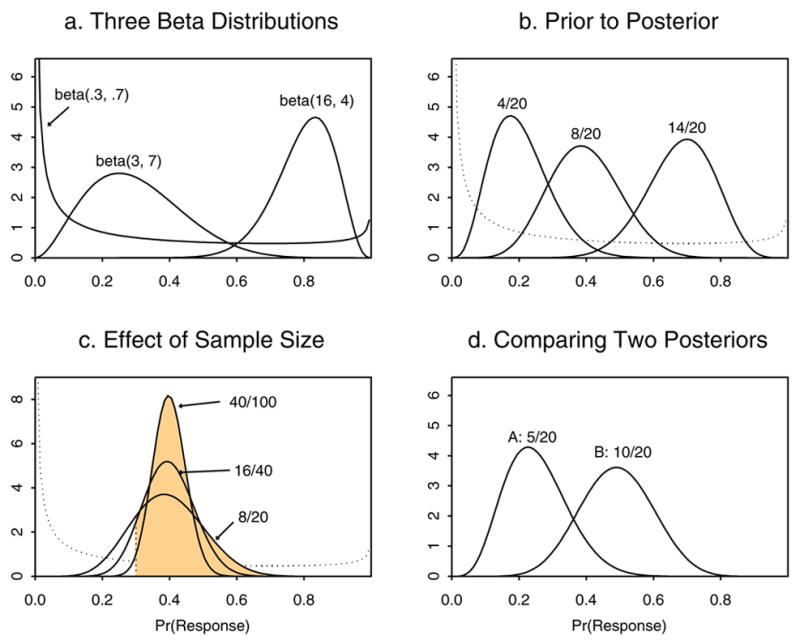
Illustrations of Bayesian priors and posteriors using beta distributions.

4. Bayesian Adaptive Randomization

There is a large literature on adaptive randomization methods, both frequentist^21–23 and Bayesian.^24,25 Actual application of these methods to conduct clinical trials has been quite limited, however.^26–28 In this paper, we will focus on some BAR methods that we have found to work well in practice. The basic idea underlying BAR was first proposed by Thompson²⁹, who showed how to compute p_{A < B}(data) numerically from data of the form described above using paper-and-pencil methods. While p_{A < B}(data) is an intuitively appealing quantity to use as a BAR criterion, if one randomizes patients adaptively to B with probability p_{A < B}(data) and to A with probability p_{A > B}(data) = 1− p_{A < B}(data), this leads to a procedure with some very undesirable properties. The problem is that p_{A < B}(data) is so variable that it produces a substantial risk of unbalancing the samples in favor of the inferior treatment, the opposite of what BAR aims to do, and it also gives a very low probability of selecting a superior treatment (power). These problems may be fixed by a simple modification that stabilizes the randomization probabilities, specifically, randomizing the patient to B with probability

$${\text{r}}_{\text{B}}(\text{data})=\frac{{\{{\text{p}}_{\text{A}<\text{B}}\text{(data)}\}}^{\text{c}}}{{\{{\text{p}}_{\text{A}<\text{B}}\text{(data)}\}}^{\text{c}}+{\{{\text{p}}_{\text{A}>\text{B}}\text{(data)}\}}^{\text{c}}}$$

and to A with probability r_A(data) = 1 − r_B(data), where c is a positive tuning parameter. We call this BAR(c). The value c = 0 gives conventional randomization, and c = 1 gives r_B(data) = p_{A < B}(data), so a value of c between 0 and 1 should be used in practice. While we have found that c = 1/2 works well in many applications, a relatively new BAR procedure with very desirable properties is obtained by setting c = n/2N, where n is the current sample size when a new patient is enrolled and N is the trial's maximum sample size. This method, BAR(n/2N), begins with c = 0 at the start of the trial and ends up with c = 1/2. BAR(n/2N) has the advantages that it preserves power while avoiding the variability of BAR(1).

As a first illustration, we describe a hypothetical trial to compare the response probabilities θ_A and θ_B of treatments A and B. Up to N = 200 patients are randomized, with the trial stopped early and A selected as better than B if p_{B < A}(data) > .99, or B selected if p_{A < B}(data) > .99. Table 1 summarizes computer simulation results for the trial conducted using CR = conventional randomization, BAR(1) and BAR(n/2N). For the BAR methods, beta(.5,.5) priors were assumed for θ_A and θ_B. Binary responses were simulated assuming that θ_A = .25, with θ_B = .30, .35, .40 or .45. Each case was simulated 10,000 times. Table 1 shows that the sample size imbalance in favor of the superior treatment, N_B − N_A, has much larger mean values for BAR(1) than for BAR(n/2N). Thus, it appears that BAR(1) is greatly superior to BAR(n/2N). Looking at the mean values alone is very misleading, however. The 2.5^th and 97.5 ^th percentiles of the distributions of N_B − N_A show that BAR(1) is much more variable than BAR(n/2N). This results in a much higher risk with BAR(1) that the sample imbalance will be in the wrong direction, in favor of the inferior treatment. This is shown by the values of Pr(N_A > N_B + 20), the probability that the number of patients randomized to the inferior arm will be more than 20 larger than the number receiving the superior treatment. Moreover, while the correct selection probabilities (power figures) and mean overall sample sizes for BAR(n/2N) are nearly identical to those obtained with CR, BAR(1) has a much lower power and a much larger overall sample size. In summary, we recommend using BAR(n/2N) because it is likely to provide a substantial sample size imbalance in favor of the superior treatment, has a negligible risk of unbalancing the samples in the wrong direction, and maintains virtually the same power and mean overall sample size as CR.

Table 1.

Operating characteristics of a trial with maximum sample size N = 200 patients and early stopping with selection of the superior treatment if either Pr(θ_A < θ_B | data) > .99 or < .01, using Bayesian adaptive randomization, BAR, with tuning parameter c = 1 or c = n/2N, or conventional randomization, CR. N_A and N_B denote the numbers of patients randomized to A and B. In all cases, θ_A = .25. Each case was simulated 10,000 times.

θB	Randomization Method	Mean (2.5th, 97.5th) of NB − NA	Pr(NA>NB+20)	% Select B (A)	Mean Sample SIze
.30	CR	0 (−26, 26)	.050	25 (6.5)	154
	BAR(1)	39 (−178, 188)	.258	19 (5.0)	173
	BAR(n/2N)	13 (−44, 68)	.090	24 (6.7)	154
.35	CR	0 (−24, 24)	.045	45 (3.5)	136
	BAR(1)	66 (−166, 188)	.140	30 (2.8)	164
	BAR(n/2N)	20 (−24, 72)	.030	44 (3.8)	135
.40	CR	0 (−23, 23)	.034	68 (2.5)	108
	BAR(1)	78 (−128, 186)	.078	44 (1.8)	146
	BAR(n/2N)	20 (−8, 74)	.005	65 (2.5)	112
.45	CR	0 (−20, 20)	.024	85 (1.4)	84
	BAR(1)	81 (−62, 186)	.048	58 (0.9)	130
	BAR(n/2N)	15, (−8, 70)	.001	84 (1.4)	86

Figures 2 and 3 illustrate how a single trial might proceed in a case where B is superior to A. Figure 2 shows the raw data, the posteriors of θ_A and θ_B, and p_{A < B}(data) after n = 50, 100, 150 and 200 patients have been enrolled. In this example, the sample size imbalance in favor of B becomes substantial by n = 150, where the response rates are 41% for B versus 25% for A, and N_B − N_A = 87 − 63 = 24. By n = 200, the imbalance becomes N_B − N_A = 126 − 74 = 52, with 63% of the 200 patients randomized to B. Figure 3 shows the sample path of the adaptive randomization probability values r_B(data) over the course of the trial, as well as the point at n = 145 patients where the trial would have been stopped early with B declared superior. Thus, the trial would have ended with empirical response rates 26% for A and 43% for B, and with N_B − N_A = 83 − 62 = 21 more patients randomized to B.

Fig. 2.

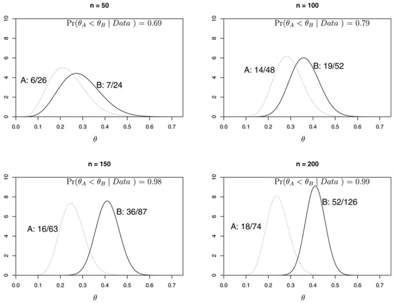
Illustration of the priors and posteriors of response probabilities θ_A and θ_B after 50, 100, 150 and 200 patients for a hypothetical trial conducted using BAR(n/2N).

Fig. 3.

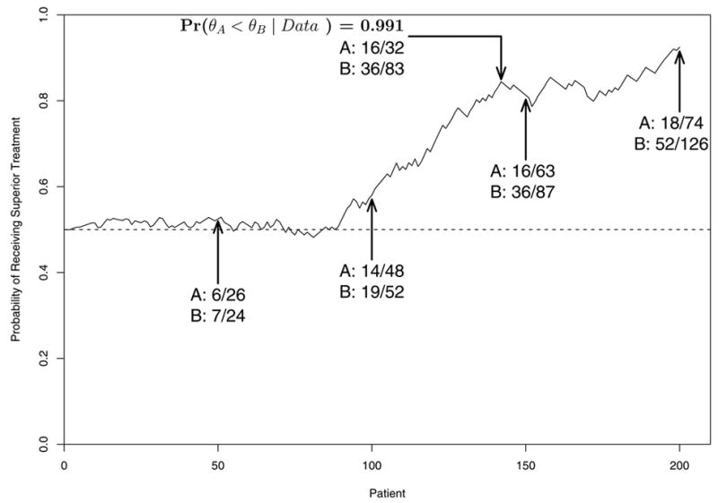
Illustration of the adaptive randomization probabilities over the course of a hypothetical trial conducted using BAR(n/2N).

5. An Adaptively Randomized Sarcoma Trial

BAR was used to conduct a recently completed multi-center trial of gemcitabine + docetaxel (G+D) versus gemcitabine alone (G) for patients with advanced/metastatic unresectable soft tissue sarcoma.^28,30 Initially, a single-arm trial of G+D was planned with the aim to compare the results to historical data on G to assess the G+D-versus-G (docetaxel) effect. When we proposed a randomized trial of G+D versus G to avoid between-trial effects, this created ethical concerns among some investigators who believed G+D likely to be superior. As a compromise, we then proposed a design using BAR, and after resolution of various technical details the design was accepted and implemented.

Each patient received up to four 6-week stages of chemotherapy. In each stage, the patient's outcome was categorized as R = response, defined as a 30% or greater decrease in tumor mass compared to baseline, S = stable disease, or treatment failure F = progressive disease or death. At each of the first three evaluations, the patient's treatment was continued if S was observed, and terminated if either R or F occurred. Overall treatment success could occur with a response at stages 1, 2, 3 or 4 as (R), (S,R), (S,S,R) or (S,S,S,R), and similarly the four cases for overall treatment failure were (F), (S,F), (S,S,F) or (S,S,S,F). Two covariates were considered important: whether the patient had received prior pelvic radiation (PPR), and whether the patient's disease was leiomyosarcoma (LMS) or another type of sarcoma. This produced four subgroups: (LMS, PPR), (Not LMS, PPR), (LMS, No PPR), (Not LMS, No PPR). The trial thus included the complications that each patient's overall outcome could occur in 1, 2, 3 or 4 stages, the outcome in each stage was trinary, {R,S,F}, patients were heterogeneous, and it was thought that the treatment effects might differ across subgroups. To account for all of these factors, we formulated a Bayesian generalized logistic regression model for the probabilities of overall treatment success, π_R, and overall failure, π_F, including effects of treatment, stage, covariates, and treatment-covariate interactions.²⁸ In particular, the model borrows strength across subgroups, in contrast with the simpler but much less reliable approach of conducting four separate trials, one within each subgroup.

To reflect the investigators' subjective opinion that decreasing π_F was 30% more important than increasing π_R, a form of BAR(1/2) was used based on the weighted average θ = π_R + 1.3(1 − π_F). Denoting subgroup by Z, and writing the weighted average as θ_G(Z) for a patient in subgroup Z treated with G and θ_G+D(Z) for a patient in subgroup Z treated with G+D to reflect the patient's subgroup and assigned treatment, the BAR criterion probability was p_G+D(Z, data) = Pr{θ_G(Z) < θ_G+D(Z) | data}, generalizing the formula p_{A < B}(data) given in section 4. A patient in subgroup Z was randomized to G+D with probability

$${\text{r}}_{\text{G}+\text{D}}(\text{data})=\frac{{\left\{{\text{p}}_{\text{G}+\text{D}}(\text{Z},\text{\hspace{0.17em}data})\right\}}^{1/2}}{{\left\{{\text{p}}_{\text{G}+\text{D}}\text{(Z},\text{ data})\right\}}^{1/2}+{\{1-{\text{p}}_{\text{G}+\text{D}}\text{(Z},\text{ data})\}}^{1/2}}$$

and to G with probability 1 − r_G+D(data). In particular, the adaptive randomization probabilities were allowed to differ among the four subgroups determined by PPR and LMS. The trial was designed to accrue up to 120 patients, with accrual suspended in subgroup Z if p_G+D(Z, data) ≥ .99 or ≤ .01, allowing the possibility of re-starting accrual in that subgroup if p_G+D(Z, data) later moved back into the interval (.01, .99) based on subsequent data. Numerical results of an extensive computer simulation study²⁸ showed that this design reliably accounts for treatment-covariate interactions, is likely to provide desirable imbalances in favor of the superior treatment within each subgroup, and has high correct selection probabilities under a wide range of different possible cases.

The trial's sample sizes and posterior probabilities for treatment comparison are summarized in Table 2. After the trial was completed, final data review showed that the covariates of some patients had been entered into the website database incorrectly. Although the covariate data entry errors did not have a severe adverse effect on the trial's outcome, the BAR method did not function as well as it would have had all covariates been entered correctly. While G+D showed superiority over G to some degree in all subgroups, the advantage with G+D was largest in patients with PPR. Avoiding this sort of data entry error is particularly important in trials, such as those using BAR, conducted using adaptive decision rules based on interim data. A lesson here is that an extra level of quality control, to rapidly validate the accuracy of newly entered data, is needed when implementing adaptive methods.

Table 2.

Sample sizes by subgroups for the adaptively randomized trial of gemcitabine + docetaxel (G+D) versus gemcitabine (G). “Website" refers to the data that included some incorrect covariates, while “Actual" refers to the corrected data.

Subgroup	Data Source	Number of Patients		Pr{θG(Z) < θG+D(Z) | data}
LMS, PPR		G+D	G
Yes, No	Website	24	12	.96
	Actual	19	6	.52
Yes, Yes	Website	10	6	.90
	Actual	10	3	.91
No, No	Website	29	24	.71
	Actual	36	32	.79
No, Yes	Website	10	7	.66
	Actual	8	8	.97
Total		73	49

6. Discussion and Practicalities

Since BAR uses the current data to compute the randomization probability for each patient at the time of enrollment, modern computing facilities and efficient data capture are required for practical implementation. In general three computer programs are required: a database, a program to carry out the statistical computations underlying the adaptive decision rules, and a user interface. The interface provides a user-friendly environment for enrolling patients and entering data, and communicates with the database and the program that performs the statistical computations. Essentially, the interface acts as an interactive patient log that asks for specific data and tells the user what actions to take. In multi-institution trials, the interface is best implemented via a secure internet website. Developing this structure requires close interactions among physicians, research nurses, statisticians and programmers.

Before conducting a trial using BAR, or more generally any outcome-adaptive statistical design, it is essential to first establish the design's average properties by simulating the trial many times on the computer under each of set of meaningful possible cases. It also is very useful to examine the design's patient-by-patient behavior in a few simulated individual trials. Based on such preliminary simulations, one may modify the design's parameters, and repeat this procedure until a design with good properties is obtained.

A number of scientific issues arise with the use of adaptive randomization. Since the variability associated with a statistical estimator of a comparative treatment effect θ_A − θ_B is smallest when the sample is allocated equally to A and B, the goal of BAR is at odds with the goal of optimizing precision. Thus, a less precise estimator is a trade-off for the greater ethical desirability of BAR. In this regard, it must be kept in mind that a randomized trial never conducted due to ethical concerns provides no data at all and hence no estimator of θ_A − θ_B. Another concern is that the characteristics of patients enrolled in the trial may change systematically over time, a phenomenon known as “drift," and this may cause an adaptive randomization procedure to function poorly. While the use of a model accounting for covariates, such as that used in the sarcoma trial, reduces the likelihood of this problem, drift due to latent variable effects is an important concern. Methods to deal with drift have been proposed,²² and as new adaptive randomization methods are developed and put into practice it will be important that they correct for the possibility of drift.

A controversial issue in Bayesian clinical trial design is specification of a prior. In Bayesian data analysis it is routine to use several priors, each reflecting a different degree of prior optimism or uncertainty, to assess the sensitivity of posterior inferences to the prior. While this can and should be done when developing a Bayesian clinical trial design, only one prior may be used for trial conduct. Consequently, it is essential this the prior not contain information that may be considered inappropriate. However, the final data may be analyzed using an array of priors, as described above, and not only the prior used for trial conduct.

Our aim has been to convince some readers that BAR may be a desirable alternative to conventional randomization. Certainly, this methodology is complicated and requires a much greater effort in both design and trial conduct. It does, however, utilize the accruing data in a “learn-as-you-go" fashion that arguably makes more sense than ignoring the trial's data until it is completed. Technicalities aside, if a trial is conducted using adaptive randomization, the physician may inform the patient in the following somewhat more reasonable way:

“Mm. Fornier, I have two possible treatments for your cancer, A and B, but I do not know which is better. So I would like to enroll you in a clinical trial aimed at comparing these treatments to each other. If you agree to enter the trial, your treatment will be chosen randomly by a computer, based on the data that we have so far on how well these two treatments have done with previous patients in the trial.

References

- 1.Fisher RA. The Design of Experiments. Edinburgh; Oliver and Boyd: 1935. [Google Scholar]
- 2.Zelen M. The randomization and stratification of patients to clinical trials. J Chronic Diseases. 1974;27:365–375. doi: 10.1016/0021-9681(74)90015-0. [DOI] [PubMed] [Google Scholar]
- 3.Hill AB. Medical ethics and controlled trials. British Medical J. 1963;1:1043–1049. doi: 10.1136/bmj.1.5337.1043. [DOI] [PMC free article] [PubMed] [Google Scholar]
- 4.Freedman B. Equipoise and the ethics of clinical research. New England J Medicine. 1987;317:141–145. doi: 10.1056/NEJM198707163170304. [DOI] [PubMed] [Google Scholar]
- 5.Royall RM. Ethics and statistics in randomized clinical trials (with discussion) Statistical Science. 1991;6:52–88. doi: 10.1214/ss/1177011934. [DOI] [PubMed] [Google Scholar]
- 6.Emanuel EJ, Patterson WB. Ethics of randomized clinical trials. J Clinical Oncology. 1998;48:6–29. doi: 10.1200/JCO.1998.16.1.365. [DOI] [PubMed] [Google Scholar]
- 7.Ashcroft R. Equipoise, knowledge and ethics in clinical research and practice. Bioethics. 1999;13:314–326. doi: 10.1111/1467-8519.00160. [DOI] [PubMed] [Google Scholar]
- 8.Cox DR. Regression models and life tables (with discussion) J Royal Statistical Soc, B. 1972;34:187–220. [Google Scholar]
- 9.Estey EH, Thall PF. New designs for phase 2 clinical trials. Blood. 2003;102:442–448. doi: 10.1182/blood-2002-09-2937. [DOI] [PubMed] [Google Scholar]
- 10.Gail MH, Wieand S, Piantadosi S. Biased estimates of treatment effect in randomized experiments with nonlinear regressions and omitted covariates. Biometrika. 1984;71:431–444. [Google Scholar]
- 11.Localio AR, Berlin JA, Ten Have TR, Kimmel SE. Adjustments for center in multicenter studies: an overview. Ann Internal Medicine. 2001;135:112–123. doi: 10.7326/0003-4819-135-2-200107170-00012. [DOI] [PubMed] [Google Scholar]
- 12.Pocock SJ. Clinical Trials: A Practical Approach. New York: Wiley; 1984. [Google Scholar]
- 13.Piantadosi S. Clinical Trials. New York: Wiley; 1997. [Google Scholar]
- 14.Rosenberger WF, Lachin JM. Randomization in Clinical Trials: Theory and Practice. New York: Wiley; 2002. [Google Scholar]
- 15.Gelman A, Carlin JB, Stern HSA, Rubin DB. Bayesian Data Analysis. 2. Boca Raton: Chapman and Hall/CRC; 2004. [Google Scholar]
- 16.Smith AFM, Gelfand AE. Bayesian statistics without tears: A sampling resampling perspective. American Statistician. 1992;46:84–88. [Google Scholar]
- 17.Spiegelhalter D, Thomas A, Best N, Gilks W. BUGS: Bayesian Inference Using Gibbs Sampling, Version 0.50. MRC Biostatistics Unit; Cambridge, UK: 1995. [Google Scholar]
- 18.Berry DA, Stangl DK, editors. Bayesian Biostatistics. New York: Marcell Dekker; 1996. [Google Scholar]
- 19.Berry DA. A case for Bayesianism in clinical trials (with discussion) Stat in Medicine. 1993;12:1377–1404. doi: 10.1002/sim.4780121504. [DOI] [PubMed] [Google Scholar]
- 20.Spiegelhalter DJ, David J, Abrams KR, Myles JP. Bayesian Approaches to Clinical Trials and Health-Care Evaluation. New York: John Wiley & Sons; 2004. [Google Scholar]
- 21.Zelen M. A new design for randomized clinical trials. New England J Medicine. 1979;300:1242–1246. doi: 10.1056/NEJM197905313002203. [DOI] [PubMed] [Google Scholar]
- 22.Karrison TG, Huo D, Chappell R. A group sequential, response-adaptive design for randomized clinical trials. Controlled Clinical Trials. 2003;24:506–522. doi: 10.1016/s0197-2456(03)00092-8. [DOI] [PubMed] [Google Scholar]
- 23.Hu F, Rosenberger WF. Response Adaptive Randomization. Hoboken: Wiley; 2006. [Google Scholar]
- 24.Berry DA, Eick SG. Adaptive assignment versus balanced randomization in clinical trials: a decision analysis. Stat in Medicine. 1995;14:231–246. doi: 10.1002/sim.4780140302. [DOI] [PubMed] [Google Scholar]
- 25.Cheung YK, Inoue LYT, Wathen JK, Thall PF. Continuous Bayesian adaptive randomization based on event times with covariates. Stat in Medicine. 2006;25:55–70. doi: 10.1002/sim.2247. [DOI] [PubMed] [Google Scholar]
- 26.Bartlett RH, Roloff DW, Cornell RG, Andrews AF, Dillon PW, Zwischenberger JB. Extra-corporeal circulation in neonatal respiratory failure: A prospective randomized study. Pediatrics. 1985;76:476–487. [PubMed] [Google Scholar]
- 27.Thall PF, Inoue LYT, Martin T. Adaptive decision making in a lymphocyte infusion trial. Biometrics. 2002;58:560–568. doi: 10.1111/j.0006-341x.2002.00560.x. [DOI] [PubMed] [Google Scholar]
- 28.Thall PF, Wathen JK. Covariate-adjusted adaptive randomization in a sarcoma trial with multi-stage treatments. Stat in Medicine. 2005;24:1947–1964. doi: 10.1002/sim.2077. [DOI] [PubMed] [Google Scholar]
- 29.Thompson WR. On the likelihood that one unknown probability exceeds another in view of the evidence of two samples. Biometrika. 1933;25:285–294. [Google Scholar]
- 30.Maki RG, Hensley ML, Wathen JK, Patel SR, Priebat DA, Okuno S, Reinke D, Thall PF, Benjamin RS, Baker LH. A SARC multicenter phase III study of gemcitabine vs. gemcitabine and docetaxel in patients with metastatic soft tissue sarcomas. J Clinical Oncology. 2006;24(18S):9514. [Google Scholar]