Frequency-Dependent Selection in a Periodic Environment

Abstract

We examine the action of natural selection in a periodically changing environment where two competing strains are specialists respectively for each environmental state. When the relative fitness of the strains is subject to a very general class of frequency-dependent selection, we show that coexistence rather than extinction is the likely outcome. This coexistence may be a stable periodic equilibrium, stable limit cycles of varying lengths, or be deterministically chaotic. Our model is applicable to the population dynamics commonly found in many types of viruses.

1 Introduction

The most commonly used theoretical framework to study the dynamics of viral populations is the quasispecies model [1–5], which predicts an equilibrium state in which a single dominant sequence—the master sequence—is surrounded by a stable cloud of closely related mutant sequences. However, the basic quasispecies model neglects a number of effects known to be highly relevant for virus replication and survival. First, the quasispecies model is usually studied for constant environmental conditions (but see [6–8]), even though viruses frequently experience changing environments. In particular, arboviruses, which include examples such as West Nile virus and dengue-fever virus, regularly alternate host species between arthropods and vertebrates, and experimental efforts have demonstrated that arboviruses readily adapt to alternating conditions [9–15]. Second, the quasispecies model assumes low virus density (as measured by the number of infecting virus particles per cell, also multiplicity of infection or MOI), but high virus density is common in many systems and can lead to drastically altered competition dynamics [16–26].

One common observation at high MOI is the presence of frequency-dependent selection [19–21]. While the frequency dependence of a strain’s fitness may take many functional forms, a common type is where the strain competes best when it is rare relative to its competitor. This form of “fittest when rare” frequency dependence naturally arises under biological conditions of parasitism or through the evolution of cheating strategies. Viral deletion mutants known as defective interfering particles (DIPs) are viral parasites commonly found under conditions of high MOI [22–25]. No longer capable of independent reproduction themselves, DIPs rely on co-opting wild type viral products in an infected cell, and have a selective advantage over the wild type due to the faster replication of their smaller genome [27,28]. Game theoretic models have been applied to conditions of viral coinfection, where selfish behavior similar to that in the prisoner’s dilemma evolved [26,29,21]. Such selfish strategies naturally work best rare, suffering when common from a lack of others to exploit.

Motivated by these common features of viral systems, we develop a theoretical model to study competition between two strains in a periodic environment. Each strain is relatively well adapted to one environment, but poorly adapted to the other. In this context, we model the general effects of frequency-dependent selection under the simplifying assumption that the strains compete best when rare. For a wide range of competitive conditions, our model predicts coexistence of both strains. This coexistence may be as simple as a periodic alternation of population sizes synchronized with environmental changes, or as complex as fully chaotic population dynamics.

2 Model

The competition between two strains, A and B, occurs in a time dependent environment which oscillates between two distinct states. We assume the limit of large population size and describe the current state of the population by x, the population fraction of strain A. To characterize the fitness of each strain, we normalize the fitness of the superior strain to be 1, and describe the relative fitness of the inferior strain by a frequency-dependent fitness function w(x). During environmental state 1, therefore, strain A is superior and has a constant normalized fitness w_A = 1, while strain B is inferior with frequency-dependent fitness 0 < w_B(x) < 1. Consistent with our assumption that strain B competes best when rare, we take w_B(x) to be a monotonically increasing function. For definiteness, we denote relative fitness of strain B when very common as b₀ = w_B(0) and the fitness of strain B when very rare as b₁ = w_B(1), where b₀ ≤ b₁ by assumption. If the population starts in environment 1 with a population fraction of strain A given by x, it will have a fraction f₁(x) at the end given by

$$f_1(x)=\frac{x}{x+(1-x)w_B(x)}.$$ (1)

In environmental state 2, the roles of the strains reverse. Strain B is superior with normalized fitness w_B = 1 while strain A is inferior with frequency-dependent fitness w_A(x). This means that w_A(x) is a monotonically decreasing function, and we denote the values a₁ = w_A(0) and a₀ = w_A(1) where a₀ ≤ a₁. Let f₂(x) give the population fraction at the close of environment 2, given that it began environment 2 with population x. Then we have

$$f_2(x)=\frac{x{w}_A(x)}{(1-x)+x{w}_A(x)}.$$ (2)

We will make the biologically reasonable assumption that both fitness functions w_A(x) and w_B(x) are continuous. Under these assumptions, there are three qualitatively different relationships possible between the relative fitness functions w_A and w_B: One or the other can be strictly larger for all values of x, or the fitness functions can cross at some intermediate value of x. These three cases are show schematically in Fig. 1. Note that the applicable case can be determined solely by considering the relative magnitudes of the four constants a₀, a₁, b₀, and b₁.

Fig. 1.

Three cases of qualitatively different relationships between the frequency dependence of fitness functions w_A(x) and w_B(x). Case I, left: Strain B is strictly superior. Case II, middle: Neither strain is strictly superior. Case II, right: Strain A is strictly superior.

3 Results

3.1 Existence of Equilibria

We prove that the cases I and III from Fig. 1 allow for no stable coexistence between strains, and extinction occurs as the population fraction converges to x = 0 or x = 1 respectively. Conversely, in case II there is always an equilibrium value of x ∈ (0, 1) where both strains coexist. The stability of this equilibrium, however, is more complicated and will be addressed later. If we assume the population begins a period at x in environment 1, it will end the period with population g(x) given by

$$g(x)=f_2[f_1(x)]=\frac{x{w}_A(y)}{w_B(x)+x[w_A(y)-w_B(x)]},$$ (3)

where y = f₁(x). An equilibrium in the periodic environment corresponds to a solution of the equation g(x) = x. We shall henceforth refer to such a solution as an equilibrium, even though the population is actually alternating between two different values, x and f₁(x), as the environmental state changes. We shall refer to a periodic equilibrium as a situation where, for example, g(x) alternates between two different values (and the population alternates between four different values before repeating the pattern). An equilibrium point x will be a locally stable or attracting equilibrium if |g′(x)| < 1 and locally unstable or repelling if |g′(x)| > 1. Assuming the equilibrium value does not correspond to extinction, x ≠ 0, 1, we find that there can be a solution to g(x) = x if and only if

$$w_A(y)=w_B(x).$$ (4)

In the cases I or III, the ranges of w_A(x) and w_B(x) are disjoint, and hence there can be no solution to Eq (4). Therefore the only equilibrium solutions in these cases are x = 0 or 1, and testing the derivative g′(x) at these values confirms that x = 0 is attracting while x = 1 is repelling in case I, and vice versa for case III. Qualitatively, strain B wins the competition in case I and strain A wins in case III. Observe that this results corresponds to the strain with the strictly larger relative fitness function in Fig. 1 going to fixation in the population.

To see that there must be an equilibrium in case II, consider the function h(x) = w_A[f₁(x)] − w_B(x). This function is continuous, with h(0) = a₁ − b₀ > 0 and h(1) = a₀ − b₁ < 0. Thus by the Intermediate Value Theorem, there exists an x_e ∈ (0, 1) where h(x_e) = 0. By construction, this x_e satisfies Eq. (4) and hence x_e is an equilibrium corresponding to coexistence of both strains. The values x = 0 and x = 1, corresponding to extinction of either strain, are repelling equilibria. This result can be seen by evaluating g′(x), where we find g′(0) = b₁/a₀ > 1 and g′(1) = a₁/b₀ > 1. Thus in case II, neither strain will suffer extinction in an infinite population. However, the equilibrium at x_e need not be stable in this case. For example, there could be an attracting periodic cycle or other more complex behavior. In the case of many simple fitness functions we can rule out these complex behaviors, as we show in the next section.

The stable coexistence of strains in case II is more remarkable given how likely it is to occur. While the precise relative probabilities of the three cases will depend on the specific biological system in question, we can qualitatively address this issue by assuming the endpoints of the fitness functions a₀, a₁, b₀, and b₁ are chosen uniformly at random in [0, 1], consistent with the requirement that a₀ ≤ a₁ and b₀ ≤ b₁. Under these assumptions, basic probabilistic considerations show that we expect case II to occur 2/3 of the time, while cases I and III occur with probability 1/6 each.

3.2 Stable Coexistence in the Linear Case

Consider the special case when the functions w_A(x) and w_B(x) are linear functions,

$$w_A(x)=a_1-(a_1-a_0)x,$$ (5)

$$w_B(x)=b_0+(b_1-b_0)x.$$ (6)

In this case, we shall prove that there is a unique stable equilibrium when the fitness functions meet the conditions of case II. To see that the equilibrium is unique, consider the function w_A(y) that appears in Eq (4). Computing its derivative, we find that that it is a decreasing function,

$$\frac{d{w}_A(y)}{dx}=\frac{d{w}_A(y)}{dy}\frac{d{f}_1(x)}{dx}<0.$$ (7)

While dw_A(y)/dy is always negative since w_A(y) is a decreasing function, the result of Eq. (7) only holds because df₁(x)/dx is strictly positive in the linear case. Therefore, when we solve the equilibrium equation w_A(y) = w_B(x), we are seeking the intersections between a strictly increasing function, w_B(x), and a strictly decreasing function, w_A(y). Assuming we are in case II where an equilibrium exists for x ∈ (0, 1), the equilibrium must be unique.

Moreover, this equilibrium is stable. Observe that for any fitness function, including nonlinear ones, f₂(x) is increasing since df₂(x)/dx > 0. In the linear case, direct calculation shows that df₁(x)/dx > 0 and therefore g(x) is also an increasing function,

$$\frac{dg}{dx}=f_2^{\prime }[f_1(x)]\frac{d{f}_1(x)}{dx}>0.$$ (8)

It is impossible for the increasing function g(x) to have any oscillatory behavior. Since the values x = 0 and x = 1 are known to be repelling fixed points for case II, the remaining equilibrium must be a stable fixed point.

3.3 A Stability Condition

Our above proof that a unique and stable equilibrium exists in the case of linear fitness functions can be generalized. The key condition is proving that g(x) is increasing. While df₂(x)/dx > 0 holds for all fitness functions, f₁(x) may not be increasing. In general, we have

$$\frac{d{f}_1(x)}{dx}=\frac{w_B(x)-x(1-x)w_B^{\prime }(x)}{{[x+(1-x)w_B(x)]}^2}.$$ (9)

Although w′_B(x) > 0 by assumption, $f_1^{\prime }(x)$ could be negative if the fitness function w_B(x) changes very rapidly as a function of the population fraction x. A sufficient but not necessary condition for stable coexistence is therefore

$$w_B(x)\ge x(1-x)w_B^{\prime }(x)\hspace{0.17em}\forall x\in [0,1].$$ (10)

We now give an example where rapid change in the frequency-dependent fitness leads to more complex population dynamics.

3.4 Chaotic Dynamics in the General Case

In general, the population dynamics of our system can be chaotic. As an example, consider the case that strain A has no frequency dependence, that is, w_A(x) is constant. We take w_B(x) to smoothly change from a straight line to a step function as the parameter a increases. The fitness functions for this example are shown in Fig. 2, including w_B(x) for varying values of the parameter a. The specific functions used in this example are

Fig. 2.

Sample fitness function w_A(x) (solid line) and functions w_B(x) (broken lines) given in Eq. (11). Parameter values for w_B(x) are a = 10⁻², 1, 10², 10⁴.

$$w_A(x)=\frac{2}{5},\hspace{0.17em}\hspace{0.17em}\hspace{0.17em}{w}_B(x)=\frac{1}{2}+\frac{4}{5\pi }\text{ArcTan}\left[a\left(x-\frac{1}{2}\right)\right].$$ (11)

An important result in the theory of one dimensional iterated maps is Sarkovskii’s Theorem [30], sometimes referred to as “Period Three Implies Chaos” [31]. This theorem states that whenever a continuous map has a point of period 3 it has points of all period lengths, a common property of chaotic systems. Points of period 3 appear in our example once the parameter a ≳ 10² (see also Fig. 3). For instance, when a = 10³, we are in the domain of an attracting 8-cycle. In this case, there are still points of period 3 (and hence all periods), but these other periodic points are unstable. One of these unstable period 3 cycles is shown in Fig. 4 converging quickly to the stable 8-cycle due to finite precision effects. Several other population trajectories are shown in Fig. 4, illustrating the population dynamics for different parameter values a.

Fig. 3.

Illustration of a 3-cycle on the plot of g(x), using the fitness functions in Eq. (11) and the parameter value a = 10³. The existence of a 3-cycle often indicates the presence of chaos in a system.

Fig. 4.

Population fraction of strain A, as a function of the number of environmental periods. Left to Right: The unstable equilibrium is attracted to the stable 2-cycle (a = 10^1.5); the orbit of x = 1/2 shows unpredictable behavior (a = 10²); an unstable 3 cycle is attracted to the stable 8-cycle (a = 10³).

In Fig. 5, we display the orbits of representative initial points after a large number of iterations (see Appendix for technical details). As the parameter a increases, the attracting equilibrium of the system is no longer a fixed point, but instead becomes a periodic equilibrium. The bifurcations that occur in Fig. 5 with increasing a are one of the classic hallmarks of a chaotic system [32]. For small values of a ≲1, the crossing condition of case II is not met, x = 0 is the stable equilibrium, and strain A goes extinct. For 1 ≲a ≲10, a stable equilibrium allows for coexistence of both strains, with an increasing equilibrium fraction of strain A. For 10 ≲a ≲100, the previous equilibrium is no longer stable, and undergoes a period doubling bifurcation to produce a stable equilibrium of period 2. As a increases beyond this point, the long term behavior of the system becomes increasely complex, although there are occasional windows of relatively short stable periods. In spite of the chaotic dynamics in this case, we can still see from Fig. 5 that the two strains will coexist indefinitely as long as the crossing condition is met, with the population fraction in this case varying within the range x ≈ [0.3, 0.8].

Fig. 5.

Population fraction in steady state, plotted as a function of the parameter a in Eq. (11). We plot the population fraction x for many periods, after allowing a long time for initial equilibration (periods shown are 1000–2000). From left to right, the system shows extinction of one strain, stable coexistence, periodic behavior, and finally chaos. Initial conditions are chosen so that all attracting orbits will be found (see Appendix).

Why do the orbits become increasingly complex as one of the fitness functions becomes more step-like? In the previous subsection, we have given the mathematical reason, which is that Eq. (10) is violated. The intuitive explanation is the following. Assume w_B(x) is close to a step function, with the location of the step given by x*, and w_A(x) is a constant that crosses w_B(x) at x*. Then, for x < x*, strain A is substantially superior to strain B, and for most x < x*, the frequency of strain A after one period, g(x), will be larger than x*. Likewise, for x > x*, strain A is substantially inferior to strain B, and therefore for most x > x*, we will have g(x) < x*. Thus, the step-like fitness function causes x to overshoot its equilibrium value coming both from the left and from the right. The more step-like w_B(x), the more dramatic the overshooting, and therefore the more complex the resulting orbit.

3.5 Noisy Fitness Functions

Equations (1) and (2) assume that we can exactly predict the relative growth of strains A and B in the two environmental states. A more realistic assumption is that the relative growth of the two strains is subject to some noise. The noise could be caused by a variety of factors. For example, the durations of the two environmental states might not always be of exactly the same length, or there might be some intrinsic variability in the two environments. We model these fluctuations by multiplying the frequencies of the two strains at the end of environmental period i with a factor e^±γZ_i/2, where Z_i is a standard normal random variate, and γ is a constant measuring the noise intensity. Since the distribution of Z_i is symmetric about zero, and we can arbitrarily renormalize the fitness of either strain to one, the model with noise is equivalent to writing

$$\begin{array}{l}{f}_1(x)=\frac{x}{x+(1-x)w_B(x)e^{\gamma Z_1}},\\ f_2(x)=\frac{x\hspace{0.17em}{w}_A(x)e^{\gamma Z_2}}{(1-x)+x\hspace{0.17em}{w}_A(x)e^{\gamma Z_2}}.\end{array}$$ (12)

In the presence of noise, the concepts of stable fixed points and periodic orbits become meaningless. Nevertheless, we expect the system’s trajectories to remain in the vicinity of the noiseless orbits as long as the noise is small. Indeed, we observe exactly this behavior when we simulate the system with noise. As we increase the noise level, the trajectories become gradually broader (Fig. 6). The fine details of the bifurcation diagram are lost early, at small noise levels, whereas the broad overall structure remains unchanged even for fairly large noise levels (Fig. 6). One important effect of noise is that the onset of apparent chaos, that is, the blurring out of all the periodic behavior in the phase diagram, happens at much lower values of log a. In other words, in realistic systems where noise is present, we don’t require such steep changes in the frequency-dependent fitness relative to the noiseless case to give rise to complete unpredictability in the system’s behavior. Thus, in summary, both rapid changes in fitness as a function of mutant frequency or the presence of noise accelerate the onset of unpredictable dynamics.

Fig. 6.

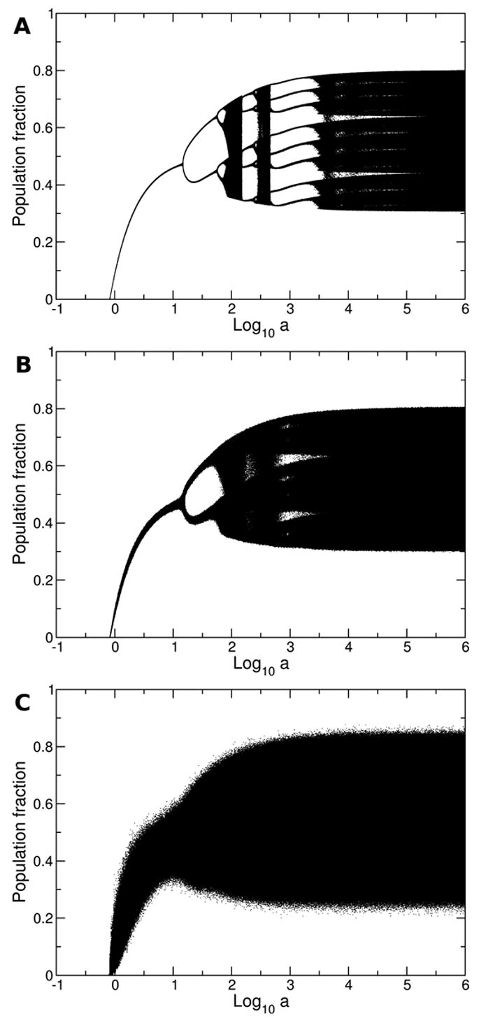
Population fraction in steady state in the presence of noise, plotted as a function of the parameter a in Eq. (11). The noise levels are γ = 0.001 (A), γ = 0.01 (B), and γ = 0.1 (C). All other parameter settings are as in Fig. 5.

4 Discussion

Varying environmental conditions or frequency-dependent selection appear separately in many models of biological populations. Within the field of population dynamics, changing environments have often been associated with promoting stable polymorphisms [33–37], although chaotic dynamics are also possible [38,39]. Frequency-dependent selection is similarly common in biological models, especially where game theoretic strategies are possible [40,41], and can also give rise to chaotic dynamics [42,43].

We present a biologically motivated model of frequency-dependent selection in a periodic environment. Coexistence of both strains is predicted for a wide range of possible fitness assumptions (case II in Fig. 1). The condition for coexistence is that each strain’s relative fitness function is superior to the other’s at some frequency level, and extinction is only possible when one fitness function dominates the other at all frequencies. An experimental consequence of this result is that fitness measurements taken separately in each environmental state for each strain when rare suffice to predict the coexistence or extinction that will result when the strains compete in the periodic environment.

Our model is applicable to viral populations, especially those where defective or complementing viral particles are present. Periodic environmental change is present in commonly studied viral systems, often in the form of alternation between low and high levels of coinfection [44,18]. Models of viral defective particles incorporate frequency dependence [44,45] and show chaotic behavior similar to what we observe [46].

Our results suggests that stable equilibrium, rather than oscillations or chaotic dynamics, is likely for most biological fitness models of the type studied. Only when the relative fitness of the strains changes very rapidly with frequency does the system exhibit periodic behavior or chaos. We offer a simple mathematical test to exclude the possibility of oscillations or chaos in the system for a given model of frequency dependence.

In arboviruses or other viruses that alternate host species, our results suggest that coexistence between the wild type virus and an undetected mutant strain may be quite common. RNA viruses are known for their high mutation rate [47], and consequently many different mutants are produced during viral replication. Consider the evolutionarily favored situation of a mutation that confers an advantage in the current host species, but which may have a negative fitness effect in the alternate host. Our results indicate that such a mutant can persist in the wild-type population as long as the negative fitness effects are frequency dependent and not too severe. As such, what may begin as a single wild type strain may, over time, evolve into two coexisting specialist strains where each adapts well to one host and poorly to the other.

In conclusion, we present a very general model of frequency-dependent selection in a periodic environment. In addition to applications in virology, we expect the generality of our approach will allow this model to be useful broadly within the field of population dynamics and evolutionary ecology.

A Finding all attracting orbits

To understand the dynamics of our system, several results from the mathematics of one dimensional iterated maps are relevant [48,49]. A useful tool in understanding the long term behavior of the system is the Schwarzian derivative of a function g(x), Sg(x):

$$Sg(x)=\frac{g^{‴}(x)}{g^{\prime }(x)}-\frac{3}{2}{\left(\frac{g^{″}(x)}{g^{\prime }(x)}\right)}^2.$$ (A.1)

In the study of iterated maps, functions with strictly negative Schwarzian derivatives, i.e. ∀x Sg(x) < 0, are mathematically well behaved. In particular, when this condition holds there exists a critical point of g(x) [where dg(x)/dx = 0] whose orbit is eventually attracted to any attracting periodic point of the system [32]. Therefore if the Schwarzian derivative is strictly negative, only the critical points of g(x) must be studied to determine the nature of the attracting orbits of the system.

In our chaotic example using the fitness functions given in Eq. (11), once the parameter a exceeds a_c ≈ 10^0.87, we have Sg(x) < 0 for all x. This critical value of a_c can be found either by use of the Schwarzian derivative condition or by solving the stability condition given in Eq. (10). For a larger than the critical value a_c, g(x) has two critical points. These critical points are found numerically and both of their orbits are plotted after a large number of iterations in Fig. 5. Since these critical points converge to an attracting fixed point of the system, we can see all the possible long term behaviors of the system by examining only the orbits of these points.

For values of a less than the cutoff value a_c, there are no critical points of g(x) as dg(x)/dx is strictly positive. This implies that g(x) is an increasing function, and, as in the linear case, this rules out any periodic behavior. For these smaller values of a < a_c, we arbitrarily plot the orbit of x = 1/2 in Fig. 5.

References

- 1.Eigen M, Schuster P. The Hypercycle—A Principle of Natural Self-Organization. Springer-Verlag; Berlin: 1979. [DOI] [PubMed] [Google Scholar]
- 2.Eigen M, McCaskill J, Schuster P. Molecular quasi-species. J Phys Chem. 1988;92:6881–6891. [Google Scholar]
- 3.Domingo E, Biebricher CK, Eigen M, Holland JJ. Quasispecies and RNA Virus Evolution: Principles and Consequences. Landes Bioscience; Georgetown, TX: 2001. [Google Scholar]
- 4.Bull JJ, Meyers LA, Lachmann M. Quasispecies made simple. PLoS Comp Biol. 2005;1:e61. doi: 10.1371/journal.pcbi.0010061. [DOI] [PMC free article] [PubMed] [Google Scholar]
- 5.Wilke CO. Quasispecies theory in the context of population genetics. BMC Evol Biol. 2005;5:44. doi: 10.1186/1471-2148-5-44. [DOI] [PMC free article] [PubMed] [Google Scholar]
- 6.Nilsson M, Snoad N. Error thresholds on dynamic fitness landscapes. Phys Rev Lett. 2000;84:191–194. doi: 10.1103/PhysRevLett.84.191. [DOI] [PubMed] [Google Scholar]
- 7.Wilke CO, Ronnewinkel C, Martinetz T. Dynamic fitness landscapes in molecular evolution. Phys Rep. 2001;349:395–446. [Google Scholar]
- 8.Forster R, Wilke CO. Tradeoff between short-term and long-term adaptation in a changing environment. Phys Rev E. 2005;72:041922. doi: 10.1103/PhysRevE.72.041922. [DOI] [PubMed] [Google Scholar]
- 9.Chen WJ, Wu HR, Chiou SS. E/NS1 modifications of dengue 2 virus after serial passages in mammalian and/or mosquito cells. Intervirology. 2003;46:289–295. doi: 10.1159/000073208. [DOI] [PubMed] [Google Scholar]
- 10.Cooper LA, Scott TW. Differential evolution of eastern equine encephalitis virus populations in response to host cell type. Genetics. 2001;157:1403–1412. doi: 10.1093/genetics/157.4.1403. [DOI] [PMC free article] [PubMed] [Google Scholar]
- 11.Turner PE, Elena SF. Cost of host radiation in an rna virus. Genetics. 2000;156:1465–1470. doi: 10.1093/genetics/156.4.1465. [DOI] [PMC free article] [PubMed] [Google Scholar]
- 12.Novella IS, Clarke DK, Quer J, Duarte EA, Lee CH, Weaver SC, Elena SF, Moya A, Domingo E, Holland JJ. Extreme fitness differences in mammalian and insect hosts after continuous replication of vesicular stomatitis virus in sandfly cells. J Virol. 1995;69:6805–6809. doi: 10.1128/jvi.69.11.6805-6809.1995. [DOI] [PMC free article] [PubMed] [Google Scholar]
- 13.Novella IS, Hershey CL, Escarmis C, Domingo E, Holland J. Lack of evolutionary stasis during alternating replication of an arbovirus in insect and mammalian cells. J Mol Biol. 1999;287:459–465. doi: 10.1006/jmbi.1999.2635. [DOI] [PubMed] [Google Scholar]
- 14.Weaver SC, Brault AC, Kang W, Holland JJ. Genetic and fitness changes accompanying adaptation of an arbovirus to vertebrate and invertebrate cells. J Virol. 1999;73:4316–4326. doi: 10.1128/jvi.73.5.4316-4326.1999. [DOI] [PMC free article] [PubMed] [Google Scholar]
- 15.Zárate S, Novella IS. Vesicular stomatitis virus evolution during alternation between persistent infection in insect cells and acute infection in mammalian cells is dominated by the persistence phase. J Virol. 2004;78:12236–12242. doi: 10.1128/JVI.78.22.12236-12242.2004. [DOI] [PMC free article] [PubMed] [Google Scholar]
- 16.Turner PE, Chao L. Sex and the evolution of intrahost competition in rna virus φ6. Genetics. 1998;150:523–532. doi: 10.1093/genetics/150.2.523. [DOI] [PMC free article] [PubMed] [Google Scholar]
- 17.Novella IS, Reissig DD, Wilke CO. Density-dependent selection in vesicular stomatitis virus. J Virol. 2004;78:5799–5804. doi: 10.1128/JVI.78.11.5799-5804.2004. [DOI] [PMC free article] [PubMed] [Google Scholar]
- 18.Wilke CO, Ressig DD, Novella IS. Replication at periodically changing multiplicity of infection promotes stable coexistence of competing viral populations. Evolution. 2004;58:900–905. doi: 10.1111/j.0014-3820.2004.tb00422.x. [DOI] [PubMed] [Google Scholar]
- 19.Elena SF, Miralles R, Moya A. Frequency-dependent selection in a mammalian RNA virus. Evolution. 1997;51:984–987. doi: 10.1111/j.1558-5646.1997.tb03679.x. [DOI] [PubMed] [Google Scholar]
- 20.Yuste E, Moya A, López-Galíndez C. Frequency-dependent selection in human immunodeficiency virus type 1. J Gen Virol. 2002;83:103–106. doi: 10.1099/0022-1317-83-1-103. [DOI] [PubMed] [Google Scholar]
- 21.Turner PE, Chao L. Escape from prisoner’s dilemma in rna phage φ6. Am Nat. 22003;161:497–505. doi: 10.1086/367880. [DOI] [PubMed] [Google Scholar]
- 22.Huang AS. Defective interfering viruses. Annu Rev Microbiol. 1973;27:101–117. doi: 10.1146/annurev.mi.27.100173.000533. [DOI] [PubMed] [Google Scholar]
- 23.Perrault J. Origin and replication of defective interfering particles. Curr Top Microbiol Immunol. 1981;93:151–207. doi: 10.1007/978-3-642-68123-3_7. [DOI] [PubMed] [Google Scholar]
- 24.Roux L, Simon AE, Holland JJ. Effects of defective interfering viruses on virus replication and pathogenesis in vitro and in vivo. Adv Virus Res. 1991;40:181–211. doi: 10.1016/S0065-3527(08)60279-1. [DOI] [PMC free article] [PubMed] [Google Scholar]
- 25.García-Arriaza J, Manrubia SC, Toja M, Domingo E, Escarmís C. Evolutionary transition toward defective rnas that are infectious by complementation. J Virol. 2004;78:11678–11685. doi: 10.1128/JVI.78.21.11678-11685.2004. [DOI] [PMC free article] [PubMed] [Google Scholar]
- 26.Turner PE, Chao L. Prisoner’s dilemma in an rna virus. Nature. 1999;398:441–443. doi: 10.1038/18913. [DOI] [PubMed] [Google Scholar]
- 27.Mills DR, Peterson RL, Spiegelman S. An extracellular darwinian experiment with a self-duplicating nucleic acid molecule. Proc Natl Acad Sci USA. 1967;58:217–224. doi: 10.1073/pnas.58.1.217. [DOI] [PMC free article] [PubMed] [Google Scholar]
- 28.Sabo DL, Domingo E, Bandle EF, Flavell RA, Weissmann C. A guanosine to adenosine transition in the 3′ terminal extracistronic region of bacteriophage qb rna leading to loss of infectivity. J Mol Biol. 1977;112:235–252. doi: 10.1016/s0022-2836(77)80141-1. [DOI] [PubMed] [Google Scholar]
- 29.Lenski RE, Velicer GJ. Games microbes play. Selection. 2000;1:89–95. [Google Scholar]
- 30.Sarkovskii AN. Coexistence of cycles of a continuous map of a line into itself. Ukrain Mat Z. 1964;16:61–71. [Google Scholar]
- 31.Li TY, Yorke JA. Period three implies chaos. Am Math Monthly. 1975;82:985–992. [Google Scholar]
- 32.Devaney RL. A first course in chaotic dynamical systems. Addison-Wesley; Boston: 1992. [Google Scholar]
- 33.Kirzhner VM, Korol AB, Ronin YI. Cyclical environmental changes as a factor in maintaining genetic polymorphism. J Evol Biol. 1995;8:93–120. doi: 10.1111/j.1558-5646.1996.tb03917.x. [DOI] [PubMed] [Google Scholar]
- 34.Bürger R. Evolution of genetic variability and the advantage of sex and recombination in changing environments. Genetics. 1999;153:1055–1069. doi: 10.1093/genetics/153.2.1055. [DOI] [PMC free article] [PubMed] [Google Scholar]
- 35.Suiter AM, Banziger O, Dean AM. Fitness consequences of a regulatory polymorphism in a seasonal environment. Evolution. 2003;100:12782–12786. doi: 10.1073/pnas.2134994100. [DOI] [PMC free article] [PubMed] [Google Scholar]
- 36.Edwards RJ, Brookfield JFY. Transiently beneficial insertions could maintain mobile dna sequences in variable environments. Mol Biol Evol. 2003;20:30–37. doi: 10.1093/molbev/msg001. [DOI] [PubMed] [Google Scholar]
- 37.Dean AM. Protecting haploid polymorphisms in temporally variable environments. Genetics. 2005;169:1147–1156. doi: 10.1534/genetics.104.036053. [DOI] [PMC free article] [PubMed] [Google Scholar]
- 38.Hastings A, Hom CL, Ellner S, Turchin P, Godfray HCJ. Chaos in ecology. Annu Rev Ecol Syst. 1993;24:1–33. [Google Scholar]
- 39.Rinadli S, Muratori S, Kuznetsov Y. Multiple attractors, catastrophes and chaos in seasonally perturbed predator-prey communities. Bull Math Biol. 1993;55:15–35. [Google Scholar]
- 40.Mueller LD. Theoretical and empirical examination of density-dependent selection. Annu Rev Ecol Syst. 1997;28:269–288. [Google Scholar]
- 41.Nowak MA, Sigmund K. Evolutionary dynamics of biological games. Science. 2004;303:793–798. doi: 10.1126/science.1093411. [DOI] [PubMed] [Google Scholar]
- 42.Altenberg L. Chaos from linear frequency-dependent selection. Am Nat. 1991;138:51–68. [Google Scholar]
- 43.Gavrilets S, Hastings A. Intermittency and transient chaos from simple frequency-dependent selection. Proc R Soc Lond B. 1995;261:233–238. doi: 10.1098/rspb.1995.0142. [DOI] [PubMed] [Google Scholar]
- 44.Szathmary E. Natural selection and dynamical coexistence of defective and complementing virus segments. J Theor Bio. 1992;157:383–406. doi: 10.1016/s0022-5193(05)80617-4. [DOI] [PubMed] [Google Scholar]
- 45.Frank SA. Within-host spatial dynamics of viruses and defective interfering particles. J Theor Biol. 2000;206:279–290. doi: 10.1006/jtbi.2000.2120. [DOI] [PubMed] [Google Scholar]
- 46.Kirkwood TBL, Bangham CRM. Cycles, chaos, and evolution in virus cultures: a model of defective interfering particles. Proc Natl Acad Sci USA. 1994;91:8685–8689. doi: 10.1073/pnas.91.18.8685. [DOI] [PMC free article] [PubMed] [Google Scholar]
- 47.Drake JW, Holland JJ. Mutation rates among RNA viruses. Proc Natl Acad Sci USA. 1999;96:13910–13913. doi: 10.1073/pnas.96.24.13910. [DOI] [PMC free article] [PubMed] [Google Scholar]
- 48.Beardon AF. Iteration of Rational Functions. Springer-Verlag; New York: 1991. [Google Scholar]
- 49.Georgescu C, Joita C, Nowell WO, Stanica P. Chaotic dynamics of some rational maps. Discrete and Continuous Dyn Systems. 2005;12:363–375. [Google Scholar]