Packing Regularities in Biological Structures Relate to Their Dynamics

Abstract

The high packing density inside proteins leads to certain geometric regularities and also is one of the most important contributors to the high extent of cooperativity manifested by proteins in their cohesive domain motions. The orientations between neighboring non-bonded residues in proteins substantially follow the similar geometric regularities, regardless of whether the residues are on the surface or buried - a direct result of hydrophobicity forces. These orientations are relatively fixed and correspond closely to small deformations from those of the face-centered cubic lattice, which is the way in which identical spheres pack at the highest density. Packing density also is related to the extent of conservation of residues, and we show this relationship for residue packing densities by averaging over a large sample or residue packings. There are three regimes: 1) over a broad range of packing densities the relationship between sequence entropy and inverse packing density is nearly linear, 2) over a limited range of low packing densities the sequence entropy is nearly constant, and 3) at extremely low packing densities the sequence entropy is highly variable. These packing results provide important justification for the simple elastic network models that have been shown for a large number of proteins to represent protein dynamics so successfully, even when the models are extremely coarse-grained. Elastic network models for polymeric chains are simple and could be combined with these protein elastic networks to represent partially denatured parts of proteins. Finally, we show results of applications of the elastic network model to study the functional motions of the ribosome, based on its known structure. These results indicate expected correlations among its components for the step-wise processing steps in protein synthesis, and suggest ways to use these elastic network models to develop more detailed mechanisms - an important possibility, since most experiments yield only static structures.

1. Introduction

Globular proteins are compact and usually quite densely packed (1), even to the extent that their interior have sometimes been viewed as being solid-like (2,3); however there are still numerous voids and cavities in protein interiors (4). The importance of tight packing is widely acknowledged and is thought to be important for protein stability (5,6), for nucleation of protein folding (7–9), and for the design of novel proteins (10). In conjunction with nucleation, it has previously been postulated that the conservation of amino acid residues through evolution may include essential tightly packed sites (7–9,11). Much regularity exists in the geometries within proteins. For example it is well known that proteins have strong biases for certain backbone and side chain torsion angles (12). High packing density also imposes some regularity on non-bonded geometries; for example, there are some biases for the orientations of side chains (13–15). This preference for side chain orientations could imply some relationship between sequence conservation and structure, which has been poorly understood (16,17). The aim of our article is to show how these regularities in the packing inside proteins can provide motivation for the recent advancements in studies of protein dynamics with the Elastic Network (EN) models to explain large conformational changes in proteins and assemblies of proteins and nucleic acids, such as the ribosome. The study of these conformational changes is extraordinarily important because they relate closely to the functions and mechanisms of biological macromolecules.

In the nexg section we will discuss the problem of packing regularities in proteins. In the following section elastic network theory will be described. Because this theory was first developed for polymers we will briefly discuss some polymer network cases, for which analytical solutions are known. We will mention the applicability of these solutions for analysis of loops in proteins. We will present the formalism of Elastic Networks theories for proteins: the Gaussian Network Model (GNM) and the Anisotropic Network Model (ANM) of proteins presented here are based on a harmonic approximation. We will consider hierarchical levels of coarse graining and the Mixed Coarse Graining (MCG) where the functionally important parts of proteins are modeled with higher accuracy than the rest. In the final section we will present some results obtained for the functional dynamics of the ribosome.

2. Packing Regularities in Proteins

The standard coarse-grained assumption of one geometric point for each residue is equivalent to an assumption of equal sized residues. This implies that residues pack similarly as spheres. This packing regularity is evident in the angular directions, but not in the spatial distances since different types of amino acids have different sizes. If the packing were equal sized spheres, then residues would pack as in Fig. 1.

Fig. 1.

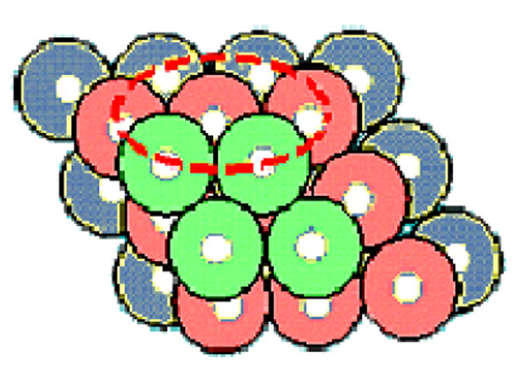
Packing of uniform-sized spheres in their highest density form. While amino acids do not pack exactly in this face-centered cubic lattice way, they do pack with similar angular preferences, but do not preserve the fixed distances between the centers of nearest neighbors.

Their angular distributions are preserved however, and actual residues pack with the angles shown in Fig. 2.

Fig. 2.

The angular positions occupied around a central residue within 6.5 Ǻ having 12 or more neighbors. Coloring is spectral with the highest densities shown in red. The numbers index the angular density maxima identified in Table 1.(13–15)

Residue points are taken as the C^β atoms and close residues within a radius of 6.8 Å are considered. Clusters obtained from a set of non-homologous protein structures were rotated to find an optimal superimposition. The central residue defines the origin of a spherical reference system with the rigid-body rotated directional vectors from different clusters intersecting the surface of a unit sphere. The most populous regions on the surface of this sphere define the most probable coordination directions, characterized by two spherical angles θ - polar, and φ - azimuthal. When there is less than a full set of neighbors, sites are gradually filled as the coordination number increases by clusters of nearby points. It is important to note that the filling is not sparse or staggered, but instead the relatively close sites are filled first, thus maintaining an approximately constant density excluding the solvent space. The optimal protein architecture can be viewed as a distorted, incomplete face centered cubic packing. This approximate cubic closest-packed geometry appears as a generic characteristic of the residue packing architecture for proteins. Note that face-centered cubic packing is the densest way to pack uniform spheres in space.

While these local orientation clusters are present in proteins, the ability to sustain substitutions of amino acids depends on other aspects of protein structure, such as the available space, its ability to accommodate side chains of a specific shape, the change in stabilizing interactions upon substitution. Thus it is difficult to make sense of individual substitutions. However, if we include a sufficiently large sample and average results, it becomes clearer as will be seen next.

2.1 Sequence alignments and structure

Employing sequence alignments in conjunction with molecular modeling has proven to provide significant improvements for protein structure prediction (18,19). One key assumption in homology-based modeling is that conserved regions share structural similarities, but the structural basis of this connection has not been clearly established. Although there have been many individual demonstrations of connections between sequence conservation and structural properties (20), there are no definitive studies on this subject. Establishing direct connections between sequences and structural features have proven difficult; hence the limited number of successes at protein design and the limited comprehension of mutagenesis. Recent applications that incorporate sequence variability into structure predictions have often lead to enhanced results (21), indicating that empirical measures of sequence variability are useful by themselves, even if their full implications are not well understood.

2.2 Sequence variability

Entropy is defined as the sum over the physical states i of a system, $-\sum _i{p}_{i}ln{p}_i$. Developing such a measure for the probabilities of individual residues at each place in a structure is straightforward, and these types of computed Shannon entropies for protein sequences have proven useful and have been shown to correlate with entropies calculated from local physical parameters, including backbone geometry (22). A deeper exploration of the connection between sequence entropy and protein structure is useful for developing a better understanding of protein stability and function.

While extending the investigations of packing in proteins for greater detail could prove to be informative, we have chosen to investigate the coarse-grained packing of the points representing neighboring amino acids similarly to what was developed in the previous section. The results we will see are quite general, even if not so immediately useful for protein structure predictions, and we have established a strong relationship between packing density and sequence conservation. Specifically we generate a large set of aligned protein sequences over a diverse sample of 130 non-redundant protein sequences, all having structures in the PDB, and calculate sequence entropies for each individual residue position in the alignment. These are then compared with a corresponding local flexibility as defined by the C^α packing density calculated from the corresponding structures. Similar comparisons can also be made between residue hydrophobicity and packing density.

Sequence alignments were generated using BLASTP (23) searching through GenBank available from the National Center of Biotechnology Information (NCBI, 2002). Alignments are not included if bit scores fall below 100 and they are required to be at a level greater than or equal to 40% of the best score. Exploratory calculations showed that 40% of the BLASTP bit score was a reasonable threshold for calculations of sequence entropy and its relationship with density. Also a minimal set of sequences is required, and a maximum number of 100 alignments are typically included. This yields a set of 7,143 aligned protein sequences. The average number of alignments per query is 55. The frequency distribution of the BLASTP bit scores for all 130 sets of alignments is consistent with the right-skewed (i.e. positive skew) distribution for a randomized set of BLAST scores (24). Here the mean, median and the overall range of BLASTP bit scores for all 7,143 alignments were 408, 354 and 100 to 1,793. Sequence entropy S_k at amino acid position k was calculated from

$$S_k=-\sum _{j=1.20}{p}_{jk}ln{p}_{jk}+\sum _{j=1.20}{p}_{j}ln{p}_j$$ (1)

where p_jk is the probability at some amino acid sequence position k derived from the frequency f_jk for an amino acid type j at sequence position k for all of aligned residues and p_j is the probability of amino acid type j in all alignments. Gaps were ignored. The second term corresponds to the random case, which has been subtracted (25). C^α packing densities are calculated from the atomic coordinates. The radius for inclusion in the packing calculation was 9 Å. Here we discuss the extent to which the inverse of this local packing density, as a measure of local flexibility (26), is correlated with sequence variability. Calculated sequence entropies for individual proteins when compared with the inverse C^α packing density do not agree with one another. For example three individual proteins gave slopes of the best fit lines of 13.0, 6.1 and 4.3. This appears to be because the sample sizes within individual proteins are insufficiently large. In our sample over the entire set of proteins there were a total of 41,543 residues. The results shown in Fig. 3(27) were first averaged for each protein and then averaged over the set of proteins within each interval of density.

Fig. 3.

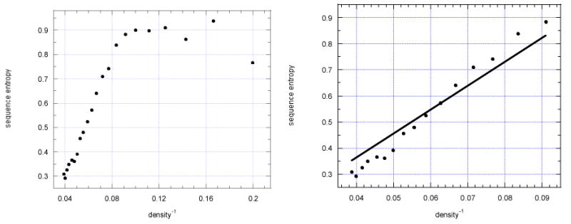
Relationship between sequence variability, expressed as sequence entropy and inverse residue packing density. These results are shown for a set of 113 proteins. Note that there are two different regions seen in the figure on the left - a nearly linear region for high packing densities and a more constant region for low packing densities. On the right the data for a broad range of the higher packing densities have been fit with a straight line (27).

There are two major regions corresponding to high and low densities visible in the correlation plots of sequence entropy versus inverse packing density. The first region for higher packing densities has a steep slope, and corresponds to densities of 12 to 25 C^α atoms (inverse densities from 0.040 to 0.083). There is the hint of a slight sigmoidal shape to the curve. The second region on the right of the figure includes a significant number of residues but appears to be nearly constant in sequence entropy; this region involves lower packing densities ranging from 6 to 11. It is quite logical that in the low packing density regime, changes in sequence entropy should be unaffected by their packing. The surprise is that there is constant sequence variability for the low residue packing density regime.

2.3 Flexibility and Hydrophobicity and Sequence Entropy

Previously a strong correlation was reported between computed displacements using elastic networks, which directly reflects residue packing (20,28) and the measured hydrogen exchange (HX). Regions of high packing density naturally resist hydrogen exchange, because of both stability and inaccessibility. Here, we have gone further to relate the calculated inverse C^α packing density from X-ray structures to sequence variability. Strong linear correlations are observed between sequence entropy and the inverse packing density, except for the lowest range of density. This provides a quantitative relationship between these two quantities, and can provide an important structural measure for determining likely non-disruptive sites for mutagenesis.

There is also a strong correlation between calculated sequence entropy and hydrophobicity. Clearly, correlations between the sequence variabilities as reflected in the sequence entropies, and the corresponding hydrophobicities are consistent with the average behavior for residues within a given packing density range. Still, this observed correlation between average sequence entropy and hydrophobicity is noteworthy, but both density and hydrophobicity are reflecting fundamental properties related to the extent of burial. The critical importance of hydrophobicity for folding of model protein chains (29,30) is well known. This is consistent with the fact that key hydrophobic residues can be described as buried or tightly packed (7–9). Packing and the resulting interactions associated with hydrophobicity were reported by Dima and Thirumalai (31) to be manifested in pairs and triplets of contacts. Our calculation of residue packing density represents a coarse-grained counting of such contacts. It is possible to calculate more detailed measures than those used here, by using full atomic representations. Such calculations would depend upon the residue's environment in more detailed ways, than is given by the present simple residue density. Progress in this direction could assist with protein design - a closely related problem (10,22,32–37). Further efforts are clearly required to achieve such a goal; however, the present results point the way towards such a goal. Here packing at the residue level for coarse-grained structures has been shown to exhibit an extremely strong connection to sequence conservation. Why is the averaging here necessary? One possible explanation is that the large number of combinatorial ways in which a group of residues' atoms can be packed together requires averaging over large numbers of occurrences, in order to obtain a meaningful single coarse-grained value.

3. Elastic Network Models

Originally, elastic network theory was developed for networks of polymer chains. James and Guth (38–44) developed in the forties a theory of a “phantom network” whose behavior is dictated only by the connectivity of the network chains if the effect of the excluded volume of polymer chains is neglected. The chains are phantom-like; i.e. they are able to pass readily through one another. They assumed that the network is composed of crosslinked Gaussian chains. They assumed that there are two types of network junctions. Junctions at the surface of the rubber are fixed and deform affinely with the macroscopic strain, while the junctions inside the network are free to fluctuate about their mean positions. The configurational partition function Z_N of the network is the product of the configurational partition functions of the individual Gaussian chains (45).

$$Z_N=C\prod _{i<j}exp[-\frac{1}{2}\sum _i\sum _j{\gamma }_{ij}{(R_i-R_j)}^2]$$ (2)

where R_i is the position of junction i, C is a normalization constant and the matrix elements γ_ij are defined as

$${\gamma }_{ij}=\{\begin{array}{cc}\frac{3}{2<r_{ij}^2>0}& \text{if i and j are connected by a chain}\\ 0& \text{if i and j are not connected}\end{array}$$ (3)

where <(r_ij)²>₀ is the mean square end-to-end vector of the chain between junctions i and j in the undeformed state. The diagonal elements are defined so that the summation of all matrix elements in a given row (or column) is zero.

$${\gamma }_{ii}=-\sum _j{\gamma }_{ij}$$ (4)

This means that all statistical properties of the network depend on the connectivity matrix Γ defined in Eqs. 3–4. One can easily calculate fluctuations of junctions in the phantom network model, and correlations between these fluctuations for the ideal infinite network with the topology of a tree (with network junctions having functionality φ - the number of chains connected at each junction). An example of such a tree-like network is shown in Fig. 4.

Fig.4.

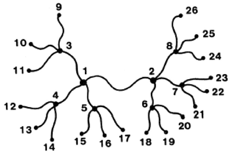
The first three tiers of a unimodal symmetrically grown tree-like network with functionality φ = 4. When this is applied to denatured proteins, these network connections will include both sequence (chain) connections and non-bonded interactions.

These quantities are related to the matrix elements of the inverse matrix Γ^-1. The mean square fluctuations of the end-to-end vector < (Δr)²> of polymer chains depend on the functionality φ of the network as

$$<{(\text{Δ}\text{r})}^2>=\frac{2}{\text{φ}}{<\text{r}}^{\text{2}}{>}_0$$ (5)

It can be shown that correlations <(ΔR_i·ΔR_j)> are related to Γ_ij^-1

$$<(\text{Δ}{\text{R}}_{\text{i}}·\text{Δ}{\text{R}}_{\text{j}})>=\frac{3}{2}{\text{Γ}}_{\text{ij}}^{-1}$$ (6)

The problem of fluctuations of junctions and chains in random phantom networks has been studied in detail by Kloczkowski, Mark and Erman (46,47). In the simplest case when junctions i and j are directly connected by a single chain the solution of the problem converges to the following simple formula

$$\left[\begin{array}{cc}<\text{(}\text{Δ}{\text{R}}_{\text{i}}{\text{)}}^{\text{2}}>& <\text{(}\text{Δ}{\text{R}}_{\text{i}}·\text{Δ}{\text{R}}_{\text{j}}\text{)}>\\ <\text{(}\text{Δ}{\text{R}}_{\text{i}}·\text{Δ}{\text{R}}_{\text{j}}\text{)}>& <\text{(}\text{Δ}{\text{R}}_{\text{j}}{\text{)}}^{\text{2}}>\end{array}\right]={<\text{r}}^2{>}_{\text{0}}\left[\begin{array}{l}\frac{\text{φ}-1}{\text{φ}(\text{φ}-2)}\frac{1}{\text{φ}(\text{φ}-2)}\\ \frac{1}{\text{φ}(\text{φ}-2)}\frac{\text{φ}-1}{\text{φ}(\text{φ}-2)}\end{array}\right]$$ (7)

where φ is the functionality of the network. In the case of two junctions m and n separated by d other junctions along the path joining m and n the solution of the problem is

$$\left[\begin{array}{cc}<{(\text{Δ}{\text{R}}_{\text{m}})}^2>& <(\text{Δ}{\text{R}}_{\text{m}}·\text{Δ}{\text{R}}_{\text{n}})>\\ <(\text{Δ}{\text{R}}_{\text{m}}·\text{Δ}{\text{R}}_{\text{n}})>& <{(\text{Δ}{\text{R}}_{\text{n}})}^2>\end{array}\right]=<{\text{r}}^{\text{2}}{>}_0\left[\begin{array}{cc}\frac{\text{φ}-\text{1}}{\text{φ}(\text{φ}-\text{2})}& \frac{1}{\text{φ}(\text{φ}-\text{2}){(\text{φ}-\text{1})}^{\text{d}}}\\ \frac{1}{\text{φ}(\text{φ}-\text{2}){(\text{φ}-\text{1})}^{\text{d}}}& \frac{\text{φ}-\text{1}}{\text{φ}(\text{φ}-\text{2})}\end{array}\right]$$ (8)

and the fluctuations <(Δr_mn)²> of the distance r_mn are

$$<\text{(}\text{Δ}{\text{r}}_{\text{mn}}{\text{)}}^{\text{2}}>=\frac{2}{\text{φ}(\text{φ}-2)(\text{d}+1)}\frac{{(\text{φ}-1)}^{\text{d}+1}-1}{{(\text{φ}-1)}^{\text{d}}}{<\text{r}}_{\text{mn}}^{\text{2}}{>}_0$$ (9)

The problem was also solved for the general case of fluctuations of points along the chains in the network and correlations of fluctuations among such points. To deal with this case it was assumed that each chain between two functional junctions is composed of n Gaussian segments connected by bifunctional junctions to form a chain, as shown in Fig. 5.

Fig. 5.

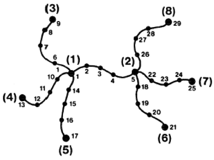
Tetrafuctional network with additional bifunctional junctions that separate each chain into four subchains of equal length. Such segments can ideally represent loops on the surfaces of proteins.

Because of this the diagonal elements γ_ii of the connectivity matrix are φ if the index i corresponds to the φ functional junction and 2 for the bifunctional junction. The off-diagonal elements γ_ij are −1 if i and j are directly connected by a chain segment, and zero otherwise. For the infinite number of tiers in the tree-like network the solution of the problem has the following form

$$\left[\begin{array}{cc}<\text{(}\text{Δ}{\text{R}}_{\text{i}}{\text{)}}^{\text{2}}>& <\text{(}\text{Δ}{\text{R}}_{\text{i}}·\text{Δ}{\text{R}}_{\text{j}}\text{)}>\\ <\text{(}\text{Δ}{\text{R}}_{\text{i}}·\text{Δ}{\text{R}}_{\text{j}}\text{)}>& <\text{(}\text{Δ}{\text{R}}_{\text{j}}{\text{)}}^{\text{2}}>\end{array}\right]={<\text{r}}^{\text{2}}{>}_{\text{0}}\left[\begin{array}{cc}\frac{\text{φ}-1}{\text{φ}(\text{φ}-2)}+\frac{\zeta (1-\zeta )(\text{φ}-2)}{\text{φ}}& \frac{1}{\text{φ}(\text{φ}-2){(\text{φ}-1)}^{\text{d}}}+\frac{\left[1+\zeta (\text{φ}-2)\right]\left[(\text{φ}-1)-\text{θ}(\text{φ}-2)\right]}{\text{φ}}\\ \frac{1}{\text{φ}(\text{φ}-2){(\text{φ}-1)}^{\text{d}}}+\frac{\left[1+\zeta (\text{φ}-2)\right]\left[(\text{φ}-1)-\text{θ}(\text{φ}-2)\right]}{\text{φ}}& \frac{\text{φ}-1}{\text{φ}(\text{φ}-2)}\frac{\text{θ}(1-\text{θ})(\text{φ}-2)}{\text{φ}}\end{array}\right]$$ (10)

where $\text{ζ}=\frac{\text{i}-1}{\text{n}}$ and $\text{θ}=\frac{\text{j}-1}{\text{n}}$ are the fractional distances of sites i and j from the nearest φ-functional junctions on their left side (as shown in Fig. 6) with 0 < ζ θ< 1, and d is the number of φ-functional junctions between sites i and j. Our preliminary results show that Eq. 10 is applicable also to proteins loops.

Fig. 6.

Two points i and j of the network separated by d = 3 tetrafunctional junctions. The positions of points i and j are measured with respect to the nearest multifunctional junction from the left as fractions ζ θ of the contour length of the chain between multifuctional junctions.

3.1 Elastic Network Models of Proteins - Gaussian Network Model

The EN models developed for polymer networks have been successfully applied to proteins in many different applications by us (20,48–68) and many others (53,54,69–92). The basic difference between elastomeric polymer networks and proteins is that a protein is a collapsed polymer with many non-bonded interactions, while for polymers these non-bonded interactions could be (as for the phantom chain models) completely neglected. The simplest EN model of proteins is the Gaussian Network Model (GNM). In the GNM it is assumed that fluctuations of residues about their mean positions are spherically symmetric. (The Anisotropic Network Model (ANM) discussed in the next section assumes that these fluctuations are represented by ellipsoids.) For the usual level of one point per amino acid, usually taken as the C^α atoms, all close points within a cutoff distance R_c are connected with identical deformable springs. While this is a kind of uniform material model of proteins, it provides a representation of the mechanics of the intact structure, and does not have the level of detail of a potential energy function that would be needed for describing the folding process or how the structure was arrived at. It is assumed that the initial structure (usually a well-resolved crystal structure) is lowest in energy. The energy of each spring increases with deviations ΔR away from the initial structure, with ΔR following a Gaussian distribution. The total energy of the network at is given by

$${\text{V}}_{\text{tot}}=\left(\gamma /2\right)\mathrm{ tr }\left[\text{Δ}{\text{R}}^{\text{T}} \text{Γ} \text{Δ}\text{R}\right]$$ (11)

where Γ is the Kirchhoff (contact) matrix defined on the basis of the cutoff distance R_c and tr is the trace of the matrix. Then the average changes in position, given either as the correlation between the displacements of pairs of residues i and j or as the mean-square fluctuations for a single residue i, are

$$<\text{Δ}{\text{R}}_{\text{1}}^{\text{2}}>=<\text{Δ}{\text{R}}_{\text{i}}·\text{Δ}{\text{R}}_{\text{i}}>=(1/{\text{Z}}_{\text{N}})\int (\text{Δ}{\text{R}}_{\text{i}}·\text{Δ}{\text{R}}_{\text{j}})\text{ exp }\left\{-{\text{V}}_{\text{tot}}/\text{kT}\right\}\text{ d}\left\{\text{Δ}\text{R}\right\}=(3\text{kT}/\text{γ}){\left[{\text{Γ}}^{-1}\right]}_{\text{ij}}$$ (12)

The most direct validation of this approach has been made by comparing the computed fluctuation magnitudes with the Debye-Waller temperature factors usually reported by crystallographers as B-factors

$${\text{B}}_{\text{i}}=8{\pi }^2<\text{Δ}{\text{R}}_{\text{i}}·\text{Δ}{\text{R}}_{\text{i}}>/3$$ (13)

Usually excellent agreement is achieved by this approach when B-factors of high resolution structures are compared. Another test was a comparison with H/D exchange data (64), where the protection factors and/or free energy of exchange from experiments for a series of proteins were closely reproduced/explained by the theoretical (GNM) results. Other tests (performed after mode-decomposition of GNM dynamics, see below) include a comparison of the most constrained regions in the GNM with conserved residues and/or folding nuclei, comparison of hinge sites (minima in the slowest mode fluctuation curve) and cross-correlations between domain motions, with those revealed in experimental studies.

The applicability of the GNM to oligonucleotides, or protein- RNA complexes is supported by our studies. Fig. 7 shows how the GNM methodology closely reproduces the experimental B-factors measured for tRNA in isolated form, and when bound to Gln synthetase.

Fig. 7.

Comparison of the computed (black) and experimental (red) temperature factors, for tRNA^Gln, with and without its cognate'. Notably the changes in nucleotide mobilities occurring upon binding of the tRNA to the protein are well reproduced by the GNM computations.

Another study that lends support to the use of the GNM is the application to HIV-1 reverse transcriptase (RT), where RTs in different forms (bound to DNA, or to inhibitors) were analyzed to infer the mechanism of action, consistent with experimental data (59,63,93).

3.2. Elastic Network Models of Proteins. Anisotropic Network Model

The GNM provides information on the sizes of fluctuations, <ΔR_i²>, and on their cross-correlations, <ΔR_i•ΔR_j>. The Anisotropic Network Model (ANM) is the extension that includes fluctuation vector directions (94). In the ANM, the potential is defined as a function of inter-residue distances R_ij as

$$V_2({\stackrel{\rho }{r}}_{ij})=\frac{1}{2}\gamma {\text{(}{R}_{\mathrm{ij}}-R_{\mathrm{ij}}^{\text{0}}\text{)}}^{\text{2}}H\text{(}{R}_c-R_{ij}\text{)}$$ (14)

where R_ij⁰ is the equilibrium (native state) distance between residues i and j, and H(x) is the Heaviside step function equal to 1 if x > 0, and zero otherwise. V can be rewritten as an expression similar in form to eq 13, where Γ is replaced by the 3N x 3N Hessian matrix H_ANM of the 2^nd derivatives of the potential with respect to positions, similar to classical normal mode analysis (NMA) of equilibrium structures. H_ANM provides information on the individual components, ΔX_i, ΔY_i, and ΔZ_i of the deformation vectors ΔR_i, and their correlations, whereas GNM yields only the magnitudes of ΔR_i and the correlations between ΔR_i vectors, only.

The contributions of the individual EN modes to the observed motion are found by eigenvalue decomposition of G(GNM) [or H(ANM)]. The individual eigenvectors represent the normal modes of motion. The decomposition is represented as Γ⁻¹ = Σ λ_κ⁻¹ [u_ku_k^T], where λ _κ is the k^th eigenvalue and u_k is the k^th eigenvector. Note that the solution requires using singular value decomposition to remove the zero eigenvalue terms corresponding to rigid-body translations and rotations in order to obtain the remaining eigenvalues and eigenvectors. In general, the result is a small number of modes that contribute most, and a large number that have only small contributions (95). This is consistent with the general viewpoint that proteins are highly cohesive materials, and that the collective motions, which correspond to domain-like motions, are the most related to function. The localized, high-frequency motions do not significantly contribute to the overall motions, but are perhaps related to stability (20,96). We note that the use of harmonic potentials restricts the amplitude of motions, and truly large transitions are not observed with the present EN models (87,88).

We have recently applied the ANM (94) to the ribosome (These results will be shown in detail in the last section). This and a recent study by another group (97), which also employs the ANM methodology, provide firm evidence for the utility and applicability of the EN models to represent and predict the dynamics of not only proteins, but also other biological structures such as protein-RNA complexes, and the ribosome.

3.3 Hierarchical levels of coarse-graining

The hypothesis is that the most cooperative (lowest frequency) modes of motion are insensitive to the details of the model and parameters, and can be satisfactorily captured by adopting low resolution EN models. Fig. 8 gives the results from an application (62) to two large proteins of the hierarchical coarse-graining scheme we have recently introduced (95), which support this hypothesis.

Fig. 8.

Motions of (A) influenza virus hemagglutinin A (HA) and (B) β– galactosidase (GAL), at different levels of detail. The top diagrams show the native structures, and the diagrams (a)–(d) show their ‘deformed’ conformations predicted by the ANM. Panels (a) and (b) show the ribbon diagram (left) and coarse-grained GNM representation (right) of deformed HA structures, induced by the slowest two collective modes of motion. Their counterparts for β-galactosidase are shown in panels (c) and (d). The coarse-grained models are constructed using m = 10, i.e. groups of 10 consecutive residues are condensed into unified nodes of the EN model (61–62, 95).

The idea is to adopt a low resolution EN representation, where each node stands for a group of m residues condensed into a single interaction site. Calculations performed for different levels of coarse-graining (m = 1, 2, 10, 40) have shown that the slowest modes of motion are preserved regardless of the level of coarse-graining. Part a) compares the slowest mode (a global torsion) predicted for influenza virus hemagglutinin A (HA) using EN models of m = 1 (left) and 10 (right). One of the monomers is shown in black for visualizing the motion. The two symmetric structures shown in each case refer to the ‘deformed’ conformations between which the original structure fluctuates, thus disclosing the potential global changes in structure favored by the equilibrium topology of inter-residue contacts. Part (b) shows the second most probable mode, a cooperative bending of the trimer. The functional implications of these modes have been discussed in our earlier study (28). Panel B shows similar results for β-galactosidase (GAL), confirming that the global motions of the system of N residues are almost identically reproduced by adopting a coarse-grained (m = 10, N/10 nodes) model.

The ANM computation time for a given structure scales with the 3^rd power of the number of EN nodes. The use of a model of N/10 sites would increase the computational speed by three orders of magnitude. Application of the hierarchical coarse-graining to HA showed that the global dynamics are accurately captured even with an EN model of only N/40 nodes. The change in the coordinates of every m^th residue is computed in this approach and by repeating this approach m times, each time shifting the selected node-residue by one residue along the sequence permits us to reconstruct the fluctuation profile of all N residues, with a net reduction in computation time by a factor of m².

3.4. Mixed coarse-graining

A mixed coarse-graining (MCG) approach (28) has also been introduced for EN models, where a protein's native conformation is represented by different regions having high and low resolution. The aim here is to capture the dynamics of the interesting parts in structures at higher resolution and retain the remainder of the structure at lower resolution. As a result, the total number of nodes in a system can be kept sufficiently low for computational tractability.

4. Modeling Ribosome Functional Dynamics

The X-ray crystal structure of the 30S subunit from the T. thermophilus was reported by Wimberly et al. (98). The crystal structure of the entire assembly of the 70S ribosome from T. thermophilus has been reported by Yusupov et al. (99). We performed ANM analysis on the structure of the 30S subunit reported from Wimberly et al. (PDB code 1J5E),the 50S subunit from Yusupov et al. (PDB code 1GIY) and the 70S ribosome structure reported by Yusupov et al.(99) (PDB structrues 1gix and 1giy). The 30S subunit of Wimberly et al. (98) contains full coordinates for the rRNAs, whereas the structure of the 70S ribosome by Yusupov et al. (99) contains only the P atoms of the rRNAs and the C^α atoms of the proteins, except for the three tRNAs and mRNA. The cutoff distance for interaction is taken as 15Ǻ. We used one interaction site on the P atom per nucleotide of the rRNAs and tRNAs and one interaction site on the C^α atom of the proteins. The cutoff distance between the C^α –C^α atoms is still 15Ǻ, but the cutoff distance between P-P and P-C^α atoms is increased to 24 Ǻ. The dimensions of the ANM contact matrices (equivalent to NMA Hessian) are 16,266 × 16,266 for the 30S subunit, and 29,238 × 29,238 for the 70S. We utilized the software BLZPACK of Marques and Sanejouand. (84). This yields a specific number of eigenvalues and eigenvectors for this matrix and is quite rapid.

4.1 ANM Results for the 50S subunit and the 70S assembly

Flexibility in the 50S subunit predicted by the ANM is illustrated in Fig. 9.

Fig 9.

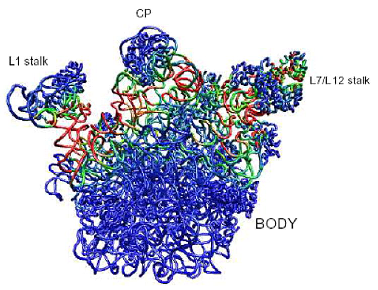
Structure of the 50S subunit color-coded according to the deformation energy averaged over the ten slowest (dominant) modes. The interfacial regions between these domains and the body is highly flexible, indicated by the high deformation energies found by ANM, and shown by the red-green portions above. This flexibility ensures the functional mobilities of the L1 stalk, CP and L7/L12 domains (48).

The figure displays the 50S subunit from T. thermophilus (PDB code: 1GIY), viewed from the 30S interface side. Residues are color-coded according to the deformation energy averaged over the ten slowest modes. The landmarks on the structures are: center protuberance (CP), L1 stalk, L7/L12 stalk and the body. There are four dynamic domains: L1 stalk, L7/L12 stalk, CP, and the body. The two stalks and the CP are found by GNM/ANM (not shown) to be highly mobile, and their relative motions oppose each other against the body for the first few slowest modes. For example, in mode 1, only the L1 stalk is mobile and it moves toward the CP. In mode 2, we see the L1 and L7/L12 stalks move out of the plane of the page, and the CP moves in the opposite direction. Motions of the 70S assembly in the slowest modes can be viewed in http://ribosome.bb.iastate.edu/70SnKmode/. The deformable residues are found to be located mostly at the interface between the two subunits, an indication that the two subunits form separate dynamic domains relative to each other. A recent study compared the differences between the atomic positions from low resolution cryo-EM density maps of the 70S ribosome in two different functional states (100–102) and reported that they were related by a ratchet-like motion, which is the type of motion we observe in several of the slowest modes of motion. In an additional experimental observation from cryo-EM the 30S subunit was observed to rotate counter-clockwise (viewed from the 30S solvent side) when EF-G binds, reducing the opening between the CP and L1 stalk and bifurcating the L7/L12 stalk. This motion was most similar to our computed mode 3. In this mode, when the two stalks pull toward the CP, the 30S subunit rotates counter-clockwise viewed from the 30S solvent side. The L7/L12 stalk also undergoes a large conformational change that may be linked to an observed bifurcation. The study of Tama et al. also reported that their mode 3 resembled the experimentally observed ratchet-like motion (103). However, we have seen a much more significant re-arrangement in the deformation of the L7/L12 stalk in this mode than they report. Another difference occurs for mode 1, where they have only the motion of the L1 stalk, whereas our mode 1 includes a counter-rotation of the two subunits and the motions of the two stalks.

Analysis of the motions of the structural subunits and their relative motions within the 70S ribosome give further information. Table 2 gives the orientation correlations between the motions of the ribosome structural units averaged over the 100 slowest modes.

Table 2. Correlations between the motions of ribosome structural units (48)^*.

	50S	A-tRNA	P-tRNA	E-tRNA	mRNA
30S	−0.99	−0.06	−0.10	−0.07	0.50
50S		−0.01	0.03	−0.01	−0.55
A-tRNA			0.77	0.17	0.42
P-tRNA				0.31	0.39
E-tRNA					0.19

^*from the ANM analysis of the PDB files:1GIX+1GIY.

The motions of the 30S and 50S subunits are almost perfectly anticorrelated (i.e. coupled but rotation in opposite directions).

This could arise from both the counter-rotation and from the opening-closing motions. Their motions are extremely weakly correlated with the tRNAs, because the tRNAs and the mRNA move linearly and in a direction tangential to the rotational motions of the 30S and 50S subunits. The 30S and mRNA are positively correlated, whereas the 50S and mRNA are anticorrelated. This indicates that the mRNA moves in the same direction as the 30S subunit, and in the opposite direction to the 50S subunit. In addition, the A-tRNA and the P-tRNA are strongly and positively correlated with each other, but they are less correlated with the E-tRNA. A strong correlation between the A-tRNA and the P-tRNA indicates that the A-tRNA and the P-tRNA move together in the same direction. This may indicate that the translocation of the A-tRNA to the P site and the translocation of the P-tRNA to the E site are likely to occur simultaneously. However, we see that the E-tRNA motion is not so strongly correlated with either the A-tRNA or P-tRNA, but nonetheless more strongly correlated with its neighboring P-site tRNA than with the A-site tRNA (48).

Fig. 10 shows the amplitudes of motions in the slowest modes, revealing the high mobility of the 50S and 30S subunits and the E site tRNA during the collective motions of the 70S assembly.

Fig. 10.

Amplitude of motions induced by the first seven slowest modes on 70S assembly subunits, averaged over residues forming these subunits. The 50S shows especially large displacements in the slowest two modes. The E-site tRNA exhibits large displacements in modes 3, 4, and 6. The distortion of the E tRNA in mode 4 is illustrated in the ribbon diagram on the right (leftmost yellow group). The order of the bars for each mode (left to right) is that given in the key (top to bottom) (48).

Analysis the deformation energies within each structural units reveal that the large mobility of the E-tRNA is mainly due to inter- subunit movements that relate to the exit of the E-tRNA from the assembly. Further analysis of the tRNA motions has revealed that the rigid body directions of their motions correspond closely to the directional vectors connecting the center of the tRNA to the center of its neighboring tRNA site (48). We anticipate learning further details of the mechanism of the ribosome by further analysis and application of the mixed coarse graining approach.

5. Summary

We have discussed the effects of residue packing density on protein structure and how these observations provide some justification for the EN models. The basic approaches used in these models originates in polymer theory where it has been shown possible to represent a variety of systems havinig different connectivities. These approaches outlined could, for example, be combined with the EN protein models to represent the disordered parts of proteins.

The EN models for proteins are robust and do not depend on the details of protein structure; consequently they can be applied to extremely large systems, which can be possible only by approximating structures with relatively highly coarse-grained models. We have shown the results of EN simulations on the ribosome, which compare favorably with the electron micrograph images of the ratchet motions in the ribosome. The correlated motions seen overall correspond closely to what would be expected for the functional processing steps of the ribosome.

Table 1.

Coordination states of surface to core central residues for groups of amino acids having different numbers of neighboring residues, m. Residues have neighbor coordination number of 3–4 are principally surface residues, all residue are included in 3 ≤ m ≤14 and core residues are represented by m ≥10, and residues having m ≥ 12 include the most densely packed residues. (13–15).

Coordination number		Coordination states (degrees)
		1	2	3	4	5	6	7	8	9	10	11	12
3 ≤ m≤ 4	θ	40	45			95	90
	φ	30	170			50	110
(3 ≤m≤14)	θ	40	35	45	95	105	55	90(b)					120
	φ	10	200	285	350	50	115	180(b)					115
m≥10	θ	45	45	45	95	105	60	100	85	105	140
	φ	40	180	280	360	60	100	140	240	300	220
m≥12	θ	45	25	50	70	100	75	80	75	105	140	145	130
	φ	60	170	280	340	40	120	160	220	260	200	330	120
fcc lattice	θ	35	35	35	90	90	90	90	90	90	145	145	145
	φ	30	150	270	360	60	120	180	240	300	210	330	90

References

- 1.Richards FM. The interpretation of protein structures: Total volume, group volume and packing density. J Mol Biol. 1974;82:1–14. doi: 10.1016/0022-2836(74)90570-1. [DOI] [PubMed] [Google Scholar]
- 2.Hermans J, Scheraga HA. Structural studies of ribonuclease. IV. Abnormal ionizable groups. J Am Chem Soc. 1961;83:3283–3292. [Google Scholar]
- 3.Richards FM. Protein stability: Still an unsolved problem. Cell Mol Life Sci. 1997;53:790–802. doi: 10.1007/s000180050100. [DOI] [PMC free article] [PubMed] [Google Scholar]
- 4.Liang J, Dill KA. Are proteins well-packed? Biophys J. 2001;81:751–766. doi: 10.1016/S0006-3495(01)75739-6. [DOI] [PMC free article] [PubMed] [Google Scholar]
- 5.Eriksson AE, Baase WA, Zhang XJ, Heinz DW, Blaber M, Baldwin EP, Matthews BW. Response of a protein structure to cavity-creating mutations and its relation to the hydrophobic effect. Science. 1992;255:178–183. doi: 10.1126/science.1553543. [DOI] [PubMed] [Google Scholar]
- 6.Privalov PL. Intermediate states in protein folding. J Mol Biol. 1996;258:707–725. doi: 10.1006/jmbi.1996.0280. [DOI] [PubMed] [Google Scholar]
- 7.Ptitsyn OB. Protein folding and protein evolution: Common folding nucleus in different subfamilies of c-type cytochromes? J Mol Biol. 1998;278:655–666. doi: 10.1006/jmbi.1997.1620. [DOI] [PubMed] [Google Scholar]
- 8.Ptitsyn OB, Ting KL. Non-functional conserved residues in globins and their possible role as a folding nucleus. J Mol Biol. 1999;291:671–682. doi: 10.1006/jmbi.1999.2920. [DOI] [PubMed] [Google Scholar]
- 9.Ting KL, Jernigan RL. Identifying a folding nucleus for the Lysozyme/alpha-lactalbumin family from sequence conservation clusters. J Mol Evol. 2002;54:425–436. doi: 10.1007/s00239-001-0033-x. [DOI] [PubMed] [Google Scholar]
- 10.Dahiyat BI, Mayo SL. De novo protein design: Fully automated sequence selection. Science. 1997;278:82–87. doi: 10.1126/science.278.5335.82. [DOI] [PubMed] [Google Scholar]
- 11.Mirny L, Abkevich VL, Shakhnovich EI. How evolution makes proteins fold quickly. Proc Natl Acad Sci U S A. 1998;95:4976–4981. doi: 10.1073/pnas.95.9.4976. [DOI] [PMC free article] [PubMed] [Google Scholar]
- 12.Solis AD, Rackovsky S. Optimally informative backbone structural propensities in proteins. Proteins. 2002;48:463–486. doi: 10.1002/prot.10126. [DOI] [PubMed] [Google Scholar]
- 13.Bagci Z, Kloczkowski A, Jernigan RL, Bahar I. The origin and extent of coarse-grained regularities in protein internal packing. Proteins. 2003;53:56–67. doi: 10.1002/prot.10435. [DOI] [PubMed] [Google Scholar]
- 14.Bagci Z, Jernigan RL, Bahar I. Residue packing in proteins: Uniform distribution on a coarse-grained scale. J Chem Phys. 2002;116:2269–2276. [Google Scholar]
- 15.Bagci Z, Jernigan RL, Bahar I. Residue coordination in proteins conforms to the closest packing of spheres. Polymer. 2002;43:451–459. [Google Scholar]
- 16.Jones DT. Protein structure prediction in the postgenomic era. Curr Opin Struct Biol. 2000;10:371–379. doi: 10.1016/s0959-440x(00)00099-3. [DOI] [PubMed] [Google Scholar]
- 17.Baker D, Sali A. Protein structure prediction and structural genomics. Science. 2001;294:93–96. doi: 10.1126/science.1065659. [DOI] [PubMed] [Google Scholar]
- 18.Bryant SH, Lawrence CE. An empirical energy function for threading protein sequence through the folding motif. Proteins. 1993;16:92–112. doi: 10.1002/prot.340160110. [DOI] [PubMed] [Google Scholar]
- 19.Marti-Renom MA, Stuart AC, Fiser A, Sanchez R, Melo F, Sali A. Comparative protein structure modeling of genes and genomes. Annu Rev Biophys Biomol Struct. 2000;29:291–325. doi: 10.1146/annurev.biophys.29.1.291. [DOI] [PubMed] [Google Scholar]
- 20.Demirel MC, Atilgan AR, Jernigan RL, Erman B, Bahar I. Identification of kinetically hot residues in proteins. Protein Sci. 1998;7:2522–2532. doi: 10.1002/pro.5560071205. [DOI] [PMC free article] [PubMed] [Google Scholar]
- 21.Kloczkowski A, Ting KL, Jernigan RL, Garnier J. Combining the GOR V algorithm with evolutionary information for protein secondary structure prediction from amino acid sequence. Proteins. 2002;49:154–166. doi: 10.1002/prot.10181. [DOI] [PubMed] [Google Scholar]
- 22.Koehl P, Levitt M. Protein topology and stability define the space of allowed sequences. Proc Natl Acad Sci U S A. 2002;99:1280–1285. doi: 10.1073/pnas.032405199. [DOI] [PMC free article] [PubMed] [Google Scholar]
- 23.Altschul SF, Madden TL, Scaffer AA, Zhang J, Zhang Z, Miller W, Lipman DJ. Gapped BLAST and PSI-BLAST: A new generation of protein database search programs. Nucleic Acids Res. 1997;25:3389–3402. doi: 10.1093/nar/25.17.3389. [DOI] [PMC free article] [PubMed] [Google Scholar]
- 24.Altschul SF, Boguski MS, Gish W, Wooten JC. Issues in searching molecular sequence databases. Nat Genet. 1994;6:119–129. doi: 10.1038/ng0294-119. [DOI] [PubMed] [Google Scholar]
- 25.Gerstein M, Altman RB. Average core structures and variability measures for protein families: Application to the immunoblobulins. J Mol Biol. 1995;251:161–175. doi: 10.1006/jmbi.1995.0423. [DOI] [PubMed] [Google Scholar]
- 26.Haliloglu T, Bahar I, Erman B. Gaussian dynamics of folded proteins. Phys Rev Lett. 1997;79:3090–3093. [Google Scholar]
- 27.Liao H, Yeh W, Chiang D, Jernigan RL, Lustig B. Protein sequence entropy is closely related to packing density and hydrophobicity. Protein Eng Des Sel. 2005;18:59–64. doi: 10.1093/protein/gzi009. [DOI] [PMC free article] [PubMed] [Google Scholar]
- 28.Bahar I, Atilgan AR, Demirel MC, Erman B. Vibrational dynamics of folded proteins: Significance of slow and fast motions in relation to function and stability. Phys Rev Lett. 1998;80:2733–2736. [Google Scholar]
- 29.Hinds DA, Levitt M. Exploring conformational space with a simple lattice model for protein structure. J Mol Biol. 1994;243:668–682. doi: 10.1016/0022-2836(94)90040-x. [DOI] [PubMed] [Google Scholar]
- 30.Dill KA, Bromberg S, Yue K, Fiebig KM, Yee DP, Thomas PD, Chan HS. Principles of protein folding: A perspective from simple exact models. Protein Sci. 1995;4:561–602. doi: 10.1002/pro.5560040401. [DOI] [PMC free article] [PubMed] [Google Scholar]
- 31.Dima RI, Thirmalai D. Asymmetry in the shapes of folded and denatured states of proteins. J Phys Chem B. 2004;108:6564–6570. [Google Scholar]
- 32.Li H, Tang C, Wingreen NS. Are protein folds atypical? Proc Natl Acad Sci U S A. 1998;95:4987–4990. doi: 10.1073/pnas.95.9.4987. [DOI] [PMC free article] [PubMed] [Google Scholar]
- 33.Buchler NE, Goldstein RA. Effect of alphabet size and foldability requirements on protein structure designability. Proteins. 1999;34:113–124. [PubMed] [Google Scholar]
- 34.Shih CT, Su ZY, Gwan JF, Hao BL, Hsieh CH, Lee HC. Mean-field HP model, designability and alpha-helices in protein structures. Phys Rev Lett. 2000;84:386–389. doi: 10.1103/PhysRevLett.84.386. [DOI] [PubMed] [Google Scholar]
- 35.Tiana G, Broglia RA, Provasi D. Designability of lattice model heteropolymers. Phys Rev E Stat Nonlin Soft Matter Phys. 2001;64:011904. doi: 10.1103/PhysRevE.64.011904. [DOI] [PubMed] [Google Scholar]
- 36.Larson SM, England JL, Desjarlais JR, Pande VS. Thoroughly sampling sequence space: Large-scale protein design of structural ensembles. Protein Sci. 2002;11:2804–2813. doi: 10.1110/ps.0203902. [DOI] [PMC free article] [PubMed] [Google Scholar]
- 37.England JL, Shakhnovich BE, Shakhnovich EI. Natural selection of more designable folds: A mechanism for thermophilic adaptation. Proc Natl Acad Sci U S A. 2003;100:8727–8731. doi: 10.1073/pnas.1530713100. [DOI] [PMC free article] [PubMed] [Google Scholar]
- 38.James HM, Guth E. Ind Eng Chem. 1941;33:624. [Google Scholar]
- 39.James HM, Guth E. Ind Eng Chem. 1942;34:1365. [Google Scholar]
- 40.James HM, Guth E. J Chem Phys. 1943;10:455–481. [Google Scholar]
- 41.James HM, Guth E. J Appl Phys. 1944;15:294–303. [Google Scholar]
- 42.James HM, Guth E. Theory of the Increase in Rigidity of Rubber During Cure. J Chem Phys. 1947;15:669–683. [Google Scholar]
- 43.James HM, Guth E. Simple Presentation of Network Theory of Rubber, with A Discussion of Other Theories. J Polym Sci. 1949;4:153–182. [Google Scholar]
- 44.James HM, Guth E. Statistical Thermodynamics of Rubber Elasticity. J Chem Phys. 1953;21:1039. [Google Scholar]
- 45.Flory PJ. Proc Roy Soc London. 1976;A351:351–380. [Google Scholar]
- 46.Kloczkowski A, Mark JE, Erman B. Chain dimensions and fluctuations in random elastomeric networks I. Phantom Gaussian networks in the undeformed state. Macromolecules. 1989;22:1423–1432. [Google Scholar]
- 47.Kloczkowski A, Mark JE, Erman B. The James-Guth Model in modern theories of neutron scattering from polymer networks. Comput Polym Sci. 1992;2:8–31. [Google Scholar]
- 48.Wang Y, Rader AJ, Bahar I, Jernigan RL. Global ribosome motions revealed with elastic network model. J Struct Biol. 2004;147:302–314. doi: 10.1016/j.jsb.2004.01.005. [DOI] [PubMed] [Google Scholar]
- 49.Sen TZ, Kloczkowski A, Jernigan RL, Yan C, Honavar V, Ho KM, Wang CZ, Ihm Y, Cao H, Gu X, Dobbs D. Predicting binding sites of hydrolase-inhibitor complexes by combining several methods. BMC Bioinformatics. 2004;5:205. doi: 10.1186/1471-2105-5-205. [DOI] [PMC free article] [PubMed] [Google Scholar]
- 50.Navizet I, Lavery R, Jernigan RL. Myosin flexibility: Structural domains and collective vibrations. Proteins. 2004;54:384–393. doi: 10.1002/prot.10476. [DOI] [PubMed] [Google Scholar]
- 51.Kurkcuoglu O, Jernigan RL, Doruker P. Mixed levels of coarse-graining of large proteins using elastic network model succeeds in extracting the slowest motions. Polymer. 2004;45:649–657. [Google Scholar]
- 52.Kundu S, Jernigan RL. Molecular mechanism of domain swapping in proteins: An analysis of slower motions. Biophys J. 2004;86:3846–3854. doi: 10.1529/biophysj.103.034736. [DOI] [PMC free article] [PubMed] [Google Scholar]
- 53.Kim MK, Jernigan RL, Chirikjian GS. An elastic network model of HK97 capsid maturation. J Struct Biol. 2003;143:107–117. doi: 10.1016/s1047-8477(03)00126-6. [DOI] [PubMed] [Google Scholar]
- 54.Kim MK, Chirikjian GS, Jernigan RL. Elastic models of conformational transitions in macromolecules. J Mol Graph Model. 2002;21:151–160. doi: 10.1016/s1093-3263(02)00143-2. [DOI] [PubMed] [Google Scholar]
- 55.Kim MK, Jernigan RL, Chirikjian GS. Efficient generation of feasible pathways for protein conformational transitions. Biophys J. 2002;83:1620–1630. doi: 10.1016/S0006-3495(02)73931-3. [DOI] [PMC free article] [PubMed] [Google Scholar]
- 56.Keskin O, Jernigan RL, Bahar I. Proteins with similar architecture exhibit similar large-scale dynamic behavior. Biophys J. 2000;78:2093–2106. doi: 10.1016/S0006-3495(00)76756-7. [DOI] [PMC free article] [PubMed] [Google Scholar]
- 57.Keskin O, Durell SR, Bahar I, Jernigan RL, Covell DG. Relating molecular flexibility to function: a case study of tubulin. Biophys J. 2002;83:663–680. doi: 10.1016/S0006-3495(02)75199-0. [DOI] [PMC free article] [PubMed] [Google Scholar]
- 58.Keskin O, Bahar I, Flatow D, Covell DG, Jernigan RL. Molecular mechanisms of chaperonin GroEL-GroES function. Biochemistry. 2002;41:491–501. doi: 10.1021/bi011393x. [DOI] [PubMed] [Google Scholar]
- 59.Jernigan RL, Bahar I, Covell DG, Atilgan AR, Erman B, Flatow DT. Relating the structure of HIV-1 reverse transcriptase to its processing steps. J Biomol Struct Dyn. 2000;11:49–55. doi: 10.1080/07391102.2000.10506603. [DOI] [PubMed] [Google Scholar]
- 60.Doruker P, Jernigan RL. Functional motions can be extracted from onlattice construction of protein structures. Proteins. 2003;53:174–181. doi: 10.1002/prot.10486. [DOI] [PubMed] [Google Scholar]
- 61.Doruker P, Jernigan RL, Bahar I. Dynamics of large proteins through hierarchical levels of coarse-grained structures. J Comput Chem. 2002;23:119–127. doi: 10.1002/jcc.1160. [DOI] [PubMed] [Google Scholar]
- 62.Doruker P, Jernigan RL, Navizet I, Hernandez R. Important fluctuation dynamics of large protein structures are preserved upon coarse-grained renormalization. Int J Quant Chem. 2002;90:822–837. [Google Scholar]
- 63.Bahar I, Erman B, Jernigan RL, Atilgan AR, Covell DG. Collective motions in HIV-1 reverse transcriptase: Examination of flexibility and enzyme function. J Mol Biol. 1999;285:1023–1037. doi: 10.1006/jmbi.1998.2371. [DOI] [PubMed] [Google Scholar]
- 64.Bahar I, Wallqvist A, Covell DG, Jernigan RL. Correlation between native-state hydrogen exchange and cooperative residue fluctuations from a simple model. Biochemistry. 1998;37:1067–1075. doi: 10.1021/bi9720641. [DOI] [PubMed] [Google Scholar]
- 65.Bahar I, Jernigan RL. Cooperative fluctuations and subunit communication in tryptophan synthase. Biochemistry. 1999;38:3478–3490. doi: 10.1021/bi982697v. [DOI] [PubMed] [Google Scholar]
- 66.Atilgan AR, Durell SR, Jernigan RL, Demirel MC, Keskin O, Bahar I. Anisotropy of fluctuation dynamics of proteins with an elastic network model. Biophys J. 2001;80:505–515. doi: 10.1016/S0006-3495(01)76033-X. [DOI] [PMC free article] [PubMed] [Google Scholar]
- 67.Kim MK, Jernigan RL, Chirikjian GS. Rigid-Cluster Models of Conformational Transitions in Macromolecular Machines and Assemblies. Biophys J. 2005 doi: 10.1529/biophysj.104.044347. in press. [DOI] [PMC free article] [PubMed] [Google Scholar]
- 68.Bahar I, Jernigan RL. Vibrational dynamics of transfer RNAs: Comparison of the free and synthetase-bound forms. J Mol Biol. 1998;281:871–884. doi: 10.1006/jmbi.1998.1978. [DOI] [PubMed] [Google Scholar]
- 69.Zheng W, Doniach S. A comparative study of motor-protein motions by using a simple elastic-network model. Proc Natl Acad Sci U S A. 2003;100:13253–13258. doi: 10.1073/pnas.2235686100. [DOI] [PMC free article] [PubMed] [Google Scholar]
- 70.Zheng W, Brooks B. Identification of dynamical correlations within the myosin motor domain by the normal mode analysis of an elastic network model. J Mol Biol. 2005;346:745–759. doi: 10.1016/j.jmb.2004.12.020. [DOI] [PubMed] [Google Scholar]
- 71.Van Wynsberghe A, Li G, Cui Q. Normal-mode analysis suggests protein flexibility modulation throughout RNA polymerase's functional cycle. Biochemistry. 2004;43:13083–13096. doi: 10.1021/bi049738+. [DOI] [PubMed] [Google Scholar]
- 72.Tirion MM. Large amplitude elastic motions in proteins from a single-parameter, atomic analysis. Phys Rev Lett. 1996;77:1905–1908. doi: 10.1103/PhysRevLett.77.1905. [DOI] [PubMed] [Google Scholar]
- 73.Temiz NA, Meirovitch E, Bahar I. Escherichia coli adenylate kinase dynamics: Comparison of elastic network model modes with mode-coupling (15)N-NMR relaxation data. Proteins. 2004;57:468–480. doi: 10.1002/prot.20226. [DOI] [PMC free article] [PubMed] [Google Scholar]
- 74.Tama F, Brooks CL., III Diversity and identity of mechanical properties of icosahedral viral capsids studied with elastic network normal mode analysis. J Mol Biol. 2005;345:299–314. doi: 10.1016/j.jmb.2004.10.054. [DOI] [PubMed] [Google Scholar]
- 75.Tama F, Wriggers W, Brooks CL., III Exploring global distortions of biological macromolecules and assemblies from low-resolution structural information and elastic network theory. J Mol Biol. 2002;321:297–305. doi: 10.1016/s0022-2836(02)00627-7. [DOI] [PubMed] [Google Scholar]
- 76.Tama F, Miyashita O, Brooks CL., III Flexible multi-scale fitting of atomic structures into low-resolution electron density maps with elastic network normal mode analysis. J Mol Biol. 2004;337:985–999. doi: 10.1016/j.jmb.2004.01.048. [DOI] [PubMed] [Google Scholar]
- 77.Micheletti C, Lattanzi G, Maritan A. Elastic properties of proteins: Insight on the folding process and evolutionary selection of native structures. J Mol Biol. 2002;321:909–921. doi: 10.1016/s0022-2836(02)00710-6. [DOI] [PubMed] [Google Scholar]
- 78.Li G, Cui Q. Analysis of functional motions in Brownian molecular machines with an efficient block normal mode approach: Myosin-II and Ca2+ −ATPase. Biophys J. 2004;86:743–763. doi: 10.1016/S0006-3495(04)74152-1. [DOI] [PMC free article] [PubMed] [Google Scholar]
- 79.Kong Y, Ming D, Wu Y, Stoops JK, Zhou ZH, Ma J. Conformational flexibility of pyruvate dehydrogenase complexes: A computational analysis by quantized elastic deformational model. J Mol Biol. 2003;330:129–135. doi: 10.1016/s0022-2836(03)00555-2. [DOI] [PubMed] [Google Scholar]
- 80.Delarue M, Sanejouand YH. Simplified normal mode analysis of conformational transitions in DNA-dependent polymerases: The elastic network model. J Mol Biol. 2002;320:1011–1024. doi: 10.1016/s0022-2836(02)00562-4. [DOI] [PubMed] [Google Scholar]
- 81.ben Avraham D, Tirion MM. Dynamic and elastic properties of F-actin: A normal-modes analysis. Biophys J. 1995;68:1231–1245. doi: 10.1016/S0006-3495(95)80299-7. [DOI] [PMC free article] [PubMed] [Google Scholar]
- 82.Valadie H, Lacapcre JJ, Sanejouand YH, Etchebest C. Dynamical properties of the MscL of Escherichia coli: A normal mode analysis. J Mol Biol. 2003;332:657–674. doi: 10.1016/s0022-2836(03)00851-9. [DOI] [PubMed] [Google Scholar]
- 83.Sanejouand YH. Normal-mode analysis suggests important flexibility between the two N-terminal domains of CD4 and supports the hypothesis of a conformational change in CD4 upon HIV binding. Protein Eng. 1996;9:671–677. doi: 10.1093/protein/9.8.671. [DOI] [PubMed] [Google Scholar]
- 84.Marques O, Sanejouand YH. Hinge-bending motion in citrate synthase arising from normal mode calculations. Proteins. 1995;23:557–560. doi: 10.1002/prot.340230410. [DOI] [PubMed] [Google Scholar]
- 85.Reuter N, Hinsen K, Lacapere JJ. The nature of the low-frequency normal modes of the E1Ca form of the SERCA1 Ca2+−ATPase. Ann N Y Acad Sci. 2003;986:344–346. doi: 10.1111/j.1749-6632.2003.tb07210.x. [DOI] [PubMed] [Google Scholar]
- 86.Hinsen K, Reuter N, Navaza J, Stokes DL, Lacapere JJ. Normal mode-based fitting of atomic structure into electron density maps: Application to sarcoplasmic reticulum Ca-ATPase. Biophys J. 2005;88:818–827. doi: 10.1529/biophysj.104.050716. [DOI] [PMC free article] [PubMed] [Google Scholar]
- 87.Hinsen K, Thomas A, Field MJ. Analysis of domain motions in large proteins. Proteins. 1999;34:369–382. [PubMed] [Google Scholar]
- 88.Hinsen K. Analysis of domain motions by approximate normal mode calculations. Proteins. 1998;33:417–429. doi: 10.1002/(sici)1097-0134(19981115)33:3<417::aid-prot10>3.0.co;2-8. [DOI] [PubMed] [Google Scholar]
- 89.Hinsen K, Thomas A, Field MJ. A simplified force field for describing vibrational protein dynamics over the whole frequency range. J Chem Phys. 1999;111:10766–10769. [Google Scholar]
- 90.Beuron F, Flynn TC, Ma J, Kondo H, Zhang X, Freemont PS. Motions and negative cooperativity between p97 domains revealed by cryo-electron microscopy and quantised elastic deformational model. J Mol Biol. 2003;327:619–629. doi: 10.1016/s0022-2836(03)00178-5. [DOI] [PubMed] [Google Scholar]
- 91.Ming D, Kong Y, Lambert MA, Huang Z, Ma J. How to describe protein motion without amino acid sequence and atomic coordinates. Proc Natl Acad Sci U S A. 2002;99:8620–8625. doi: 10.1073/pnas.082148899. [DOI] [PMC free article] [PubMed] [Google Scholar]
- 92.Ming D, Kong Y, Wakil SJ, Brink J, Ma J. Domain movements in human fatty acid synthase by quantized elastic deformational model. Proc Natl Acad Sci U S A. 2002;99:7895–7899. doi: 10.1073/pnas.112222299. [DOI] [PMC free article] [PubMed] [Google Scholar]
- 93.Temiz NA, Bahar I. Inhibitor binding alters the directions of domain motions in HIV-1 reverse transcriptase. Proteins. 2002;49:61–70. doi: 10.1002/prot.10183. [DOI] [PubMed] [Google Scholar]
- 94.Atilgan AR, Durell SR, Jernigan RL, Demirel MC, Keskin O, Bahar I. Anisotropy of fluctuation dynamics of proteins with an elastic network model. Biophysical Journal. 2001;80:505–515. doi: 10.1016/S0006-3495(01)76033-X. [DOI] [PMC free article] [PubMed] [Google Scholar]
- 95.Doruker P, Jernigan RL, Bahar I. Dynamics of large proteins through hierarchical levels of coarse-grained structures. Journal of Computational Chemistry. 2002;23:119–127. doi: 10.1002/jcc.1160. [DOI] [PubMed] [Google Scholar]
- 96.Bahar I, Atilgan AR, Demirel MC, Erman B. Vibrational dynamics of folded proteins: Significance of slow and fast motions in relation to function and stability. Physical Review Letters. 1998;80:2733–2736. [Google Scholar]
- 97.Tama F, Valle M, Frank J, Brooks CL., III Dynamic reorganization of the functionally active ribosome explored by normal mode analysis and cryo-electron microscopy. Proc Natl Acad Sci U S A. 2003;100:9319–9323. doi: 10.1073/pnas.1632476100. [DOI] [PMC free article] [PubMed] [Google Scholar]
- 98.Wimberly BT, Brodersen DE, Clemons WM, Jr, Morgan-Warren RJ, Carter AP, Vonrhein C, Hartsch T, Ramakrishnan V. Structure of the 30S ribosomal subunit. Nature. 2000;407:327–339. doi: 10.1038/35030006. [DOI] [PubMed] [Google Scholar]
- 99.Yusupov MM, Yusupova GZ, Baucom A, Lieberman K, Earnest TN, Cate JH, Noller HF. Crystal structure of the ribosome at 5.5 A resolution. Science. 2001;292:883–896. doi: 10.1126/science.1060089. [DOI] [PubMed] [Google Scholar]
- 100.Tama F, Valle M, Frank J, Brooks CL., III Dynamic reorganization of the functionally active ribosome explored by normal mode analysis and cryo-electron microscopy. Proc Natl Acad Sci U S A. 2003;100:9319–9323. doi: 10.1073/pnas.1632476100. [DOI] [PMC free article] [PubMed] [Google Scholar]
- 101.Agrawal RK, Spahn CM, Penczek P, Grassucci RA, Nierhaus KH, Frank J. Visualization of tRNA movements on the Escherichia coli 70S ribosome during the elongation cycle. J Cell Biol. 2000;150:447–460. doi: 10.1083/jcb.150.3.447. [DOI] [PMC free article] [PubMed] [Google Scholar]
- 102.Frank J, Agrawal RK. A ratchet-like inter-subunit reorganization of the ribosome during translocation. Nature. 2000;406:318–322. doi: 10.1038/35018597. [DOI] [PubMed] [Google Scholar]
- 103.Tama F, Valle M, Frank J, Brooks CL., III Dynamic reorganization of the functionally active ribosome explored by normal mode analysis and cryo-electron microscopy. Proc Natl Acad Sci U S A. 2003;100:9319–9323. doi: 10.1073/pnas.1632476100. [DOI] [PMC free article] [PubMed] [Google Scholar]