Stability of Spectro-Temporal Tuning over Several Seconds in Primary Auditory Cortex of the Awake Ferret

Abstract

The steady-state spectro-temporal tuning of auditory cortical cells has been studied using a variety of broad-band stimuli that characterize neurons by their steady-state responses to long duration stimuli, lasting from about a second to several minutes. Central sensory stations are thought to adapt in their response to stimuli presented over extended periods of time. For instance, we have previously shown that auditory cortical neurons display a second order of adaptation, whereby the rate of their adaptation to the repeated presentation of fixed alternating stimuli decreases with each presentation. The auditory grating (or ripple) method of characterizing central auditory neurons, and its extensions, have proven very effective. But these stimuli are typically used with spectro-temporal content held fixed over time-scales of seconds, introducing the possibility of rapid adaptation while the receptive field is being measured, whereas the neural response used to compute a spectro-temporal receptive field (STRF) assumes stationarity in the neural input/output function. We demonstrate dynamic changes in some parameters during the measurement of the STRF over a period of seconds, even absent of a relevant behavioral task. Specifically, we find small but systematic changes in duration and breadth of tuning of STRFs when comparing the early (0.25 sec - 1.75 sec) and late (4.5 sec - 6 sec) segments of the responses to these stimuli.

Introduction

The use of broadband sounds to characterize neural responses in the auditory pathway is well established. Several classes of stimuli have been developed to characterize cells in primary auditory cortex (Schreiner and Calhoun, 1994, Kowalski et al., 1996a, deCharms et al., 1998, Miller and Schreiner, 2000, Blake and Merzenich, 2002, Machens et al., 2004, Valentine and Eggermont, 2004). In particular, neural responses to the presentation of auditory gratings, which are well-structured broadband sounds whose spectro-temporal envelopes vary sinusoidally in (log) spectrum and in time, can be used to generate a Spectro-Temporal Receptive Field (STRF) through reverse correlation techniques. Using gratings of varying periodicities in both spectral and temporal axes, the neural encoding of dynamic spectral envelopes can be jointly characterized in these two dimensions. In addition to providing a characterization of the input-output transformation carried out by the auditory neuron being analyzed, the resultant STRF can be used to predict the neural response to the same and to novel stimuli (Kowalski et al., 1996b).

As an extension to this method, Klein et. al. (2000) showed that this method of characterization can be used with composite stimuli, or Temporally Orthogonal Ripple Combinations (TORCs), which are sums of auditory gratings. This result required only the constraint that each of the component gratings in a TORC have a unique temporal periodicity, i.e., the component gratings were modulated distinctly in time. With the assumption of linearity, the neural response to each component grating was of the same periodicity as the grating. Therefore, the composite response to the TORC was separable by Fourier methods into the responses to each grating. Since multiple gratings were being presented concurrently, the obvious advantage of this method is in its reduction of the time necessary to characterize a neuron. We implement this method of characterization in the current study.

In this paper, cells in primary auditory cortex (AI) of awake ferrets (Mustela putorius furo) were adequately characterized by a set of grating stimuli with evenly spaced spectral densities and temporal angular frequencies. The typical range of spectral densities and angular frequencies that must be spanned in order to sufficiently probe an AI neuron’s response properties is known. However, given the non-deterministic nature of neural responses, the number of periods needed in order to get an estimate of the underlying probability density function governing neural firing is not a priori known. Given that the stimuli used are periodic, the duration of any sound can be extended until the characterization of the response for that stimulus is sufficiently stable.

Implementation of these sounds and other similar stimuli are of relatively long duration—generally seconds to minutes, and their spectro-temporal content is either fixed or changes slowly during the presentation. However, neurons in the central part of sensory pathways are thought to adapt in their responses to stimuli presented over extended periods of time. For instance, we have previously shown that neurons in AI display a second order of adaptation, whereby the characteristics of their adaptation to the continuous presentation of alternating long-duration grating stimuli, that differ in their modulation depth, changes with each step-change in the modulation depth (Shechter and Depireux, 2006). Computation of the STRF—and its subsequent usage in predicting responses—assumes a time-invariant system, in other words stationary response properties.

Evoked potentials typically contain multiple components, some lasting up to several seconds (Wang et al., 2006). In this study, we test the assumption of the cell’s receptive field being stationary throughout the sound presentation used to characterize the cell. We apply previously described methods to characterize neurons in AI, but derive two receptive fields from the responses we obtain—which we call early and late STRFs. These STRFs are computed from two distinct time windows of the responses, the epoch closely following the onset of the sounds we use to measure STRFs, and an epoch a few seconds later, at which point the evoked potentials related to the sound onset have died out. Namely, the early STRF is computed from responses to the first fourth of the stimulus (0.25 - 1.75 sec), and we compare it to the late STRF, which is computed from responses to the last fourth of the stimulus (4.5 - 6 sec).

It is known that adaptation of neural output is not restricted to occur only in response to changes in the mean value of the input. For instance, neurons in the early visual pathway also adapt in response to changes in the variance (contrast) of input signals (Smirnakis et al., 1997), and neurons in the auditory pathway adapt to changes in the kurtosis (a higher moment statistics of the modulation envelope, (Kvale and Schreiner, 2004)). Adaptation has been shown to occur along different stations of the visual pathway, from the retina (Baccus and Meister, 2002) to primary visual cortex (Crowder et al., 2006) and higher (Kohn and Movshon, 2004). In this paper, we analyze the stability of the steady-state characterization of primary auditory cortical cells in response to sounds several seconds in duration.

Methods

Surgical Procedures

Recordings were made from 6 awake, 3 to 12 month old, domestic ferrets (Mustela putorius furo) surgically implanted with chronic moveable multi-electrode arrays. A detailed description can be found in (Dobbins et al., 2007). Briefly, ferrets were anesthetized with Halothane (3% induction, 1.75% maintenance adjusted to keep heart rate, end-tidal CO2 and SpO2 within limits), and affixed within a stereotaxic frame. Body temperature was maintained at 37.5°C with a feedback heating pad. The scalp was incised rostro-caudally along the midline from bregma to the nuchal crest. The temporalis muscles were partially resected bilaterally. 8 stainless steel screws were inserted around the skull to anchor the subsequent headpost, custom multi-electrode microdrive, and dental cement used to fix the experimental apparatus. A headpost was positioned rostrally over the skull. A craniotomy was made unilaterally (usually on the left) or bilaterally, over AI. To prevent regrowth, the mitotic inhibitor 5-fluorouracil (5-FU) was applied (Spinks et al.). The microdrive was slowly lowered into position, and affixed with dental cement. The microdrive was previously loaded with 6 to 12 independently adjustable micro-electrodes (12Drive-H, Neuralynx, Tucson AZ), with a custom made piece, resting on the edges of the craniotomy, to lower the electrodes in a honeycomb pattern over AI in such a way that the minimum distance between adjacent electrodes was 225μm. The experimental apparatus and headpost were fixed in place with additional dental cement. After surgery, the ferrets were given Banamine (1mg/kg) and Baytril (.2 mg/kg) for three recovery days before recording began. All surgical and experimental procedures were approved by the University of Maryland Animal Care and Use Committee and were in accord with NIH Guidelines on the care and use of laboratory animals.

Neural Recordings

Recording sessions took place inside a double-walled sound booth (IAC, Bronx, NY, Noise Isolation Class of 70dB). The ferret was placed in a comfortable holder, with its head fixed using the implanted headpost to ensure the animal stayed within the calibrated sound field and to minimize movement noises. The animal was monitored through a closed-circuit video, and treats (e.g., Ferretone) were given between stimulus presentations to preserve wakefulness, as deemed needed from the emergence of monitored slow-wave activity.

Recording sessions typically lasted 4-6 hours. Neural activity was recorded with parylene-coated tungsten microelectrodes (initial impedance 3-6 MΩ at 1 kHz, shaft diameter 76 μm, Micro Probe, Inc, Gaithersburg, MD). Electrodes were individually advanced by manually turning a screw (156μm per turn). All recordings were marked with the depth relative to when spikes were first detected upon lowering the electrode bundle. Spike events were obtained by a simple level-crossing, set low enough to capture all spikes and usually some excursions of the evoked potential. Event times were assigned to the peak of the waveform with a resolution of 100 μsec or 125 μsec, depending on the session. The signal was bandpass filtered with low and high cutoff frequencies of 300Hz and 3kHz, respectively. After a recording session, events were sorted into classes using a modification of the MClust package (MClust, A. D. Redish), with the automated cluster cutter KlustaKwik (Harris and Redish, 2002) which uses a CEM algorithm (Conditional Expectation Maximization) for which we use the Fourier transform, first and second principal components and energy of each event to classify spikes. Our threshold for event detection was set low such that we would have a large class of events we could reject as not being measurements of a neural spike. For an event to be classified as a neural spike, we required bi- or tri-phasic waveforms, with small variance, clear separationg from neighboring cluster, and uniform presence throughout the duration of the recording session.

Stimulus Generation and Sound Presentation

All stimuli were generated digitally in MATLAB (Natick, MA), with custom software written by us, converted to an analog voltage (TDT RX6, Tucker David-Technologies, Alachua, FL) at 100kHz sampling rate, processed with an analog attenuator (TDT PA5), amplified (Crown DX-70) and then presented free field from an overhead speaker (Manger Transducer, Manger, Germany) located 1m at zenith relative to the animal’s head. The sound field was calibrated and equalized so as to obtain a flat response from the loudspeaker to within 1.5dB, at the location of the animal’s head.

Stimulus Set

STRFs were measured with a set of Temporally Orthogonal Ripple Combinations (TORC) stimuli which were each 6 seconds in duration and 7 octaves in bandwidth (Klein et al., 2000, Depireux et al., 2001). As mentioned earlier, the TORC stimuli are the sum of periodic auditory gratings—also called ripples—each having a spectro-temporal profile modulated sinusoidally in spectrum and in time. The modulation of a grating is characterized in spectrum by its spectral density Ω (cycles/octave), in time by its periodicity or angular frequency ω (Hz), and in amplitude by its excursions away from the mean level of the stimulus (modulation depth ΔA, % of mean). Each of the grating components that make up a TORC has the same spectral density and depth, but differs in angular frequency, thus sampling a set of points in spectro-temporal parameter space with a single, complex sound.

The TORC stimulus is built up from 100 component tones per octave. The amplitude S(x,t) of each component tone of frequency f, x = log₂ (f/f₀) and f₀ the lower edge of the spectrum, is adjusted at time t as

$$S(x,t)=L[1+\Delta A\cdot {\Sigma }_i\cos (2\pi (\Omega \cdot x+w_i\cdot t)+{\varphi }_i)],$$ (1)

for a linear modulation. S defines the spectro-temporal envelope of the stimulus. L is the average level of the stimulus (measured as the RMS of the stimulus with reference to a 1kHz sine tone) and φ_i are the starting phases of each of the component gratings in the TORC. Since the tones that make up a grating are logarithmically spaced, the TORC does not elicit the perception of a pitch. φ_i ’s in Eq.1 are “optimized”, in the sense that their values are changed by a random search in parameter space until a set of φ_i ’s are found that minimize the peakiness of the envelope, as measured by the peak to RMS ratio. Note that when both Ω and w are positive, the corresponding grating envelope travels towards the low frequencies.

Computation of STRFs

The derivation of the steady state STRF from TORC stimuli is now standard and will not be repeated here in full (Klein et al. 2000). Briefly, a reverse correlation method with the stimulus spectro-temporal envelope is used to obtain the STRF from the spike trains elicited by the stimulus. For each stimulus in the set, we generated another stimulus with an inverted spectro-temporal envelope (effectively, +ΔA is replaced by -ΔA in Eq.1) so as to compensate for even-order non-linearities such as induced by half-wave rectification. In order to allow the responses to reach a steady-state, the analysis was started 250 msec following the onset of each stimulus, thereby removing the effect of level transients present at the onset of the stimulus. By dividing the response into four equal length segments, two STRFs were constructed using 1.5 sec segments of the response: the first was taken early in the response (early STRF: from 0.25 sec to 1.75 sec) and the second was taken later in the response (late STRF: from 4.5 sec to 6 sec).

SNR Computation

To determine the reliability of the STRF measured for the steady state response, we computed a signal-to-noise ratio (SNR) of the corresponding modulation transfer function (MTF, the 2-dimensional Fourier transform of the STRF). The MTF is the dual representation of the STRF, where each (Ω, w) point is a complex number which represents the response of the neuron to an auditory grating with spectral density Ω (cycles/octave) and angular frequency ω (Hz), see Eq.1. The amplitude of the complex number is the corresponding amplitude of the response and the phase is the corresponding phase lag between stimulus and response. 100 bootstrap estimates ψ(Ω, w) were generated for each point of the MTF. Each ψ(Ω, w) is an estimate of the MTF derived by choosing periods, with repetition, from the set of neural responses. The SNR of each point (SNR_Ω,w) was taken to be the average power divided by the variance of the estimates. The SNR of the STRF was computed as the power-weighted mean of the SNR at each (Ω, w) point. P_{Ω, w} is the power of the MTF at the point (Ω, w).

$${\mathrm{SNR}}_{\Omega ,w}=\frac{\mid \sum _{\text{bootstraps}}\psi (\Omega ,w)\mid }{{\sigma }_{\psi }^2}$$ (2)

$$\mathrm{SNR}=\frac{\sum _{\Omega ,w}{P}_{\Omega ,w}\cdot {\mathrm{SNR}}_{\Omega ,w}}{\sum _{\Omega ,w}{P}_{\Omega ,w}}$$ (3)

Only receptive fields which had an SNR > 0.5 for both the early and late time segments were included in the later analyses. There were no cells for which the early SNR was below 0.5 and the late SNR was above 0.5, and conversely.

STRF Measures

We extracted several descriptive measures of the STRF features which allow us to quantify how those features evolve during the presentation of the TORC stimuli:

1. The peak spiking rate (the maximal value of the STRF).

2. The latency and duration of the STRF excitatory feature. The STRF latency was taken to be the delay at which the STRF attained its peak value, and the duration of the excitatory feature was computed to be the width at 50% of the peak value along the temporal cross-section containing the peak. (Fig. 1, #1 and #3)

3. The best frequency (BF) and bandwidth of the STRF excitatory feature. The BF was taken to be the frequency for which the STRF attained its peak value, and its bandwidth was computed to be the width at 50% of the peak value along the spectral cross-section containing the peak. (Fig. 1, #5 and #7)

4. The STRF envelope peak latency and duration. We computed the envelope of the temporal cross-section containing the peak of the STRF by taking the absolute value of its Hilbert transform. Its latency and duration were computed analogously to the measures computed in (2), only using the envelope and its peak. (Fig. 1, #2 and #4)

5. The STRF envelope peak frequency and bandwidth. We computed the envelope of the spectral cross-section containing the peak of the STRF by taking the absolute value of its Hilbert transform. The envelope peak frequency and bandwidth were then extracted from the envelope as in (3). (Fig. 1, #6 and #8)

6. The total power (P).

   $$P=\sum _x\sum _{\tau }{\mid \mathit{STRF}(x,\tau )\mid }^2$$ (4)

Figure 1. STRF Measures.

This figure shows an example STRF with an excitatory center and mildly asymmetric inhibitory surround. The temporal and spectral cross-sections are plotted above and to the left of the STRF, respectively. The cross-sections of the STRF envelope are represented by the dashed line plotted with the STRF cross-sections. The STRF temporal (1-4) and spectral (5-8) measures are shown by their corresponding numbers on the cross-sections. The STRF is in spikes/(sec·1) and is computed per full (100% = 1) modulation.

MTF Measures

Several parameters have been developed to characterize MTFs (and their corresponding STRFs) and can be directly applied in the current situation (Depireux et al., 2001). Specifically, calling Ω > 0, w > 0 quadrant 1 and Ω < 0, w > 0 quadrant 2:

1. The breadth of tuning (α_b) is a measure of how the power is spread around the center of mass of the absolute value of the MTF in each quadrant. The center of mass is computed in the standard fashion, where each point in the MTF is weighted by its power. If the cell’s tuning sharpens (or broadens), α_b will decrease (or increase), respectively:

   $${\alpha }_b=\sum _i\sum _j{P}_{{\Omega }_i,w_j}\cdot \sqrt{{\left(\frac{{\Omega }_i-{\Omega }_{\mathit{CM}}}{{\Omega }_{\max }}\right)}^2+{\left(\frac{w_j-w_{\mathit{CM}}}{w_{\max }}\right)}^2}$$ (5)

   where P_Ω,w is the power of modulation in response to a grating of (Ω, w) characteristics, or in other words the square of the amplitude of the (Ω, w) component of the MTF; (Ω_CM, w_CM) is the MTF center of mass in that quadrant, and (Ω_max, w_max) are the maximum spectral density and angular frequency tested, respectively.
2. The degree of inseparability (α_SVD). We decompose each MTF into a sum of separable functions by singular value decomposition (SVD). The SVD method is now standard and is explained in detail in (Abdi, 2007). Briefly, the singular value decomposition of a matrix produces a diagonal matrix Λ of the same dimension, with nonnegative diagonal elements λ_i ’s in decreasing order, and unitary matrices U and V so that U×Λ×V^T is the original matrix. Specifically, SVD decomposes the MTF as

   $$\begin{array}{c}\mathit{MTF}=U\cdot \Lambda \cdot V^T,\Lambda =\mathit{diag}({\lambda }_1,{\lambda }_2,\dots ,{\lambda }_n),{\lambda }_i>{\lambda }_{i+1}\hfill \\ \mathit{MTF}(\Omega ,w)=\sum _i{\lambda }_i{G}_i\left(\Omega \right)F_i\left(w\right)\hfill \end{array}$$ (6)
   Note that the columns of U are independent functions G_i of spectral density Ω, and the columns of V are independent functions F_i of angular frequency ω. We define

   $${\alpha }_{\mathit{SVD}}=\left(1-{\lambda }_1^2/\left(\sum _i{\lambda }_i^2\right)\right)$$ (7)

   α_SVD is therefore a measure of how much of the total MTF power is accounted for by the first singular vector. A value of 0 corresponds to a fully separable MTF, whereas values approaching 1 indicate an increasing level of inseparability.
3. The degree of direction selectivity (α_d). We measure P₁, the total power in the first quadrant of the MTF (responses to down-moving gratings), and P₂, the total power in the second quadrant of the MTF (responses to up-moving gratings), and compute α_d as:

   $${\alpha }_d=\frac{P_1-P_2}{P_1+P_2}$$ (8)

   A value of 0 indicates equal power in the two quadrants and therefore, no overall preference for up vs. down moving spectral envelopes. An absolute value of 1 indicates that all the power is contained in one quadrant, i.e. the cell is highly selective for direction of motion and responds only to up or down moving spectral envelopes.

4. The asymmetry of the spectral (α_s) and temporal (α_t) transfer functions around Ω = 0 and w = 0, respectively. To further quantify the up vs. down asymmetry, we introduce these two indices, α_s and α_t, which quantify how the asymmetry of the transfer functions arises with respect to the down-moving (quadrant 1) versus the up-moving (quadrant 2) components of the spectro-temporal envelope of sounds. We compute the cross correlation

   $${\alpha }_s=1-\mid \frac{\sum _{\Omega >0}{G}_1\left(\Omega \right)\cdot G_2^{\ast }(-\Omega )}{\sqrt{\sum _{\Omega >0}{\mid G_1\left(\Omega \right)\mid }^2\cdot \sum _{\Omega >0}{\mid G_2(-\Omega )\mid }^2}}\mid$$ (9)

   $${\alpha }_t=1-\mid \frac{\sum _{w>0}{F}_1\left(w\right)\cdot F_2^{\ast }\left(w\right)}{\sqrt{\sum _{w>0}{\mid F_1\left(w\right)\mid }^2\cdot \sum _{w>0}{\mid F_2\left(w\right)\mid }^2}}\mid$$ (10)

   where F and G are the temporal and spectral functions of the MTF quadrants respectively, and the subscripts 1,2 indicate the quadrant for which they are computed. Values near 0 correspond to symmetric transfer functions, whereas values near 1 correspond to asymmetry of the corresponding spectral or temporal transfer function. It has previously been shown that steady state STRFs in AI of the ferret are by and large quadrant separable and temporally symmetric (Simon et al., 2007).

5. The center of mass of tuning (Ω_CM, w_CM). Complementing the sharpness of tuning, we analyze the spectral densities and angular frequencies which elicit the best responses. The center of mass is computed in the standard fashion, where each point in the MTF is weighted by its power.

6. The spectral density and angular frequency bandwidths. We extract the absolute value of the spectral and temporal transfer functions for each quadrant of the MTF. The bandwidths are measured at 75% the value of the peak.

We extracted these measures for both the early and late STRFs. In order to assess whether there was a significant change between the values, we compared the measures of each STRF with a paired t-test. A significance threshold of p < 0.02 was used.

Results

Proximity to neural activity was recognized online during the recording session by monitoring the activity through an oscilloscope and an audio monitor. Neural activity corresponding to the auditory environment was first confirmed by responses to pure tone pips. TORC stimuli were then presented to acquire STRFs. Full analysis of the early (0.25 sec - 1.75 sec) and late (4.5 sec - 6 sec) segments of the responses to the TORCs was conducted offline, and only cells for which both early and late had an SNR which was greater than 0.5 were kept for further analysis. Since our measures are centered on the peak of the excitatory features of the STRF, we rejected 8 cells from our analysis which were primarily inhibited, i.e. most of the STRF was made up of a large negative feature. In all, we retained 78 cells.

Figure 2 demonstrates the nature of the changes we measured between the early and late STRFs. Fig. 2A demonstrates an STRF which changed in the time period over which it was acquired. For Cell 216, the feature of the late STRF (top right) is both longer in duration and spans a narrower bandwidth when compared to the early STRF (top left). For Cell 160 (Fig. 2B) there is no significant difference between early and late STRFs.

Figure 2. Typical Early and Late STRFs.

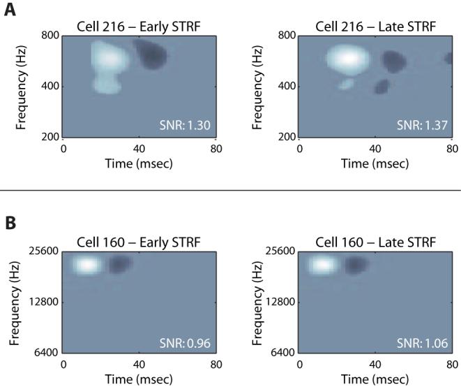
A, Cell 216 demonstrates the type of changes we see from early (left) to late (right) times in the responses to TORC stimuli. The excitatory feature of this cell is longer in duration and narrower in bandwidth in the late STRF when compared to the early STRF. B, Cell 160 shows a cell for which no changes were observed between early and late time periods.

Magnitude Measures

We first compared the SNR of the early and late STRFs. This allowed us to assess whether the reliability of the response changed with increasing the presentation duration. The SNR did not change significantly between the two conditions (Fig. 3C). Therefore, subsequent measures of the two conditions were directly comparable, and would not be influenced by a change in the reliability of responses. While the overall power in the STRF did not change significantly between the early and the late STRF (Fig. 3B), the peak value generally increased, with a sample mean increase of 2.8% (p<0.02) (Fig. 3A). α_b, which measures how power is spread in the MTF, did not change significantly between the two epochs. Two related power measures, α_SVD and α_d, which measure the degree of inseparability and the degree of direction selectivity, respectively, were also shown not to change significantly from earlier to later times in the response (Fig. 3D-F).

Figure 3. STRF Magnitude Measures.

A, There was a significant difference between the peak magnitude of the early STRF when compared to the late STRF, with a mean increase of 2.8% across the entire population (p<0.02). B-F, There were no significant changes between the early and late STRFs with respect to the total power, SNR, the degree of inseparability α_SVD, the degree of direction selectivity α_d, and the sharpness of tuning α_b. STRF Peak and Power are computed per full (100%) modulation.

Temporal Measures

The latency to the peak of the STRF corresponds to the lag between the occurrence of modulation at the cells best frequency to the correponding modulation in neural response it evokes or to the peak of its envelope. With increasing stimulus time, the latency did not change significantly (Fig. 4A). However, the duration of the excitatory feature (peak) increased by 4.8% (p<0.02) from early to late, corresponding to a longer duration in which the cell responds to modulation at its best frequency (Fig. 4B). This change was also reflected in the envelope of the STRF feature, which became wider, but did not reach significance. Analogously, the center of mass of the MTF shifted to smaller angular frequencies by 1% (Fig. 4D); this trend, however, only approached significance (p = 0.09). The angular frequency bandwidth of the MTF did not change significantly (Fig. 4C). Finally, there was no significant difference between values of the temporal symmetry measure α_t for the early or the late STRFs (Fig. 4E). It is interesting to note that 91% of cells had values of α_t which were smaller than 0.4 for both time periods, in good agreement with (Simon et al., 2007).

Figure 4. Temporal Measures.

A-B, While the latency to the excitatory peak of the STRF did not change between early and late STRFs, there was a significant increase in the peak’s duration by 4.8% (p<0.02). However, neither the latency nor duration of the STRF envelope changed significantly (data not shown). C,E, There were no significant differences between early and late STRFs measured by the bandwidth of angular frequencies (taken at 75% of the peak of the MTF spectral transfer function and the asymmetry of the MTF temporal transfer function. D, However, there was a 1% decreasing trend in the MTF angular frequency center of mass which was approaching significance (p=0.09).

Spectral Measures

Between the two analysis conditions, the BF of the STRF (the frequency at which the peak of the STRF occurred) did not change significantly (Fig. 5A). However, the bandwidth, which was measured at half the peak value along the spectral cross-section of the STRF corresponding to its latency, decreased by 5.2% (p<0.02) from the early STRF to the late STRF (corresponding to a narrower range of frequencies which elicit responses when modulated) (Fig. 5B). As was the case for the temporal measures, the corresponding STRF envelope measures for peak frequency and bandwidth did not change significantly. Reflecting the change in bandwidth, the center of mass of the MTF shifted to larger spectral densities by 3.3% (p<0.02) (Fig. 5D); in contrast to the angular frequency shift, this was a significant change. With the shift in center of mass, the spectral density bandwidth remained unchanged from early to late time periods in the response (Fig. 5C). No significant changes were observed for values of the spectral asymmetry index α_s (Fig. 5E).

Figure 5. Spectral Measures.

A, There was no significant difference between the best frequency measured in the early STRF and that measured in the late STRF. B, The bandwidth of the excitatory feature decreased (with a mean decrease of 5.2%) from the early to late STRFs (p<0.02). C, No significant differences between early and late STRFs were measured by the bandwidth of the MTF spectral transfer function. D, The MTF spectral density center of mass increased with a mean of 3.3% (p<0.02). E, There were no significant changes in the asymmetry of the MTF spectral transfer function between early and late STRFs.

Discussion

We have shown that receptive fields obtained using sounds lasting several seconds show a systematic change in the duration and bandwidth of their excitatory peaks. The remaining measures examined here remained stable.

Relation Between STRF and MTF measures

The analysis conducted in this paper includes measures pertaining to the STRF and its two-dimensional transform, the MTF. Since these are two dual spaces, there are corollaries of the findings with regards to the STRF in the MTF measures, and vice versa. Our main observation is that when the latter part of the responses to TORC stimuli is analyzed, the excitatory feature is longer in duration and narrower in spectrum as compared to analysis of the earlier part of those same responses. This effect could be mirrored by changes in the MTF in a number of ways. Ultimately, these changes would involve a shift of power in the MTF towards lower angular frequencies and higher spectral densities. In accord with this, we find that the center of mass of the late MTF shifts to lower angular frequencies and higher spectral densities, without a change in the spread of power around the center of mass (as measured by α_b). That α_b did not significantly change was confirmed by measurements of the angular frequency and spectral density bandwidths, which do not change significantly from early to late epochs.

Magnitude of Changes

The changes we see in the STRF are small in magnitude (e.g., 4.8% for duration, 5.2% for bandwidth). However, these changes are reliable in the population, and therefore constitute a significant effect. At the same time, many measures characterizing the response on average remain unchanged from earlier to later times during the stimulus presentation. This suggests that long duration sounds (on the order of 6 sec, as presented in this study) produce sufficiently stable responses for most applications of the STRF. This being said, it is important to note that the SNR-which is a measure of the reliability of observed responses-remains unchanged in the early and late epochs. This suggests that prolonged acquisition of data does not improve (but also does not deteriorate) our results significantly. This also implies that the optimal number of sound presentations should be obtained from an on-line continuous estimation of the SNR reaching a stable value.

We also compare these early and late SNRs to the SNR measured from the entire duration of the stimulus. There is not a significant change between either early or late SNR to the full SNR, suggesting that responses are equally reliable at all times during the stimulus presentation. Since in electrophysiological experiments, stimulus presentation time is a valuable resource, this has strong implications. Shorter duration sounds should be sufficient for characterizing the response properties of neurons in primary auditory cortex; of course, this does not preclude from the use of longer durations either. Given that the STRF is used to characterize the steady-state properties of neurons, it is important to know how steady the steady-state properties are. On the other hand, when using short duration sounds of the order of seconds, the analysis is started after the first period (250 msec) following the onset of each stimulus. During this initial time, the tuning is still stabilizing to the content of the stimulus. Our study shows that the use of stimuli that last several seconds is generally justified. Therefore time can be gained by the use of these longer sounds and minimizing the rejected response time during which neurons stabilize their tuning (in contrast to using multiple presentations of shorter stimuli).

Inhibitory STRFs

The majority of our neurons have the “classical” STRF, with a main excitatory feature and an inhibitory surround which is smaller in magnitude. With the SNR criterion used in this paper, 8 cells (about 10%) displayed an STRF for which the main feature is a prominently inhibited region. For these 8 cells, the peak of the absolute value of the STRF corresponded to an inhibitory region of the STRF. In all 8 cases, the STRF displayed either a large inhibitory region followed by a smaller excitation, or only inhibition. Correspondingly, the cells’ inhibitory region was very broadly tuned over several octaves, and all showed some level of direction selectivity. The particular, unique, features of these inhibitory STRFs requires a separate analysis; however, their small number precludes the feasibility of a statistical analysis and therefore they were not included the dataset.

Plasticity vs. Adaptive Changes

The changes we observed in the STRFs were in naïve listeners, with no behavioral paradigm. Previous literature has examined the dynamics of auditory cortical neurons (Irvine, 2007, Weinberger, 2007), and in particular the changes in STRFs associated a listening task after training: in particular, Fritz et. al. (2005) reported a temporal sharpening of the excitatory peak of the STRF and a commensurate increase in angular frequency in the MTF center of mass, by measuring the response of a sequence of sounds made up of TORCs similar to the ones used here, interspersed with a target pure tone. The experiments are quite different since they show a change in STRF properties following several minutes of behavioral response, whereas we show systematic changes over a few seconds of continuous sound presentation, change which resets itself between sound presentations. We note that the magnitude of the observed changes are opposite in direction between their plasticity and our adaptation experiments. We further note that the observed effect (except for the sign) are on the same order as the magnitude although we obtain ours without the introduction of a behavioral task during the sound presentation.

In conclusion, we show that spectro-temporal tuning, as measured by the STRF or its dual, the MTF, is relatively stable over several seconds, although a few parameters change in a systematic way. While details should depend on the intended application of the STRF, the appropriate method of characterization, and in particular sounds of appropriate durations, should be used.

Abbreviations

AI

Primary auditory cortex

MTF

modulation transfer function

STRF

spectro-temporal receptive field

TORC

temporally orthogonal ripple combination

References

- Abdi H. Singular Value Decomposition (SVD) and Generalized Singular Value Decomposition (GSVD) In: Salkind NJ, editor. Encyclopedia of Measurement and Statistics. Sage; Thousand Oaks, CA: 2007. [Google Scholar]
- Baccus SA, Meister M. Fast and slow contrast adaptation in retinal circuitry. Neuron. 2002;36:909–919. doi: 10.1016/s0896-6273(02)01050-4. [DOI] [PubMed] [Google Scholar]
- Blake DT, Merzenich MM. Changes of AI receptive fields with sound density. J Neurophysiol. 2002;88:3409–3420. doi: 10.1152/jn.00233.2002. [DOI] [PubMed] [Google Scholar]
- Crowder NA, Price NS, Hietanen MA, Dreher B, Clifford CW, Ibbotson MR. Relationship between contrast adaptation and orientation tuning in V1 and V2 of cat visual cortex. J Neurophysiol. 2006;95:271–283. doi: 10.1152/jn.00871.2005. [DOI] [PubMed] [Google Scholar]
- deCharms RC, Blake DT, Merzenich MM. Optimizing sound features for cortical neurons.[see comment] Science. 1998;280:1439–1443. doi: 10.1126/science.280.5368.1439. [DOI] [PubMed] [Google Scholar]
- Depireux DA, Simon JZ, Klein DJ, Shamma SA. Spectro-temporal response field characterization with dynamic ripples in ferret primary auditory cortex. Journal of Neurophysiology. 2001;85:1220–1234. doi: 10.1152/jn.2001.85.3.1220. [DOI] [PubMed] [Google Scholar]
- Dobbins HD, Marvit P, Ji YD, Depireux DA. Chronically Recording with a Multi-Electrode Array Device in the Auditory Cortex of an Awake Ferret. J Neurosci Meth. 2007:159. doi: 10.1016/j.jneumeth.2006.10.013. [DOI] [PMC free article] [PubMed] [Google Scholar]
- Fritz J, Elhilali M, Shamma S. Active listening: task-dependent plasticity of spectrotemporal receptive fields in primary auditory cortex. Hearing Research. 2005;206:159–176. doi: 10.1016/j.heares.2005.01.015. [DOI] [PubMed] [Google Scholar]
- Harris K, Redish AD. KlustaKwik and MClust-3.3. 2002. [Google Scholar]
- Irvine DR. Auditory cortical plasticity: Does it provide evidence for cognitive processing in the auditory cortex? Hear Res. 2007 doi: 10.1016/j.heares.2007.01.006. [DOI] [PMC free article] [PubMed] [Google Scholar]
- Klein DJ, Depireux DA, Simon JZ, Shamma SA. Robust spectrotemporal reverse correlation for the auditory system: optimizing stimulus design. Journal of Computational Neuroscience. 2000;9:85–111. doi: 10.1023/a:1008990412183. [DOI] [PubMed] [Google Scholar]
- Kohn A, Movshon JA. Adaptation changes the direction tuning of macaque MT neurons. Nat Neurosci. 2004;7:764–772. doi: 10.1038/nn1267. [DOI] [PubMed] [Google Scholar]
- Kowalski N, Depireux DA, Shamma SA. Analysis of dynamic spectra in ferret primary auditory cortex. I. Characteristics of single-unit responses to moving ripple spectra. Journal of Neurophysiology. 1996a;76:3503–3523. doi: 10.1152/jn.1996.76.5.3503. [DOI] [PubMed] [Google Scholar]
- Kowalski N, Depireux DA, Shamma SA. Analysis of dynamic spectra in ferret primary auditory cortex. II. Prediction of unit responses to arbitrary dynamic spectra. Journal of Neurophysiology. 1996b;76:3524–3534. doi: 10.1152/jn.1996.76.5.3524. [DOI] [PubMed] [Google Scholar]
- Kvale MN, Schreiner CE. Short-term adaptation of auditory receptive fields to dynamic stimuli. Journal of Neurophysiology. 2004;91:604–612. doi: 10.1152/jn.00484.2003. [DOI] [PubMed] [Google Scholar]
- Machens CK, Wehr MS, Zador AM. Linearity of cortical receptive fields measured with natural sounds. Journal of Neuroscience. 2004;24:1089–1100. doi: 10.1523/JNEUROSCI.4445-03.2004. [DOI] [PMC free article] [PubMed] [Google Scholar]
- Miller LM, Schreiner CE. Stimulus-based state control in the thalamocortical system. Journal of Neuroscience. 2000;20:7011–7016. doi: 10.1523/JNEUROSCI.20-18-07011.2000. [DOI] [PMC free article] [PubMed] [Google Scholar]
- Schreiner CE, Calhoun BM. Spectral envelope coding in cat primary auditory cortex:Properties of ripple transfer functions. Aud Neurosci. 1994;1:39–61. [Google Scholar]
- Shechter B, Depireux DA. Response Adaptation to Broadband Sounds in Primary Auditory Cortex of the Awake Ferret. Hearing Research. 2006;221:91–103. doi: 10.1016/j.heares.2006.08.002. [DOI] [PubMed] [Google Scholar]
- Simon JZ, Depireux DA, Klein DJ, Fritz JB, Shamma SA. Temporal symmetry in primary auditory cortex: implications for cortical connectivity. Neural computation. 2007;19:583–638. doi: 10.1162/neco.2007.19.3.583. [DOI] [PubMed] [Google Scholar]
- Smirnakis SM, Berry MJ, Warland DK, Bialek W, Meister M. Adaptation of retinal processing to image contrast and spatial scale. Nature. 1997;386:69–73. doi: 10.1038/386069a0. [DOI] [PubMed] [Google Scholar]
- Spinks RL, Baker SN, Jackson A, Khaw PT, Lemon RN. Problem of dural scarring in recording from awake, behaving monkeys: a solution using 5-fluorouracil. J Neurophysiol. 2003;90:1324–1332. doi: 10.1152/jn.00169.2003. [DOI] [PubMed] [Google Scholar]
- Valentine PA, Eggermont JJ. Stimulus dependence of spectro-temporal receptive fields in cat primary auditory cortex. Hear Res. 2004;196:119–133. doi: 10.1016/j.heares.2004.05.011. [DOI] [PubMed] [Google Scholar]
- Wang T, Ozdamar O, Bohorquez J, Shen Q, Cheour M. Wiener filter deconvolution of overlapping evoked potentials. Journal of neuroscience methods. 2006;158:260–270. doi: 10.1016/j.jneumeth.2006.05.023. [DOI] [PubMed] [Google Scholar]
- Weinberger NM. Auditory associative memory and representational plasticity in the primary auditory cortex. Hear Res. 2007 doi: 10.1016/j.heares.2007.01.004. [DOI] [PMC free article] [PubMed] [Google Scholar]