Dynamical Evolution of Spatiotemporal Patterns in Mammalian Middle Cortex

Abstract

The spatiotemporal structure of brain oscillations are important in understanding neural function. We analyze oscillatory episodes from isotropic preparations from the middle layers of mammalian cortex which display irregular and chaotic spatiotemporal wave activity, within which spontaneously emerge spiral and plane waves. The dimensionality of these dynamics show a consistent decrease during the middle of these episodes, regardless of the presence of simple spiral or plane waves. It is important to define the relevant biological order parameters which govern these dynamical bifurcations.

Neural systems think through patterns of activity. Recent work in primate cortex reinforces the growing evidence that aspects of cortical motor control and information transfer may need to be understood with respect to spatiotemporal patterns of oscillatory activity [1]. In human seizures, spatiotemporal patterns have been shown to have a consistent dynamical evolution as the seizure episodes initiate, develop, and terminate [2]. We have recently discovered that in an isotropic preparation of tangential slices of the middle cortical layers of mammalian brain, that spontaneously organizing episodes of activity also demonstrate a dynamical evolution: such episodes initiate with irregular and chaotic wave activity, followed by the frequent emergence of plane and spiral waves, and terminate with the recurrence of irregular wave patterns [3]. The spirals have true drifting phase singularities, behavior replicated in mean field continuum models of cortex [3]. An example of sequential experimental optical images of voltage sensitive dye response from such an experiment are shown in Fig 1.

Figure 1.

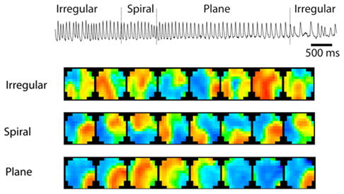
Example of oscillatory episode from middle cortical layers. Upper trace reflects a time series from a single photodetector within the array (extracellular microelectrode recordings follow a nearly identical pattern). Below this trace are sequences of optical frames from the different qualitative regimes (each row has 15 ms interframe interval from images collected at 1 kHz, imaging field 5 mm diameter). Spectral colormap proportional to voltage dye absorbance.

Nevertheless, understanding pattern formation in nonlinear systems outside of equilibrium remains a largely open problem [4]. We find that the analogy of such brain pattern formation with patterns from fluid turbulence is striking. Accordingly, we have explored techniques drawn from experimental fluid dynamics to better understand these phenomena. In voltage sensitive dye imaging from fields of neurons, we have applied an empirical eigenfunction approach, using singular value decomposition (SVD), f (t, x) = UΣV^T , where f (t, x) represents a matrix of sequential spatial values from the detectors measuring the average transmembrane potentials from the volume of neurons beneath each detector, U and V represent matrices of columnar orthogonal bases in time (u_i) and space (v_i), respectively, Σ indicates a diagonal matrix of singular values (σ_i), and T represents transpose [5]. The singular values weight the spatial eigenmodes v_i, and ${\sigma }_i^2$ would be proportional to the kinetic energy of v_i were it derived from a velocity field of an incompressible fluid. Each v_i has a time evolution in a corresponding u_i, and together they track the evolution of the coherent structures that comprise the full dynamics. The v_i are the statistically most likely spatial basis upon which to project the dynamics [6]. Indeed, one can often identify in turbulent systems that the overwhelming amount of energy expressed in this basis is found within a significantly confined region of the total phase space [7].

For long datasets the computation can become intractable. One greatly simplifies such analysis by collapsing time, for instance, by left multiplying by f (t, x)^T

$$f{(t,x)}^{T}f(t,x)=\mathbf{V}\mathrm{\Sigma }{\mathbf{U}}^T\mathbf{U}\mathrm{\Sigma }{\mathbf{V}}^T$$

and subsequently right multiplying by V, f^T f V = VΣ² , creating an eigenvalue problem from the correlation matrix f^T f and its eigenvector V, and then solving for U [6]

$$\mathbf{U}=f(t,x)\mathbf{V}{\mathrm{\Sigma }}^{-1}$$

One can examine the trajectories of the u_i to visually inspect changes in the dynamical complexity as the episodes evolve. Such a technique was used by [8] in examination of wave formation in turtle cortex.

We here analyze data from 500 μm thick slices from the visual cortex of rats [9] stained with the absorbance voltage sensitive dye NK3630, and with exposure to carbachol and bicuculline to activate the neurons and remove inhibition respectively (full details on experimental preparation are in [3]). We select 13 experiments collected on separate days for detailed dynamical study, chosen because the recording captured with minimal artifact a complete oscillatory episode. We archive essential code and a data sample in [10].

We first form a new SVD on every 1 sec of data (1000 or 1600 frames using a 12x12 or 25x25 diode array respectively, removing the mean and linear trend from each channel), and project the trajectory amplitudes of the first 3 temporal modes u_i. When the dynamics are high dimensional, the modal trajectories plot out a complex path, and when low dimensional, the geometry of the trajectories simplifies considerably.

In Fig. 2, each plot of trajectories (3^rd column from right) is from 1 nonoverlapping second of data from a 7 sec self-organizing episode. By the fourth second, there are well-formed spiral waves, which are represented by alternating activation of the first 3 spatial modes v_i. By the fifth second, there are plane waves crossing from one side to the other, and there is periodic oscillation of only 2 dominant modes, simplifying to a limit cycle showing such 2-dimensional behavior. By the sixth panel, 3-dimensional behavior is again evident, followed by more complex dynamics as the episode nears termination.

Figure 2.

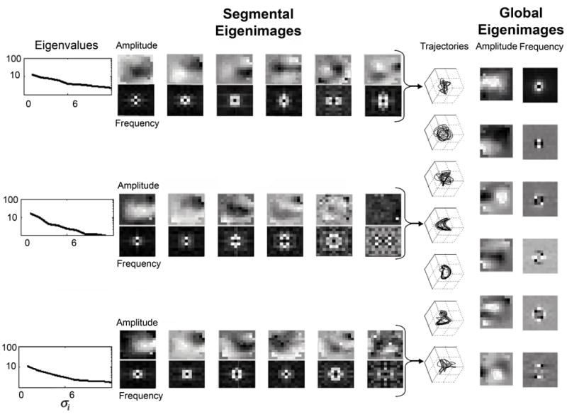
Dynamics from 7 sec oscillatory episode in Fig. 1. At the left side are shown the eigenvalues corresponding to the first 6 spatial eigenmodes v_i based upon the photodetector amplitudes. Below the amplitude eigenmodes are shown the corresponding spatial frequency eigenmodes. These 3 sets of eigenmodes correspond to seconds 1, 4, and 7 from the episode. The column of trajectory plots from each of the 7 sec shows the relationship between the first three temporal modes u_i. Note the simplification of dynamics during seconds 4–6. On the right are global amplitude and spatial frequency eigenmodes calculated from all 7000 images collected. Gray scale proportional to scaled eigenmode amplitudes.

The first 6 spatial eigenmodes v_i for 3 of the 1 sec segments of data, corresponding to the initial and final irregular wave dynamics, and the middle spiral dynamics, are shown in the left half of Fig. 2. The eigenvalues σ_i corresponding to these dominant modes are shown along the left of the figure. Note that during irregular dynamics there is significant structure throughout all 6 of the eigenmodes shown. During the spiral dynamics, the dynamics are concentrated on the first 4–5 modes, with no significant structure evident to visual inspection in the 6^th mode. We perform a spatial Fourier transform on each frame, and repeat this analysis in wave number space. The plots of the comparable eigenmodes based on spatial frequency are shown beneath each amplitude mode. Again, the concentration of dynamics upon the first 5 modes are apparent during spiral dynamics.

The projection of a single image from the spiral dynamics onto the first 3 spatial eigenmodes, weighted by the corresponding eigenvalue, is shown in Fig. 3. A movie of the full sequence of images from these spiral dynamics is archived at [10]. The modal movie emphasizes the crystalline nature of the brain lattice – neurons are fixed in space, and 'wave' activity is a function of the phase relationships of the firing neurons.

Figure 3.

Data from second 4 from Fig. 2 during a rotational spiral. Top panel shows a single spatial image of raw data, while bottom rows show inner product of spatial image on eigenmodes 1, 2, and 3. A movie showing the temporal sequence of these projections is archived at [10].

The spatial eigenmodes v_i are linear combinations of the raw data snapshots f (t, x) , and as such can only reflect the dynamics observed within the sample of data used for the SVD. We can use all of the observed data to construct this basis, and the result of such global SVD analysis are shown in the first 6 amplitude and frequency eigenmodes along the right side of the Fig 2. The waves tend to have more compact spatial frequency representations, reflected in the contrast between these global frequency versus amplitude eigenmodes (such wave number representations also have advantages in image correlation spectroscopy of ensembles of fluorophores [11]).

In analogy with incompressible fluid dynamics, one can quantify the number of modes required to account for 90% of the energy in the signal as

$$E(m)=\frac{{\displaystyle \sum _{i=1}^m}{\lambda }_i^2}{{\displaystyle \sum _{i=1}^n}{\lambda }_i^2},m<n,m=min(m\mid E(m)>0.9)$$

where n are the total number of modes in the decomposition.

Sirovich [12] suggested that E(m) is an effective dimension for a dynamical system. We plot in Fig. 4A the partial sums of all ${\displaystyle \sum _{i=1}^n}{\lambda }_i^2,i=1,\dots ,n$, for each value of n. Whereas for the first second (frames 1500–2500) 7 modes are required to account for 90% of the energy, by the fourth second, only 3 modes are required. The dimensional estimates of such an analysis follow closely the trajectory projections in Fig. 2 – spiral and plane wave dynamics within the middle of these episodes live within a slab of phase space corresponding to an effective 2–3 dimensions. We find that the energy tends to concentrate onto a small number of dominant coherent modes as these episodes organize, and then disseminates onto a larger number of modes prior to termination.

Figure 4.

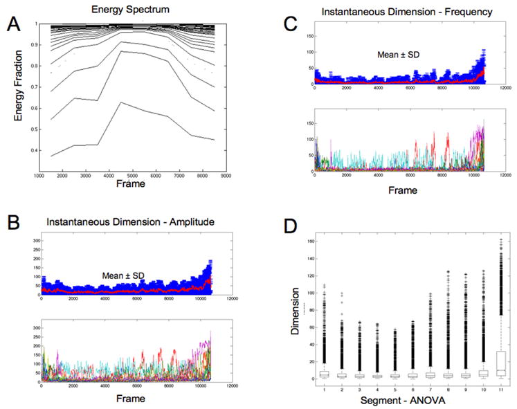
A: Energy fraction plotted for partial sums of modes for example from Figs. 1–3. B: Effective instantaneous dimension d(t)_eff shown for each resampled data set below and as mean and standard deviation above for amplitude, and for spatial frequency in C. D: Box and whisker plot for spatial frequency data shown in C. Each box bounds the 25% and 75% percentiles, and outliers greater than 1.5 times the interquartile range are shown as + signs.

Although the 6 of 13 experiments selected for spiral wave dynamics show a statistically significant reduction in dimension (ANOVA, df=15, F=3.69, p<0.0001) during the spirals analyzed in 1 sec segments (resampled [13] so that all episodes are the same length), we seek a more general description of these dynamics. Instead of recalculating the eigenmodes for 1 sec segments, we employ the global eigenmodes calculated from all of the data (right 2 columns Fig. 2). One can then project each snapshot of the data onto the global eigenmodes, and follow the time sequence of the inner product projections of f(t,x) onto each global v_i , as ${(f,{\mathbf{v}}_i)}^2={\sigma }_i^2{u}_i^2$.

We then create an instantaneous effective dimension, d(t)_eff, by projecting each frame onto the minimum number of sequential eigenmodes required to account for 90% of the instantaneous energy in the signal

$$\begin{array}{l}{(f(t,x),{\mathbf{v}}_i)}^2={\sigma }_i^{2}u{(t)}_i^2,i=1\dots n\\ E{(t)}_m=\frac{{\displaystyle \sum _{i=1}^m}{\sigma }_i^{2}u{(t)}_i^2}{{\displaystyle \sum _{i=1}^n}{\sigma }_i^{2}u{(t)}_i^2},m<n\\ d{(t)}_{\mathrm{eff}}=min\{m\mid E{(t)}_m\ge 0.9\}\end{array}$$

In the plots in Fig. 4B and 4C, the lower plot shows d(t)_eff for individual experiments, while the upper plot shows the ensemble mean and standard deviation at each point in time. For modes composed of voltage amplitude (Fig. 4B), or spatial frequency (Fig. 4C), the dynamics of these phenomena show a monotonic and significant decrease in dimension during the middle of the events (ANOVA: amplitude, F=1950, p<0.00001; frequency, F=2058, p<0.00001), and post-hoc Tukey multiple comparison testing confirms that there is a significant decrease in dimensionality during the middle of these episodes. A box and whisker plot for d(t)_eff calculated from spatial frequency is shown in Fig. 4D (amplitude results are similar). Such simplification, evident when clear spirals and plane waves form, is not at all apparent when more complex patterns are otherwise seen. This analysis demonstrates that the key factor in this dimensional evolution is not the appearance of qualitative spirals or plane waves, but rather depends on more subtle features within the interactions of these neurons.

Our preparation is unusual in that by tangentially cutting a slab of the middle cortical layers, we create as isotropic a piece of mammalian brain as possible, without the masking of activity by superficial cortical layers. Previous optical imaging work analyzing waves from turtle cortex needed to deal with complex signals from the full thickness of the turtle cortex [14]. A recent alternative to optical imaging utilized an array of penetrating electrodes, revealing plane wave structures from a narrow layer beneath the cortical surface carrying motor information in primates [1].

Each of our observed patterns can be composited from the elemental building blocks of the spatial eigenmodes, as seen in projections such as Fig. 3. On the other hand, we recognize that the time sequence of waves such as spirals have a degree of radial symmetry for which SVD may not yield the optimal basis. An alternative radial basis might lead to further simplification of our representation [15], which might have further simplified the characterization of the basic dynamical repertoire of the cortex in these experiments.

There are a variety of events seen in complex nervous systems such as up states [16], spinal cord burst firing [17], and these cortical wavelike events [3], which share the properties that they are episodic, oscillatory, and have apparent refractory periods following which small stimuli can both start and stop such events. We here demonstrate that the wave events have a smooth dynamical evolution where the dimensional complexity decreases and then increases prior to termination. When the dimensionality decreases, the dynamics often exhibit spiral and plane waves.

The biological importance of the dimensional evolution in our findings are likely related to ion shifts into and out of active neurons. We presume that, as shown for intracellular chloride concentration in spinal cord experiments [17], there are one or more order parameters whose temporal course corresponds to the sequence of events shown here. In numerical work, we have shown that using a local mean field model [from Ref. 3], we can demonstrate each of the dynamics described here (irregular, spiral, and plane waves) depending upon the initial conditions (data not shown). Although such basins of attraction exist for such models, without a changing parameter, each pattern would be stable and not evolve in stages as seen here. Since neurons produce a variety of metabolic products, neurotransmitters, and ion shifts as they become more active, there are a variety of candidate parameters available to effect such a sequence of events. On a much larger spatial and far cruder measurement scale, human epileptic seizures also progress through a consistent sequence of dynamical stages [2], and how ion shifts coupled to activity orchestrate such temporal progression remains an open problem.

Nervous systems produce oscillatory patterns on very different scales, whether seizures, motor commands, or wave formation in middle cortical layer slices, which have consistent dynamical evolutions. Further work to define the relevant order parameters that control the evolution of these spatiotemporal dynamics will lead to a better understanding of cortical information processing.

References

- 1.Rubino D, Robbins KA, Hatsopoulos NG. Nat Neurosci. 2006;9:1549. doi: 10.1038/nn1802. [DOI] [PubMed] [Google Scholar]
- 2.Schiff SJ, Sauer T, Kumar R, Weinstein SL. NeuroImage. 2005;28:1043. doi: 10.1016/j.neuroimage.2005.06.059. [DOI] [PMC free article] [PubMed] [Google Scholar]
- 3.Huang X, Troy WC, Yang Q, Ma H, Laing CR, Schiff SJ, Wu JY. J Neurosci. 2004;24:9897. doi: 10.1523/JNEUROSCI.2705-04.2004. [DOI] [PMC free article] [PubMed] [Google Scholar]
- 4.Cross MC, Hohenberg PC. Rev Mod Phys. 1993;65:851. [Google Scholar]
- 5.Stewart GW. SIAM Rev. 1993;35:551. [Google Scholar]
- 6.Sirovich L. Q Appl Math. 1987;45:561. [Google Scholar]
- 7.Holmes P, Lumley JL, Berkooz G. Turbulence, Coherent Structures, Dynamical Systems and Symmetry. Cambridge; Cambridge: 1996. [Google Scholar]
- 8.Senseman DM, Robbins KA. J Neurosci. 1999;19:RC3 . doi: 10.1523/JNEUROSCI.19-10-j0004.1999. [DOI] [PMC free article] [PubMed] [Google Scholar]
- 9.Experimental protocol in accord with the National Institutes of Health Guide for the Care and Use of Laboratory Animals and the Georgetown University Institutional Animal Care and Use Committee.
- 10.See EPAPS Document No. E-PRLTAO-98-082717 for an code and data sample, as well as a movie of modal projections.
- 11.Kolin DL, Ronis D, Wiseman PW. Biophys J. 2006;91:3061. doi: 10.1529/biophysj.106.082768. [DOI] [PMC free article] [PubMed] [Google Scholar]
- 12.Sirovich L. Physica D. 1989;37D:126. [Google Scholar]
- 13.Interpolated resampling performed through a sequence of upsampling, applying an anti-aliasing lowpass finite impulse response filter, followed by downsampling.
- 14.Prechtl JC, Cohen LB, Pesaran B, Mitra PP, Kleinfeld D. Proc Nat Acad Sci. 1997;94:7621. doi: 10.1073/pnas.94.14.7621. [DOI] [PMC free article] [PubMed] [Google Scholar]
- 15.Ruppert-Felsot JE, Praud O, Sharon E, Swinney HL. Physical Review E. 2005;72:016311. doi: 10.1103/PhysRevE.72.016311. [DOI] [PubMed] [Google Scholar]
- 16.Shu Y, Hasenstaub A, McCormick DA. Nature. 2003;423:288. doi: 10.1038/nature01616. [DOI] [PubMed] [Google Scholar]
- 17.Chub N, Mentis GZ, O'Donovan MJ. J Neurophysiol. 2006;95:323. doi: 10.1152/jn.00162.2005. [DOI] [PubMed] [Google Scholar]