Robust Detection of Ocular Dominance Columns in Humans using Hahn Spin Echo BOLD functional MRI at 7 Tesla

Abstract

Cells in the mammalian brain tend to be grouped together according to their afferent and efferent connectivity, as well as their physiological properties. The columnar structures of neocortex are prominent examples of such modular organization, and have been studied extensively in anatomical and physiological experiments in rats, cats and monkeys. The importance of noninvasive study of such structures, in particular in human subjects, cannot be overemphasized. Not surprisingly, therefore, many attempts were made to map cortical columns using functional magnetic resonance imaging (fMRI). Yet, the robustness, repeatability, and generality of the hitherto used fMRI methodologies have been a subject of intensive debate. Using differential mapping in a high magnetic field magnet (7 Tesla), we demonstrate here the ability of Hahn Spin-Echo (HSE) BOLD to map the ocular dominance columns (ODCs) of the human visual cortex reproducibly over several days with a high degree of accuracy, relative to expected spatial patterns from post-mortem data. On the other hand, the conventional Gradient-Echo (GE) blood oxygen level dependent (BOLD) signal in some cases failed to resolve ODCs uniformily across the selected gray matter region, due to the presence of non-specific signals. HSE signals uniformly resolved the ODC patterns, providing a more generalized mapping methodology (i.e. one that does not require experimental parameters or approaches to be adjusted because of potential large vessel effects) that can be – in principle – used to map unknown columnar systems in the human brain, potentially paving the way both for the study of the functional architecture of human sensory cortices, and of brain modules underlying specific cognitive processes.

Introduction

The uniformity of the mammalian cortex has given rise to the proposition that there exist elementary cortical units of operation, consisting of several hundreds or thousands of neurons, that are repeated several times in each cortical area (Lorente de No', 1938). The functional organization of the brain can probably best be understood by analyses at the spatial scale of such units. To understand the organization and operation of microcircuits, one must evidently know a great deal about synapses, neurons, and their interconnections. However, for understanding the functioning of distributed large-scale systems, like those underlying behavior, it is instead necessary to know the nature of the minimal architectural units that organize neural populations of similar properties, and the interconnections of such units.

The cortical columns of neocortex are prominent examples of such structurally and functionally specialized units, and their organization, not surprisingly, has been studied extensively in the early sensory areas of animals ever since their discovery (Hubel and Wiesel, 1959; Mountcastle, 1957). They are clusters of cells with similar properties running perpendicular to the cortical surface, from pia to white matter. In primary visual cortex, such an organization has been demonstrated for preference to the left or the right eye (ocular dominance, OD), contour orientation, direction of motion and spatial frequency (Blasdel and Salama, 1986; Bonhoeffer and Grinvald, 1991; Hubel and Wiesel, 1963, 1977; Shmuel and Grinvald, 1996; Shoham et al., 1997; Weliky et al., 1996). Columnar - or in general tangentially multi-segmented - organization is not a property of primary sensory areas only. Operational modules have been described, for instance, in both early and higher visual association areas, including V2 (Tootell et al., 1983), V4, (Ghose and Ts'o, 1997), V5/MT (Albright et al., 1984), inferior temporal cortex (Fujita et al., 1992), and frontal cortices (Goldman-Rakic and Schwartz, 1982). In addition, a number of cognitive processes are commonly ascribed to cortical subdivisions, a recursive decomposition of which may also require visualization at the micro-architecture level.

It follows, that the development of noninvasive neuroimaging methods that could potentially map the columnar organization of the human neocortex is of paramount importance for both systems and cognitive neuroscience. Of all neuroimaging methods, the one promising sufficient spatial resolution to permit visualization of columnar or laminar subunits is functional magnetic resonance imaging (fMRI) at high magnetic fields (for review and references see (Ugurbil et al., 2003). Hardware advancements and optimization of acquisition techniques in high fields has indeed pushed the spatial resolution of human fMRI from voxel sizes of more than 50 mm³ to less than a single cubic millimeter. The present report demonstrates that the acquisition technique of HSE BOLD in conjunction with high magnetic fields (in this case 7 Tesla) is, in the general case where large vessel effects are not accounted for, ideal for mapping cortical functional architecture.

In the present study, we have concentrated on the ocular dominance architecture of the primary visual cortex as the target of columnar level mapping in humans. In macaque V1, regions of a particular OD are organized in elongated slabs that are locally approximately parallel to each other. The mean cycle along the direction of their shared thinner dimension is 800 μm (Ts'o et al., 1990). Post-mortem studies (Hitchcock and Hickey, 1980; Horton et al., 1990; Horton and Hedley-Whyte, 1984) using cytochrome oxidase staining demonstrated a similar organization in the human visual cortex. The centers of human OD slabs near the V1–V2 border are separated by approximately one millimeter along the thinner slab-dimension (one cycle is approximately 2 mm) and are orthogonal to the border.

In principle, there are several fMRI techniques that could potentially be used for high resolution functional mapping of OD or similar columnar organizations in humans. Arterial spin tagging, which monitors cerebral blood flow, has been shown to be sensitive to the microvasculature and to yield columnar level maps in the cat (Duong et al., 2001); however, it has intrinsically low SNR, especially in human studies. In spite of recent advancements towards high-resolution arterial spin tagging in humans (Pfeuffer et al., 2002a), mapping of sub-millimeter structures in the human brain using this technique is not yet feasible. The use of contrast agents in rats and cats has recently shown promising signs of spatial specificity (Harel et al., 2006; Leite et al., 2002; Lu et al., 2003; Zhao et al., 2005; Zhao et al., 2006). However, the application of such techniques to human studies remains uncertain, because of the dosage requirements as well as the feasibility of doing follow up studies. As a result, currently, the only viable option for high resolution fMRI studies in humans is the blood oxygen level dependent (BOLD) response (Kwong et al., 1992; Ogawa et al., 1992).

One BOLD based fMRI technique employed in animal model experiments (Duong et al., 2000; Grinvald et al., 2000; Kim et al., 2000) exploited the early time points in BOLD contrast (the “initial dip”). First shown in optical imaging studies of intrinsic signals (Frostig et al., 1990; Grinvald et al., 1991; Malonek and Grinvald, 1996), this technique attempts to exploit the early decrease in oxygenation levels for mapping highly localized increases in neural activity within cortical columns. Yet, while detectable with low resolution fMRI in humans (Hu et al., 1997; Menon et al., 1995; Yacoub et al., 1999), this response has proven to be too small in amplitude and too short in duration to yield the contrast-to-noise ratio (CNR) required for high-resolution human fMRI studies. Therefore, columnar mapping in humans using fMRI (Cheng et al., 2001; Dechent and Frahm, 2000; Goodyear and Menon, 2001; Menon et al., 1997) have employed the conventional delayed positive BOLD response (Kwong et al., 1992; Ogawa et al., 1992). One study did attempt to utilize the early portion of the positive BOLD response (Goodyear and Menon, 2001), however, this is also short in duration and difficult to robustly utilize because of the longer total acquisition time (per fMRI volume) required for higher resolution studies.

The positive BOLD response reflects a decrease in deoxyhemoglobin content predominantly due to an increase in CBF that fractionally exceeds the oxygen consumption response generated by altered neural activity (Fox and Raichle, 1986; Hoge et al., 1999). An MRI study conducted using measurement of CBF directly (Duong et al., 2001) has demonstrated that CBF changes can be specific at columnar resolution provided that compulsory and accompanying blood flow increases in large vessels, feeding and draining the activated region, are not simultaneously detected. This was confirmed by a recent optical imaging study (Vanzetta et al., 2004) using CBV measurements as a reflection of CBF; the optical imaging study further demonstrated that maps relying on such CBV, and presumably CBF, changes can be as specific as those obtained by means of the initial dip provided that large surface vessel-signals are nulled. Therefore, the positive BOLD response is also expected to have a component specific to the territory of activated neurons; however, as in CBF or CBV measurements, the BOLD response will also contain inaccurate contributions from large vessels as deoxyhemoglobin changes propagate downstream of the actual site of increased metabolic activity due to blood flow. Therefore, the success of using the positive BOLD effect in high resolution mapping at the columnar level relies on the expectation that non-specific large vessel contributions can be accounted for and thereby either suppressed during data-acquisition or subtracted out from the acquired data.

Gradient echo (GE) or T₂* weighted BOLD imaging of the large positive BOLD response dominates today’s fMRI experiments in humans, including high-resolution studies. This is because of the ease in implementing this technique and its high CNR. This high CNR, however, has been shown to arise primarily from large draining veins, especially at lower magnetic fields (Duyn et al., 1994; Frahm et al., 1994; Kim et al., 1994; Lai et al., 1993; Lee et al., 1995; Menon et al., 1993; Segebarth et al., 1994). Despite this inherent lack of high spatial specificity, previous studies that attempted to map human columns (Cheng et al., 2001; Dechent and Frahm, 2000; Goodyear and Menon, 2001; Menon et al., 1997) have utilized GE BOLD. To overcome the lack of high spatial specificity, these studies employed differential mapping, among other things, to explicitly avoid larger vessels and their effects. With these approaches, non-specific contamination of large vessel signals can often times be diminished, allowing for column mapping. However, the response of these blood vessels might be large in amplitude while extending in space well beyond the vessel location, and variable enough so that differential mapping alone could not completely suppress it, especially if long stimulation durations are employed (Goodyear and Menon, 2001).

Other approaches have been implemented to discern contributions from large vessels in GE BOLD images, for example, bipolar gradients (Boxerman et al., 1995; Song et al., 1996), masking of voxels demonstrating high-amplitude responses (Cheng et al., 2001; Kim et al., 1994; Shmuel et al., 2007), and phase specific information (Menon, 2002). These techniques, however, can result in loss of the activation-specific signals in voxels where large vessel and activation specific signals co-exist, restricting the ability to discern specific signals only to those regions unaffected by large vessels. In this case, inability to detect columnar organizations in parts of the cortex cannot be used as evidence of their absence. Even when column like organizations are detected, unexpected interruptions of such organizations due to less than ideal imaging techniques can lead to questions about the validity of the measurement unless there exists a priori knowledge about the existence of such columnar organizations. For example, in previous work on imaging OD columns (ODCs) with fMRI, columns were not detected in some regions of V1 due to short comings of the technique. However, because of a priori knowledge (Horton and Hedley-Whyte, 1984), it is realized that the technique fails in some parts of the cortex but not in others. For the purposes of this work, it is assumed that success or accuracy in mapping ODCs can be assessed by the resemblance of the functional maps to the post-mortem human data (Hitchcock and Hickey, 1980; Horton et al., 1990; Horton and Hedley-Whyte, 1984).

It has been more than 5 years since the last report of columnar organization in humans despite the continuous increase in the number of MRI systems in addition to the number of high field MRI systems. The primary reason for this is presumably because of the problems mentioned above which make it extremely difficult to generalize the methods and techniques of the previous human studies to other functional systems and cortical areas. Furthermore, the vast majority of all fMRI studies employ GE BOLD at low fields. While there is a general push to higher magnetic fields (currently 7 Tesla), there is virtually no push to use an alternative contrast because there has been no qualitative evidence of any advantage over GE BOLD. High field BOLD imaging alleviates the problems discussed above, and does undoubtedly enhance tissue signals (Yacoub et al., 2001), as well as provide higher SNR, which is a prerequisite for images of high spatial resolution. In our recent studies (Yacoub et al., 2003; Yacoub et al., 2001; Yacoub et al., 2005) we have indeed demonstrated highly sensitive and spatially specific GE and Hahn Spin Echo HSE BOLD images at high fields. However, superior spatial specificity can be accomplished by the implementation of HSE BOLD imaging at high fields (Goense and Logothetis, 2006; Harel et al., 2006; Lee et al., 1999; Lee et al., 2002; Yacoub et al., 2003; Yacoub et al., 2005; Zhao et al., 2005; Zhao et al., 2006; Zhao et al., 2004). This is true because, compared to GE BOLD, HSE BOLD at high (but not low) fields is substantially less sensitive to large vessel signals (Harel et al., 2006; Yacoub et al., 2005; Zhao et al., 2006; Zhao et al., 2004), and its CNR at high fields such as 7 Tesla, is sufficient to generate reliable responses at sub-millimeter spatial resolutions.

In the present study, we demonstrate the power of the HSE BOLD technique by using it to robustly and reliably map columns in human visual cortex. Our findings demonstrate for the first time that the highly spatially specific HSE fMRI technique applied at 7 T, can be employed to map the cortical micro-architecture of the human cortex without the necessity of constraints based on a priori knowledge of the vascular anatomy or time course of BOLD signal responses. In addition, GE fMRI succeeds only if large vessel signals can be accounted for and/or do not contaminate the gray matter region of interest. Thus, establishing the HSE technique as a more reliable mapping tool which in turn may open new avenues of research to map unexplored functional systems in the human brain.

Methods

Subjects

Three healthy subjects (males, ages: 19–26) participated in this study after providing informed written consent to the experimental protocol. The human subjects’ protocol was approved by the institutional review board at the University of Minnesota. Subjects were pre-screened during pilot studies, according to their ability to use a bite bar and remain still during long sessions.

Visual stimulation

Visual stimuli were delivered by means of fiber optics (Silent vision, Avotec Inc., Stuart, FL), providing visual fields of 23º × 30º. For obtaining a clear focused image and maximum field of view, subjects were instructed to adjust the position and focus at the beginning of each session by themselves. The Avotec eye pieces were then mechanically fixed to the radiofrequency (RF) coil holder. Subjects were instructed to fixate on a fixation spot throughout the entire scan, during both stimulation and control periods. To maximize the imaged responding cortical area, the fixation spot was presented 5º away from the center, either in the upper (for lower visual field stimulation) or the lower (for upper visual field stimulation) part of the image. The lower or upper visual field was stimulated according to which bank of the calcarine fissure was imaged, upper or lower bank, respectively. Each scan started with a control period of 48 s in which a blank gray image was presented binocularly. This control period was followed by 8 epochs of 48 s monocular stimulation each, alternating between stimulation of the left and the right eye with high-contrast radial checkers flickering at 8 Hz. The checkers were presented to the stimulated eye, while a blank gray image, identical to that presented during the control period and with luminance equal to the mean luminance of the checkers, was presented to the non-stimulated eye.

Hardware for functional MRI

fMRI was conducted on a 7 T whole body system with a 90 cm bore, driven by a Varian (Palo Alto, CA) INOVA console running VNMR. The system was equipped with a MAGNEX (Oxford, U.K.) head gradient set, which was torque-balanced, self-shielded, and water-cooled (inner diameter: 38 cm). The gradient coil was driven by a Siemens gradient amplifier capable of 800V/400A. The gradient setup could achieve a maximum gradient of 4 Gauss/cm in 200 μs. To maximize sensitivity in the visual cortex while maintaining uniform spin refocusing for HSE acquisitions, a half volume radio-frequency (RF) coil was used for transmission, and a small (6 cm ) quadrature coil was used for reception (Adriany et al., 2001). These coils were actively detuned during acquisition, via TTL signals sent by the imaging sequence at the appropriate times.

Functional MRI data acquisition

Each subject was scanned on six different days: 3 sessions were devoted to GE BOLD imaging, while the 3 other sessions were devoted to HSE BOLD imaging. For GE imaging, we relied on the methods that were previously used for high-resolution imaging (Cheng et al., 2001; Menon et al., 1997). Previous studies that utilized GE BOLD imaging to successfully demonstrate columnar patterns in humans (Cheng et al., 2001; Menon et al., 1997) used extensive image segmentation. For the purpose of this work we assumed this approach to be acceptable for high-resolution GE BOLD images. Thus, for GE imaging we applied a 12 segment Echo-Planar Imaging (EPI) sequence with a full field of view (FOV) (9.6 x 12.8 cm²) and a 192 x 256 matrix size. The image TR/TE was 6 s / 25 ms and the total readout time was 25.6 ms (1.6 ms / line).

For HSE imaging, we have previously demonstrated (Duong et al., 2002; Yacoub et al., 2003; Yang et al., 1997) that taking advantage of the 180 degree pulse, and using a reduced (slab-selective) FOV acquisition, high resolution images can be acquired in a few segments, thereby allowing for maximal acquisition efficiency. For HSE imaging, 4 segments were used with a reduced FOV (3.0 x 12.8 cm²) and a 60 x 256 matrix size. The image TR/TE was 6 s / 55 ms and the total readout time was 24.0 ms (1.6 ms /line). For both types of data acquisition the nominal in plane spatial resolution was 0.5 × 0.5 mm². However, the spatial resolution along the phase encoding direction could be expected to be blurred because of the T₂* filter effect during the EPI readout. In our case, the effective spatial resolution in the tissue, determined by the full width at half maximum of the point spread function of the T₂* filter effect, was only slightly (4%) larger than the nominal spatial resolution because the readout time for one segment was approximately equal to the T₂* of the tissue (Haacke et al., 1999). For optimizing magnetic field homogeneity, automatic shimming methods based on multiple axis field mapping (Gruetter and Tkac, 2000) were implemented, facilitating fast and localized shimming.

Selection of the imaged slice

For both GE and HSE we imaged a single 3.0 mm thick slice. A flat, minimally curved gray matter area, as posterior as possible within the upper or lower bank of the calcarine fissure was considered optimal (Cheng et al., 2001). Imaging a flat region within one of the banks of the calcarine sulcus maximizes the area with predictable geometry of human ODCs (Cheng et al., 2001; Horton et al., 1990), and therefore facilitates the evaluation of the acquired data. In addition, the signal drops rapidly as a function of distance from the plane of the small surface receive coil. Thus, imaging a region as close as possible to the skull allows for maximum sensitivity to functional signals. The target region selection was based on multiple sagittal T₁ weighted scout images acquired in pilot scans for each subject. Fig. 1 shows two of these sagittal images from one subject. The geometry of the calcarine sulcus is not necessarily symmetric for the two hemispheres. Both the right hemisphere and left hemisphere were assessed according to the criteria mentioned above. One hemisphere was selected, while the other was discarded (Fig. 1). Ultimately, the slice was positioned parallel to – and overlapping with - a relatively flat gray matter region. We did not explicitly make attempts to avoid any nearby or neighboring vessels as was done previously (Cheng et al., 2001). This flat gray matter region was then subsequently used in analyzing the data. Subject positioning and slice selection was kept as similar as possible during all 6 sessions of each of the subjects. Fig. 2 depicts an example of the slice matching in one subject. It shows the imaged slices used in 3 different days from the same subject.

Figure 1.

An example of slice selection from subject 3. The slice was optimized for covering the flat portion of cortex within the lower bank of the calcarine fissure in the right hemisphere (RH). The ODCs from the right hemisphere are expected to run within the slice orthogonally to the midline.

Figure 2.

An example of matching slices obtained on different days from subject 3. The 3 images depict the imaging slice selected from the same subject on 3 different days. The images from day 2 and 3 were registered to the image from day 1 (the image to the left). The red arrows point to the same landmarks as they appear on the 3 different images. The green box indicates the flat gray matter region within the calcarine fissure that was selected as the ROI.

Minimizing and handling head movements

Each of the subjects used a bite bar made to match the subject’s dental impressions using hydroplastic material (Tak systems, Wareham, MA). The bite bar was attached to a bar, which in turn was bolted to the RF coil holder.

Since we imaged only one slice, we could off-line apply head motion detection and correction that caused translation and rotation of the image within the imaged plane. We could not, however, use the same strategy to detect motion along the axis orthogonal to the imaged plane. To control for this type of movement, we monitored the slice position during each session. Prior to the beginning of an fMRI session, seven T₁ weighted adjacent sagittal images were taken from the mid-line towards the selected hemisphere. During the session, after each fMRI scan, we repeated this procedure and compared the position of the slice used for the functional scan to its position before a given fMRI scan had begun. (i.e. we checked whether significant accumulative subject motion could be observed). In the event of subject movement, the slice was repositioned to match the slice position during the previous scans.

The ~7 min. fMRI runs were repeated as tolerated by the subject. In an average session, the subject was able to participate in 8 –10 scans. The subjects were in the scanner for approximately 2 – 2.5 hours.

Each of the data sets from a single session was analyzed for subject motion that caused translation and/or rotation of the image within the imaged plane. We analyzed head movement both within – and between scans of each session. Data from scans in which significant motion (mean absolute deviation from the mean position for that day > 250 μm) was detected relative to the rest of the data from the session were discarded from the final analysis. Data from approximately 1–2 scans per session were discarded due to mis-registration or motion of the subject. The average motion parameters for the scans which were used in the averaging were: translation: 0.14 mm ± 0.04 mm and rotation: 0.38º ± 0.15º (mean ± SD of absolute deviation for both parameters).

Data Pre-processing

The raw fMRI data were pre-processed with a rapid correction scheme (Pfeuffer et al., 2002b) to reduce respiration induced B₀ fluctuations. The corrected k-space data were then zero filled and reconstructed to yield images with in plane voxel sizes of 0.25 mm. Motion correction followed, using AIR (Woods et al., 1992) to correct for motion within – and between – scans as described above. Scans from the same session were averaged together provided the mis-registration between them (before motion correction) was not significant.

Alignment of fMRI images obtained in different days

To assess reproducibility of the maps across different sessions, the data from each subject obtained in different days were registered to each other using an automated algorithm. Registration between days was done separately for GE and HSE data. We first computed the mean image per session, averaged across the data obtained from one day. Next, parts of the mean image with low sensitivity (low acquired image signal) were discarded. All of these regions were outside of the region of interest (ROI), in regions that were distant from the receive coil. In addition, the effort we made to position the subject and slice identically across all sessions was in most cases successful in the target region and its close proximity. However, occasionally, regions outside the ROI were observed to be dissimilar across the 3 different days. These regions were discarded as well.

In summary, for the registration between sessions, we used the ROI and regions in proximity to it with high sensitivity that encompassed the same anatomical regions and with an image pattern that was similar across the 3 different sessions. The 3 trimmed mean images constituted stable data that could be used for registration across days. Registration was performed using the Flirt tool, part of the FSL fMRI analysis software (Jenkinson et al., 2002; Smith, 2004). Registration was performed using translation and rotation in plane, by maximizing the normalized correlation between the images. The trimmed image from one day was used as a reference for registering the images from the two other days. These two registrations yielded 2 transformation matrices that were applied to register the data from the corresponding 2 days. The transformation corresponding to a registered session was applied to each of the images acquired during the session. To allow sub-voxel resolution of the registration process, sinc interpolation was used.

Statistical maps

Statistical maps and the following quantitative analysis were done in Stimulate (Strupp, 1996), PV-WAVE (Visual Numerics, Houston, TX), and self written routines in MATLAB (the MathWorks, Naticj, MA). Voxel-wise t-test analysis was applied to test whether the response was higher during epochs of left or right eye stimulation. The same statistical threshold was used for all studies (GE and HSE) (p < .15, for differential significance (R-L), and p<0.01 for (R-D) or (L-D)). fMRI maps indicate in a binary manner (red or blue, for right or left eye, respectively) those voxels which passed both differential (R-L) and either (R-D) or (L-D) statistical significance.

Reproducibility

To qualitatively assess the reproducibility of the data, ODCs were marked with arrows according to the overlap HSE fMRI maps from the different days. The pattern of these arrows was then projected onto the registered data of the same subject from the different days (Fig. 3–5). The same set of arrows was superimposed onto the registered GE maps corresponding to the approximate locations that were determined according to anatomical landmarks and the GE overlap map.

Figure 3.

Differential functional OD maps depicting increased activity for left eye stimulation (blue) and right eye stimulation (red) for Subject 1. The upper and lower rows depict the maps obtained using GE and HSE fMRI, respectively. (A–C) OD maps from 3 different GE sessions. These maps were obtained after registering the functional data from day 2 (B) and day 3 (C) to the data from day 1 (A). (D–E) The overlap between maps obtained in the 2 most reproducible GE sessions (D) and all 3 (E) of these GE sessions. For computing the maps presented in D–E, the differential maps obtained in different sessions were spatially filtered (see methods). A logical AND operator was applied to the maps obtained on different days. In D, the maps obtained in days 1 and 3 (presented in A and C) are compared. Red or blue colored voxels passed the threshold on the 2 (D) or all 3 (E) days, and showed consistent eye preference over days. The bottom row depicts in an identical format the maps obtained from 3 different HSE sessions with registered data (F–H), and the overlap between maps obtained in 2 (I) and all 3 (J) HSE sessions. In I, the maps obtained in days 1 and 2 (presented in F and G) are compared. The registrations of GE data (A–E) and HSE data (F–J) were performed separately. The superimposed arrows were positioned according to the HSE overlap map shown in (I), and copied to locations that are identical relative to the registered HSE data (F–J). Therefore they can facilitate the evaluation of reproducibility. The same set of arrows was superimposed onto the registered GE maps corresponding to the approximate locations that were determined according to anatomical landmarks and the GE overlap map shown in (D). The same statistical threshold was used for all studies (p < .15). The background image in A–C and F–H are the BOLD GE and HSE images, respectively. The background gray level images in D–E and I–J show the differential OD response averaged over the compared 2 or 3 sessions. Pos, posterior; RH, right hemisphere, IHF, Inter-hemispheric fissure.

Figure 5.

Differential OD maps obtained from Subject 3. The upper and lower rows depict the maps obtained using GE and HSE fMRI, respectively. The analysis procedure and format of presentation are identical to those used in Fig. 3. In D, the maps obtained in days 1 and 2 (presented in A and B) are compared. In I, the maps obtained in days 1 and 2 (presented in F and G) are compared.

Furthermore, to quantitatively assess the reproducibility of the OD map across different days, a voxel by voxel comparison was performed. We computed the fraction of voxels that passed the statistical threshold consistently on two imaging days (i.e., we applied a logical operator of (Leye and Leye) or (Reye and Reye)). In addition, the voxel-wise t-values from a given day were plotted against t-values from the other days. The correlation coefficient, the slope derived from orthogonal fitting, and the corresponding p-values were calculated. Prior to the voxel-wise quantification of reproducibility, spatial filtering was applied to the differential ODC maps. We applied a circularly symmetric band-pass filter that filtered out frequencies with cycles shorter than 1 mm and longer than 12 mm. The isotropy of the filter ensured that it could not induce artifactual anisotropic maps.

Comparison of GE and HSE differential responses

A t-statistic analysis was computed separately for the data from each session and subject, as described above. The same statistical threshold was used across different sessions and type of imaged signal (HSE or GE BOLD). To quantify the contrast between the responses to stimulation of each of the eyes, fMRI time courses were sampled from individual activated voxels. The time courses we considered were averaged only over regions where right or left eye ODCs were identified in both GE and HSE differential activation maps. To compare the responses of GE and HSE signals as directly as possible, the regions of interest used to sample the time courses from GE and HSE imaging sessions were matched according to anatomical features within the imaged slice (within a given image contrast they were approximately identical, because the data within an image contrast were registered across days). Response amplitudes were defined as the mean percent change from baseline (baseline data was acquired at the beginning of each scan) for a given eye over all the stimulation periods for that given eye. Subsequently this contrast was compared between GE and HSE data from the same subject.

Spatial analysis of ocular dominance maps

The mean width of the columns and the corresponding length of a cycle were quantified by applying a Fourier Transform to the differential functional map within the predefined ROI. The principal spatial frequency of the organization, its power relative to that of frequencies in the center of the frequency domain and the direction of its anisotropy were identified. These parameters were determined according to the center of a region in the frequency domain that demonstrated the maximum increased power, and did not correspond to the zero frequency.

Assessment of false positives

To asses the level of false positives in this high field HSE mapping technique, one of the subjects was scanned in two additional sessions. During these additional sessions, the stimulation paradigm was identical to that used during the other 6 sessions, except for using binocular instead of monocular stimulation. The HSE BOLD technique was used with the same imaging parameters and slice as in the monocular studies. The analysis procedure we applied and the two regressors we used were identical to those applied to the data obtained with monocular stimulation.

Results

Results from three subjects are shown in Figs. 3–5, respectively. Fig. 3 shows ODCs obtained from subject 1, with panels A–C displaying the pattern of columns obtained using GE BOLD from 3 different days, respectively. To demonstrate these patterns, the data from the 3 different days were spatially registered. The yellow and cyan arrows mark identical locations on all GE maps (Fig. 3 A–E). The region of the imaged flat cortex within the calcarine sulcus is zoomed. The vertically running dark elongated region in the background is the inter-hemispheric fissure. Alternating elongated strips with preference for left and right eye run approximately perpendicular to the inter-hemispheric fissure. The pattern of these strips is clearer within the more anterior region. Fig. 3D depicts the voxel-wise overlap (logical (L AND L) OR (R AND R) operator) between the patterns of OD obtained in two of the GE sessions. Fig. 3E depicts the overlap between the patterns obtained in all 3 GE days (similar operator applied to all 3 days). Prior to the application of the logical operator, the maps from individual days were band-pass filtered (see methods). Qualitatively, the pattern obtained for the OD map was reproducible across the 3 different GE days of data acquisition. Note that the less ‘column like’ part of the map, within the posterior part of the image was largely reproducible as well.

Fig. 3F–H depicts the pattern of columns obtained using HSE BOLD from 3 different days from the same subject and region. The HSE data from the 3 different days were spatially aligned. The alternating elongated strips with preference for left or right eye were also detected with the HSE BOLD signal. The organization detected with the HSE signal is finer than that obtained with the GE signal. The anterior part shows a clearer ‘column like’ pattern, as expected from post-mortem data, in the HSE maps compared to the GE maps, and this pattern continues into the posterior regions of the slice in the HSE maps (especially in Fig. 3G–H) but not in the GE maps. Fig. 3I–J depicts the voxel-wise overlap between the patterns obtained using HSE imaging, in a format identical to that of Fig. 3D–E. The features of reproducibility seem similar when comparing GE to HSE data obtained from subject 1. The fine pattern of ODCs obtained using the HSE signal was largely reproducible across 3 days.

Analogous results from subject 2 and 3 are presented in Fig. 4 and Fig. 5, respectively, in a format identical to that of Fig. 3. In subject 2, the HSE data demonstrate clear strips of differential preference for the left or the right eye (Fig. 4F–H). These strips are elongated and run approximately perpendicular to the inter-hemispheric fissure. Moreover, they show considerable reproducibility across the 3 days of data acquisition (Fig. 4I–J). While the GE data demonstrate reproducibility (Fig. 4D–E), these data lack any apparent ODC like patterns (Fig. 4A–C). Instead, the GE data is dominated by 2–4 mm wide regions with preference to one eye or the other. Results from subject #3 are shown in Fig. 5. The HSE data demonstrate a fine ODC like pattern (Fig. 5F–H), with considerable overlap across the 3 days of data acquisition (Fig. 5I–J). In contrast, the GE data depict these columns only in the anterior portion of the region and do not appear to be successful in resolving the columns in the posterior regions. Overall, as is the case for each of the 3 subjects, reproducibility across 3 different days was demonstrated in the series of GE and HSE sessions, respectively. The spatial reproducibility of the differential maps was observed irrespective of whether it resolved an OD like pattern or not. In the imaged flat gray matter regions, HSE BOLD imaging resolved an extremely predictable OD like pattern; while only in some of these regions did GE BOLD imaging resolve such a pattern.

Figure 4.

Differential OD maps obtained from Subject 2. The upper and lower rows depict the maps obtained using GE and HSE fMRI, respectively. The analysis procedure and the format of presentation are identical to those used in Fig. 3. In D, the maps obtained in days 1 and 3 (presented in A and C) are compared. In I, the maps obtained in days 1 and 2 (presented in F and G) are compared.

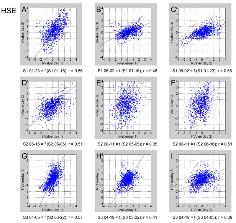
To quantify the spatial reproducibility of the demonstrated OD maps, we examined their day-today reproducibility. Fig. 6 demonstrates the reproducibility obtained using GE signals. Fig. 6A shows the scatter plot of the voxel-wise differential t-values obtained in day 2 plotted against the corresponding t-values obtained in day 1 from subject 1. Similar scatter plots show the data from the same subject obtained in day 3 against day 1 (Fig. 6B) and day 3 against day 2 (Fig. 6C). Significant correlation was obtained for all 3 comparisons (r = 0.62, 0.74 and 0.51 for A, B, and C respectively; see Table I D–I for p-values and regression slopes). Fig. 6D–F demonstrates the day-to-day reproducibility of the OD maps obtained from subject 2 using GE signals. Although a smaller proportion of the variance can be explained by reproducible differential OD signal here (r = 0.49, 0.51, and 0.42), the maps were significantly reproducible over sessions (Table I). The bottom row shows the scatter plots obtained from subject 3, with clear reproducibility of the GE differential OD maps. Overall, although the GE signals did not demonstrate a fine OD pattern as the HSE signals did, they were nonetheless still reproducible.

Figure 6.

Reproducibility across days of ODC maps obtained using GE BOLD signals. Plots show the scatter of t-values of individual voxels from one scan day versus the t-values of the corresponding voxels from a second scan day. The data from each pair of compared days were spatially aligned. The first, second, and third row presents comparisons of imaging sessions of subject 1, 2, and 3, respectively. All voxels which passed the differential statistical threshold, irrespective of any column-like patterns were used in the analysis. Voxels that fall in the upper right quadrant demonstrated preference for right eye stimulation on both days. Voxels in the lower left quadrant demonstrated preference for left eye stimulation on both days. The preference for eye stimulation of voxels in the other quadrants was not reproducible over the 2 sessions. The straight line depicts regression using orthogonal fitting.

Table I.

Reproducibility of ocular dominance maps obtained from different sessions.

a) Subject and method	b) % overlap day 1 and day 2	c) % overlap all 3 days	d) Slope of regress.: day 1 and day 2	e) correlation coefficient and p-value, day 1 and day 2	f) Slope of regress.: day 1 and day 3	g) correlation coefficient and p-value, day 1 and day 3	h) Slope of regress.: day 2 and day 3	i) correlation coefficient and p-value, day 2 and day 3
s1 GE	87.60	65.56	1.11	0.62 1.17e–143	0.88	0.74 8.79e–231	0.74	0.51 3.45e–091
s2 GE	70.56	46.47	2.71	0.49 5.04e–077	1.57	0.51 1.23e–084	0.50	0.42 1.72e–053
S3 GE	86.99	68.32	1.34	0.64 8.82e–188	1.14	0.60 2.70e–157	0.80	0.47 6.57e–091
S1 HSE	78.52	59.08	1.33	0.56 6.08e–111	0.41	0.48 8.48e–077	0.36	0.55 4.26e–108
S2 HSE	58.73	43.34	0.86	0.51 7.89e–084	2.61	0.35 5.48e–037	2.29	0.51 4.05e–084
S3 HSE	80.98	50.44	1.91	0.57 1.53e–142	1.41	0.41 3.56e–065	0.46	0.29 7.56e–033
GE mean±SD	81.8±9.6	60.1±11.9	1.72±0.86	0.58±0.08	1.19±0.34	0.62±0.12	0.68±0.15	0.47±0.05
HSE mean±SD	72.8±12.2	51.0±7.9	1.37±0.56	0.54±0.03	1.48±1.10	0.41±0.06	1.04±1.09	0.45±0.14

In b), the number of voxels that passed the threshold consistently on both days divided by the number of voxels that passed the threshold on both days. The expected value based on the null hypothesis (voxel-wise preferred eye is random) is 50%. In c), a similar measure as in b), applied to all 3 days. The expected value based on hypothesizing random voxel-wise preferred eye is 25%. In d), f), and h), slope of regression using orthogonal fitting of voxel-wise t-values. In e), g), and i), correlation coefficient between voxel-wise t-values, and p-value of testing whether the computed correlation could be sampled from two uncorrelated populations. The measures here are for the ODC maps that were spatially filtered (see methods).

Fig. 7 demonstrates the reproducibility of OD maps obtained using HSE signals, in a format identical to that of Fig. 6. For each of the 3 subjects and each of the 3 possible pairs of days, significant reproducibility was obtained. Interestingly, the reproducibility measures obtained from subject 2 using GE signals (with patterns that did not resolve ODCs) were lower than those obtained using HSE signals. Table I summarizes the reproducibility measures obtained using GE and HSE signals from all 3 subjects. The average fraction of all voxels that showed consistent OD preference over two scan days using GE was 81.8±9.6%, while the corresponding fraction using HSE was 72.8±12.2% (compared to 50% consistency if the preference was random). The average fraction of voxels that showed consistent preference over all three scan days using GE was 60.1±11.9%, while the corresponding fraction using HSE was 51.0±7.9% (compared to 25% consistency if the preference was random). The voxel-wise t-values obtained from each pair of days were correlated. Overall, the maps obtained using both types of signals were reproducible over days in a statistically significant manner. On average, the reproducibility measures obtained using GE signals were higher than those obtained using HSE signals when the entire gray matter area was analyzed, irrespective of columnar organization.

Figure 7.

Reproducibility across days of ODC maps obtained using HSE BOLD signals. The format of presentation is identical to that in Figure 6.

To control for false positive detection, we ran 2 additional HSE imaging sessions, in which instead of using alternating monocular stimulation (each eye at a time), we used binocular stimulation. Otherwise, the experimental paradigm and analysis procedure were identical to those used for monocular stimulation. Fig. 8A and B show the results obtained from subject 2 from two different days. The superimposed arrows depict the locations indicated on the maps obtained from the same subject using monocular stimulation (Fig. 4F–H). In contrast to the pattern of OD seen in this subject using HSE and monocular stimulation, no similar pattern could be detected using binocular stimulation. In the absence of instrumental and physiological noise, the differential analysis (both eyes relative to both eyes) applied to these data should result in a flat map (no difference). Some regions did show differential activity above the threshold. However, the lack of coherent organization suggests that the regions which showed differential preference were the expected result of multiple statistical comparisons (i.e. false positives). Consistent with that notion, the fraction of differential activity that was reproducible across the 2 days was null (0%; Fig. 8C), and the corresponding scatter plot of t-value reproducibility did not show a trend of linearity (Fig. 8D). Similarly, no reproducibility was detected when plotting the t-values from each of these binocular stimulation sessions against the t-values obtained from a monocular stimulation session (Fig. 8E–F). We therefore concluded that the OD maps (Figs. 3–5) we obtained could not be the result of false positive detection.

Figure 8.

Estimation of false positive ODC detection: functional maps depicting differential analysis of HSE data obtained during binocular stimulation. (A) and (B) depict the results of 2 different sessions from subject 2. The data were registered to the HSE data presented in Fig. 4. The arrows were copied from Fig. 4 and registered to the same anatomical landmarks. The activated voxels here are a measure of false positive detection resulting from the data acquisition and analysis procedures we used. (C) The overlap between maps presented in (A) and (B). The differential maps obtained in different sessions were spatially filtered (see methods). A logical AND operator was applied to the maps obtained on different days, in a manner similar to that used for the reproducibility map presented in Fig. 4I. (D) Reproducibility across days of the differential t-values computed using differential analysis of HSE data obtained during binocular stimulation. The data used for the map shown in B is presented as a function of the data used for the map in A. The data from the two compared sessions were spatially registered prior to the analysis. The format of presentation is identical to that in Figs. 6–7. In contrast to the reproducibility shown in Fig. 7, the scatter plot shows a random relationship here. (E) The data used for the map shown in A (with binocular stimulation) is presented as a function of the data used for the map in Fig. 4F (with monocular stimulation). (F) The data used for the map shown in B (with binocular stimulation) is presented as a function of the data used for the map in Fig. 4F (with monocular stimulation).

Even though the GE maps in the high magnetic field used in this study were highly reproducible (even more so than HSE maps), they did not always resolve ODC like patterns (Figs. 3–5). To quantify this phenomenon, we computed the 2D spatial frequency (Fourier power) of the differential maps obtained in the selected flat portion of the gray matter parallel to the calcarine sulcus from each of the subjects. The top row of Fig. 9 shows HSE data averaged for each subject. Increases in power can be seen for frequencies of ~ 0.5 cycles/mm. The peaks are located above and below the center, indicating that the increase in this frequency is approximately parallel to the inter-hemispheric fissure, consistent with the pattern of elongated ocular preference strips that run orthogonal to this fissure (Figs. 3–5). Based on this increase in power, the mean width of ODCs from HSE BOLD imaging was 1.06 ± 0.10 mm (Table II). The bottom row presents the results from GE studies. Increases in power that approximately corresponded to the frequencies detected with HSE imaging were observed in subjects 1 and 3 (mean width 1.16 ± 0.09 mm). For both subjects, the power around these peaks relative to the power in the center of the frequency space was higher in the HSE data than in the GE data (Table II), indicating that the organization obtained using GE imaging was not as clear as that from HSE imaging. Consistent with the lack of ODC patterns in the GE data of subject 2 (Fig. 4), no corresponding increase in power was observed in that data. The increase in power associated with frequencies and orientation expected from ODC maps justifies the use of the band-pass filter we employed prior to estimating the reproducibility (Figs. 3–5).

Figure 9.

Spatial frequency distribution of the differential OD maps. Each of the presented distributions is the average over the 3 spatial frequency distributions obtained in 3 sessions from one subject. HSE BOLD and GE BOLD maps are shown at the top and bottom row, respectively. The data from Subject 1 (left) showed clear peaks approximately at the expected orientation (above and below the center, representing the anterior-posterior axis) and spatial frequency (0.5 cycles / mm) of OD maps, for both GE and HSE data. The data from Subject 2 (center) showed clear peaks at the expected locations for the HSE BOLD data. In contrast, no increased power was observed in those locations for the GE data. The data from subject 3 showed a clearer increase in power at the expected locations for the HSE data than for the GE data. The arrows indicate the locations of the observed increase in power in frequencies approximately expected for ODCs (~ 0.5 cycles / mm, oscillating along the anterior-posterior axis).

Table II.

Mean width and relative power of ocular dominance columns.

a) Subject and measure	b) GE Day 1	c) GE Day 2	d) GE Day 3	e) GE mean±SD	f) HSE Day 1	g) HSE Day 2	h) HSE Day 3	i) HSE mean±SD
S1, width	1.11	1.06	1.08	1.08 ±0.025	1.06	1.09	0.85	1.00 ±0.13
S1, power	0.81	0.57	0.54	0.64 ±0.15	0.6	1.03	1.96	1.20 ±0.70
S2, width	N/A	N/A	N/A	N/A	0.92	0.96	1.12	1.00 ±0.11
S2, power	N/A	N/A	N/A	N/A	1.18	1.1	1.17	1.15 ±0.04
S3, width	1.28	1.20	1.21	1.23 ±0.04	1.20	1.23	1.08	1.17 ±0.08
S3, power	0.36	0.33	0.39	0.36 ±0.03	1.11	2.6	1.04	1.58 ±0.88
Width mean±SD	1.16±0.086				1.06±0.098
Power mean±SD	0.50±0.18				1.31±0.60

Ocular dominance columns widths (in mm) from 3 subjects scanned on 6 different days (3 HSE and 3 GE). The widths were determined from the spatial frequency of the ODC maps (as shown in Figure 9). The relative power was calculated by dividing the mean power averaged within a radius of 0.1 cycle/mm around the peak of the ODC map frequency by the mean power averaged within a similar radius around the center of the frequency space.

The finer pattern of OD resolved by HSE signals (Figs. 3–5, 9) in part arises from the higher differential contrast of HSE signals compared to GE signals. Fig. 10 shows the mean contrast between the 2 eyes for the 2 subjects from which ODCs were obtained using both GE and HSE imaging (subjects 1 and 3). The bars to the left depict the response relative to baseline. The response relative to baseline within the ODCs with preference to the stimulated eye was consistently higher in the GE data (5.88 ± 0.90 % (subject 1), 2.71 ± 0.36 % (subject 3)) than in the HSE data (3.70 ± 0.95 % (subject 1), 1.87 ± 0.37 % (subject 3)). However, the differential contrast between the ODCs showing preference to the stimulated eye and the non-stimulated eye was higher in the HSE data (1.82 ± 0.23 % (subject 1) and 1.01 ± 0.41 % (subject 3)) than in the GE data (0.86 ± 1.10 % (subject 1) and (0.88 ± 0.46 % (subject 3)). To quantify the differential contrast relative to the global response from baseline we computed a selectivity index ((% change in ODCs representing the stimulated eye - % change in ODCs representing the non-stimulated eye)/ % change in ODCs representing the stimulated eye). The mean selectivity index averaged over voxels, sessions, and the two subjects was 0.52 ± 0.005 for HSE data and 0.24 ± 0.13 for GE data. Overall, while the global response relative to baseline was higher in the GE data, both the selective response and the selective response relative to the global response were higher in the HSE data.

Figure 10.

BOLD response relative to baseline from subject 1 and subject 3, respectively, for GE and HSE data from ODCs showing preference to the stimulated (labeled ‘STIMULATED’) and the non-stimulated (labeled ‘NON-STIMULATED’) eye. The response was measured in similar regions where both GE and HSE BOLD data showed ODC patterns. Error bars represent the SD between the different scan days. Differential response: the response from ODCs with preference to the non-stimulated eye was subtracted from the response measured at ODCs with preference to the stimulated eye. Selectivity index: differential contrast relative to the global response from baseline ((% change in ODCs with preference to the stimulated eye - % change in ODCs with preference to the non-stimulated eye)/ % change in ODCs with preference to the stimulated eye). The mean selectivity index was 0.52 ± 0.005 for HSE data and 0.24 ± 0.13 for GE data.

Discussion

We have demonstrated robust mapping of ODCs in the human visual cortex using BOLD fMRI. Our findings suggest that with the use of a high magnetic field and either GE or HSE image acquisitions, column like maps with patterns that resemble those previously found in postmortem anatomical studies, can be reliably generated; however, the GE maps were often times interrupted by non-specific larger vessel signals. The reasons underlying the specificity increase when using the HSE BOLD method at high magnetic fields have been extensively discussed in previous publications (Duong et al., 2003; Duong et al., 2002; Ugurbil et al., 2003; Yacoub et al., 2003). Briefly, the mechanisms for this are two fold: First, HSE BOLD refocuses and thus suppresses BOLD effects caused by large vessels in the extravascular space. As a result, the HSE signals arise mainly from the microvasculature (Boxerman et al., 1995; Harel et al., 2006; Ogawa et al., 1993; Weisskoff et al., 1994). Second, intravascular “blood” contributions, the dominant source of BOLD based functional signals at lower magnetic fields, are minimized at high fields because the T₂ of blood is dramatically reduced at 7 Tesla and above while the reduction in tissue T₂ is minor; consequently, when HSE BOLD data are acquired at the optimal echo time which is approximately equal to the tissue T₂, blood signals are virtually eliminated at such high magnetic fields (e.g. (Duong et al., 2003; Lee et al., 1999; Yacoub et al., 2003) and references therein).

Validity of the ODC Maps

Several observations in our study indicate that the spatial patterns we obtained with our imaging approach correspond to actual ODCs. First, the pattern was reproducible across 3 different studies (in some of the regions across 6 studies, 3 HSE and 3 GE) as can be seen by the individual markings of specific columns (Figs. 3–5) and the quantitative data on reproducibility (Figs. 6–7). Although reproducibility was demonstrated, it should be noted that registering individual (0.5 mm) fMRI voxels across days can be highly sensitive to many sources of error, such as, slice positioning and alignment, signal variability, and the most common source of error; subject related motion. Second, similar to the map of ODCs in the monkey close to the V1/V2 border (Blasdel, 1992; Tootell et al., 1988; Ts'o et al., 1990), the pattern of the columns was anisotropic, drawing approximate straight lines along one axis, and being modulated in cycles of left-eye/right-eye along the other dimension. Third, the long axis of anisotropy here was parallel to the medial/lateral axis, which is approximately orthogonal to the V1/V2 border in the human (DeYoe et al., 1996; Engel et al., 1997; Sereno et al., 1995), similar to the homologous map of the monkey. Fourth, the spatial frequency of the modulation was approximately 2 mm/cycle, as expected from previous anatomical studies in the human (Horton et al., 1990; Horton and Hedley-Whyte, 1984). Fifth, as expected from the monkey model, similar anisotropy was not seen in imaged regions lateral to the calcarine sulcus, where visual areas other than V1 are located (not shown). Finally, binocular stimulation throughout the scans did not yield any pattern that would remotely resemble ODC organization (Fig. 8) in the same ROI and subject (Fig. 4). Differential signals that were detected in these maps are a measure of the level of false positives that are inherent in our methods. As expected, they were not reproducible over days (Fig. 8), supporting an ODC nature to the maps obtained using alternating monocular stimulation (Figs. 3–5).

Differences between HSE and GE BOLD ODC maps

The GE BOLD study relies heavily on the subtraction of non-specific large vessel signals to generate a differential map that is dominated by the desired stimulation-specific signals. The individual GE images for each condition contain significant non-specific signals, unlike the HSE images where each condition is dominated by microvascular effects. This was evident in the study by Cheng et al. (Cheng et al., 2001) which demonstrated the presence of non-specific large vessel contributions in differentially obtained maps of alternating monocular stimulation; in this study, regions containing large vessels were masked out and did not yield ODC maps. Similarly, inability to obtain differential ODC maps using the GE BOLD approach where ODCs should have been present is clearly demonstrated in our study in some of the subjects: for example, as seen in the data from subject 2 (Fig. 4), differential mapping of cortical columns throughout the optimal ROI in the flat gray matter area fails, presumably because of the large vessel (or non-specific) component of the GE BOLD signal which was not explicitly accounted for in this work. The condition of identical non-specific contributions by the two different stimulations that is then subtracted out in differential mapping can be difficult to achieve in regions where differences in vasculature and/or response to the stimuli may lead to differences in the non-specific signal amplitudes. In addition, the large vessel signals may be variable for different stimulation epochs leading to instabilities relative to the paradigm time-line (Goodyear and Menon, 2001). Especially when the non-specific signals are large to begin with, as in GE BOLD data, small differences between the two differential mapping conditions can lead to residual signals in the differential signal from large vessels that may be comparable or larger than the desired specific signals from the microvasculature, thus obfuscating them. Consequently, it is important in the GE BOLD approach to minimize the non-specific components as much as possible relative to the desired, stimulation-specific signals. This may be partially achieved by avoiding the use of prolonged stimulation (Goodyear and Menon, 2001) and/or high luminance contrast both of which may lead to enhanced non-specific BOLD contribution. This approach, however, also leads to reductions in CNR for the stimulation specific signals as well. Alternatively, the temporal characteristics of BOLD signals could be exploited (Goodyear and Menon, 2001) since large vessel signals in draining veins must appear later in time than the specific signals; however, this introduces inefficiencies with respect to the effective SNR which is already a major limitation, by obtaining differential signals only during part of the scanning time. In addition, this approach relies on assumptions about the temporal characteristics of the tissue and large vessel signals which are expected to be variable for different regions in the brain and for different individuals. Furthermore, the point-spread-function (PSF) of the GE BOLD response was shown to be approximately time invariant as of 4 s after stimulation onset when functional signals are restricted to the gray matter (Shmuel et al., 2007), significantly limiting the window of data acquisition where spatial specificity might be gained. Therefore, for our studies, high contrast and prolonged stimulation periods without interleaved dark periods should represent the paradigm for optimal CNR and with other techniques, although specificity might be increased, CNR would likely be limiting. In any case, it was not the aim of this study to investigate all possible fMRI acquisition methods for GE and HSE in order to compare the best case scenario for each. Under this set of experimental conditions, we investigated the accuracy of GE and HSE columnar mapping with respect to previously published anatomical data, and whether or not the mapping is uninterrupted or affected by non-specific signals.

If the large vessel contribution is suppressed efficiently at the data acquisition stage, as is the case with HSE technique at high magnetic fields (Yacoub et al., 2005), the afore-discussed problems are significantly alleviated. Consequently, any residual large vessel contributions, either due to experimental limitations in executing a HSE sequence, such as T₂* weighting during the EPI readout (estimated to be about ~ 10 % (see (Yacoub et al., 2003; Yacoub et al., 2005) or due to physiological constraints (e.g. presence of large blood volume in a given voxel), can then be suppressed efficiently in differential imaging.

Besides the non-specific signal contributions that obscure the desired stimulation-specific signals in the differential maps, there are also differences between GE and HSE BOLD approaches with respect to the CNR of the column specific signals. It is generally stated, at any field strength, that the CNR in GE BOLD method is higher than the CNR in the HSE approach. However, this statement is applicable when all vascular contributions to the BOLD signals are considered; it is not necessarily correct for signals that yield specific and accurate columnar level maps in the millimeter or sub-millimeter scale. At the columnar level, activations-specific signals must come largely from capillaries. Certainly, intra-cortical draining veins that run perpendicular to the cortex and are typically separated by 1.5 mm cannot yield column specific signals in the millimeter or sub-millimeter scale. Therefore, non-specific contamination in the GE BOLD maps is expected to originate primarily from pial veins on the surface since columnar patterns were also detected in GE maps. On the other hand, capillaries and small (approximately less than 10 μ in diameter) post-capillary venules contribute to BOLD signals at high fields through “dynamic averaging” of deoxyhemoglobin-generated extravascular gradients. This mechanism for microvascular contribution is the same for both GE and HSE images. However, the use of long echo times (TE’s) in the HSE data optimizes the microvascular contributions whereas in GE BOLD such long echo times cannot be employed due to dramatic signal loss that comes from macroscopic field inhomogeneities. Thus, when we specifically consider differential signals to map columns, CNR should be higher in HSE. In accordance, the fractional changes are larger for HSE signals that generate the differential maps of the columns (~ 0.8 % vs. ~ 1.4 % for GE vs. HSE BOLD images, respectively) (Fig. 10) and the selectivity index obtained from the HSE data was higher than that obtained from the GE data. It should be noted that it is not generally straightforward to compare signals from different mapping techniques because of intrinsic differences in the signal source as well as in the noise in an fMRI time series, both of which affect the CNR. In addition, in our study, the GE acquisition employed much more segmentation than the HSE acquisition. Image segmentations will introduce noise in an fMRI time series in an unpredictable manner, making the HSE acquisition more advantageous; however, the GE fMRI reproducibility measures and contrast to noise of the total activation are higher, suggesting a higher overall sensitivity to the underlying signal source as the additional segmentation noise is not expected to be reproducible. Furthermore, which might also be of concern when comparing the 2 signals, lower thresholds may present a disadvantage for the selectivity of GE signals as suggested by Cheng et al (Cheng et al., 2001). Using the calculation of threshold as in Cheng et al (Cheng et al., 2001), our maps would fall into their high threshold regime, and, in addition, although reproducibility and selectivity may depend on threshold, the relative advantage of the HSE selectivity and the GE reproducibility do not depend on statistical threshold (data not shown). Therefore, although both HSE and GE fMRI sensitivity might be improved through more optimal experimental conditions, there is not an overall bias towards the HSE data. In our previous work (Yacoub et al., 2005), for the same high resolution acquisitions for GE and HSE as used in this work, we investigated the aspects of the signals and the noise in an MRI time series in more detail. In that work, it was determined that the total activation CNR at these resolutions was twice as high in the GE data, the number of activated voxels was higher, while the physiological and thermal noise in the fMRI time series were about the same for both GE and HSE.

An alternative conceptualization of the effective CNR in the two methods can be based on the point-spread function (PSF) of the two methods. The PSF of GE BOLD, even when pial veins are excluded, is expected to be larger than that of HSE, and larger than the dimensions of the ODCs, presumably because of the contribution of intra-cortical veins that run perpendicular to the cortical surface. This is supported by experimental data (Park et al., 2005; Shmuel et al., 2007). The PSFs of HSE and GE signals, as measured in the anesthetized cat, were 0.67 and 1.64 mm, respectively (Park et al., 2005). The full with at half maximum (FWHM) of the PSF of GE signals in human gray matter at 7 T is comparable to the cycle of the organization of ODCs (Shmuel et al., 2007). This relatively wide PSF results in a lower effective CNR available for mapping columnar organizations.

The major limitation of HSE BOLD imaging is the increased energy deposition in the subject (i.e. in MR terminology, increased specific absorption ratio (SAR)), which limits volume coverage and temporal resolution compared to the GE approach, especially for high resolution imaging where image segmentation is required. However, with the recent advancement of parallel imaging and novel pulse sequence designs (Ritter et al., 2006), volume coverage with reduced SAR and increased temporal resolutions for HSE imaging are becoming feasible at ultrahigh magnetic fields.

Generality across other functional systems

We did not attempt in this work to map ODCs in a single condition, rather we assumed orthogonality and subtracted right-eye images from left-eye images. HSE BOLD images at high fields may potentially provide the capability to obtain single condition maps; however, this remains to be experimentally verified. Differential maps do clearly improve the localization of any functional contrast as global macrovascular changes are reduced. There are, however, many potentially unexplored functional systems in the human brain where orthogonality is expected based on animal models and the unreliability of differential mapping with GE images may prevent mapping even these structures (Gardner et al., 2006). As mentioned, there are several strategies, not employed in this work, which may help reduce the large vessel effects in GE images and therefore improve its general column mapping abilities relative to HSE. However, non-invasive imaging via the HSE BOLD technique at high fields may represent the most optimal way, to map some of these functional structures, such as orientation or spatial frequency organization. To date, the only columnar architecture that has been mapped in the human brain is ocular dominance columns via any methodology, post-mortem or in-vivo, and, in addition, column mapping in humans with fMRI has stalled, as there have been no imaging studies published on this topic over the past several years. As a part of ongoing research, we are currently studying orientation domains in the human visual cortex using the same methods as described in this work with a great deal of preliminary success (Yacoub et al., 2006). The HSE BOLD technique at high magnetic fields provides the potential to open new avenues of research in the human brain that no other methodology has yet approached. Furthermore, given then plethora of 7 T magnet installations and the ever expanding fMRI community, establishing an accurate, highly reliable, high contrast imaging technique for high field, high resolution human studies is of significant value.

Conclusions

In this study, we demonstrate that columnar level mapping in human visual cortex can be more reliably obtained at high magnetic fields when using HSE BOLD fMRI. When applying conventional GE BOLD imaging, it is necessary that non-specific responses from large vessels are cleanly subtracted out, leaving only highly specific signal sources. This is not generally the case under conditions that maximize the stimulus response as employed in this study and in previous studies. Not surprisingly, therefore, high-resolution GE BOLD studies in humans (Cheng et al., 2001; Goodyear and Menon, 2001; Menon et al., 1997) have shown limited degrees of reproducibility and generality across subjects and have yet to be generalized or built upon since these original publications.

The degree of reproducibility in this high-field study was high for both the GE and the HSE functional maps, albeit with distinctly different spatial contents. The HSE maps depicted fine and more predictable ODC maps across different subjects in structures that are consistent with previous anatomical data from humans and functional data from monkeys. In contrast, the GE maps only detected these structures in portions of the field of view. The unpredictable nature of the GE maps depends highly on the location of large vessels relative to the imaged gray matter areas. Although the GE technique also proved to be reliable when large vessel signals were not present, the use of HSE BOLD imaging in humans in the general case may be advantageous at high magnetic fields for differential mapping of columnar structures and potentially even more so if single condition designs are required.

References

- Adriany G, Pfeuffer J, Yacoub E, Van de Moortele P-F, Shmuel A, Andersen P, Hu X, Vaughan JT, Ugurbil K. A half-volume transmit/ receive coil combination for 7 Tesla applications. ISMRM; Glasgow, U.K: 2001. p. 1097. [Google Scholar]
- Albright TD, Desimone R, Gross CG. Columnar organization of directionally selective cells in visual area MT of the macaque. J Neurophysiol. 1984;51:16–31. doi: 10.1152/jn.1984.51.1.16. [DOI] [PubMed] [Google Scholar]
- Blasdel GG. Differential imaging of ocular dominance and orientation selectivity in monkey striate cortex. J Neurosci. 1992;12:3115–3138. doi: 10.1523/JNEUROSCI.12-08-03115.1992. [DOI] [PMC free article] [PubMed] [Google Scholar]
- Blasdel GG, Salama G. Voltage-sensitive dyes reveal a modular organization in monkey striate cortex. Nature. 1986;321:579–585. doi: 10.1038/321579a0. [DOI] [PubMed] [Google Scholar]
- Bonhoeffer T, Grinvald A. Iso-orientation domains in cat visual cortex are arranged in pinwheel-like patterns. Nature. 1991;353:429–431. doi: 10.1038/353429a0. [DOI] [PubMed] [Google Scholar]
- Boxerman JL, Bandettini PA, Kwong KK, Baker JR, Davis TJ, Rosen BR, Weisskoff RM. The Intravascular contribution to fMRI signal changes: Monte Carlo modeling and diffusion-weighted studies in vivo. Magn Reson Med. 1995;34:4–10. doi: 10.1002/mrm.1910340103. [DOI] [PubMed] [Google Scholar]
- Cheng K, Waggoner RA, Tanaka K. Human Ocular Dominance Columns as Revealed by High-Field Functional Magnetic Resonance Imaging. Neuron. 2001;32:359–374. doi: 10.1016/s0896-6273(01)00477-9. [DOI] [PubMed] [Google Scholar]
- Dechent P, Frahm J. Direct Mapping of Ocular Dominance Columns in Human Primary Visual Cortex. Neuroreport. 2000;11:3247–3249. doi: 10.1097/00001756-200009280-00039. [DOI] [PubMed] [Google Scholar]
- DeYoe EA, Carmen GJ, Bandettini PA, Glickman S, Wieser J, Cox R, Miller D, Neitz J. Mapping striate and extrastriate visual areas in human cerebral cortex. Proc Natl Acad Sci. 1996;93:2382–2386. doi: 10.1073/pnas.93.6.2382. [DOI] [PMC free article] [PubMed] [Google Scholar]
- Duong TQ, Kim DS, Ugurbil K, Kim SG. Spatio-temporal dynamics of the BOLD fMRI signals: toward mapping submillimeter cortical columns using the early negative response. Magn Reson Med. 2000;44:231–242. doi: 10.1002/1522-2594(200008)44:2<231::aid-mrm10>3.0.co;2-t. [DOI] [PubMed] [Google Scholar]
- Duong TQ, Kim DS, Ugurbil K, Kim SG. Localized cerebral blood flow response at submillimeter columnar resolution. PNAS. 2001;98:10904–10909. doi: 10.1073/pnas.191101098. [DOI] [PMC free article] [PubMed] [Google Scholar]
- Duong TQ, Yacoub E, Adriany G, Hu X, Ugurbil K, Kim SG. Microvascular BOLD contribution at 4 and 7 T in the human brain: gradient-echo and spin-echo fMRI with suppression of blood effects. Magn Reson Med. 2003;49:1019–1027. doi: 10.1002/mrm.10472. [DOI] [PubMed] [Google Scholar]
- Duong TQ, Yacoub E, Adriany G, Hu X, Ugurbil K, Vaughan JT, Merkle H, Kim SG. High-resolution, spin-echo BOLD, and CBF fMRI at 4 and 7 T. Magn Reson Med. 2002;48:589–593. doi: 10.1002/mrm.10252. [DOI] [PubMed] [Google Scholar]
- Duyn JH, Moonen CTW, Yperen GH, Boer RW, Luyten PR. Inflow versus deoxyhemoglobin effects in BOLD functional MRI using gradient echoes at 1.5T. NMR in Biomed. 1994;7:83–88. doi: 10.1002/nbm.1940070113. [DOI] [PubMed] [Google Scholar]
- Engel SA, Glover GH, Wandell BA. Retinotopic organization in human visual cortex and the spatial precision of functional MRI. Cereb Cortex. 1997;7:181–192. doi: 10.1093/cercor/7.2.181. [DOI] [PubMed] [Google Scholar]
- Fox PT, Raichle ME. Focal physiological uncoupling of cerebral blood flow and oxidative metabolism during somatosensory stimulation in human subjects. PNAS. 1986;83:1140–1144. doi: 10.1073/pnas.83.4.1140. [DOI] [PMC free article] [PubMed] [Google Scholar]
- Frahm J, Merboldt KD, Hanicke W, Kleinschmidt A, Boecker H. Brain or vein-oxygenation or flow? On signal physiology in functional MRI of human brain activation. NMR in Biomed. 1994;7:45–53. doi: 10.1002/nbm.1940070108. [DOI] [PubMed] [Google Scholar]
- Frostig RD, Lieke EE, Ts'o DY, Grinvald A. Cortical functional architecture and local coupling between neuronal activity and the microcirculation revealed by in vivo high-resolution optical imaging of intrinsic signals. Proc Natl Acad Sci USA. 1990;87:6082–6086. doi: 10.1073/pnas.87.16.6082. [DOI] [PMC free article] [PubMed] [Google Scholar]
- Fujita I, Tanaka K, Ito M, Cheng K. Columns for visual features of objects in monkey inferotemporal cortex. Nature. 1992;360:343–346. doi: 10.1038/360343a0. [DOI] [PubMed] [Google Scholar]
- Gardner JL, Sun P, Tanaka K, Heeger DJ, Cheng K. Classification analysis with high spatial resolution fMRI reveals large draining veins with orientation specific responses. Society for Neuroscience; Atlanta. 2006. pp. 640–614. [Google Scholar]
- Ghose GM, Ts'o DY. Form processing modules in primate area V4. J Neurophysiol. 1997;77:2191–2196. doi: 10.1152/jn.1997.77.4.2191. [DOI] [PubMed] [Google Scholar]
- Goense JB, Logothetis NK. Laminar specificity in monkey V1 using high-resolution SE-fMRI. Magn Reson Imaging. 2006;24:381–392. doi: 10.1016/j.mri.2005.12.032. [DOI] [PubMed] [Google Scholar]
- Goldman-Rakic PS, Schwartz ML. Interdigitation of contralateral and ipsilateral columnar projections to frontal association cortex in primates. Science. 1982;216:755–757. doi: 10.1126/science.6177037. [DOI] [PubMed] [Google Scholar]
- Goodyear BG, Menon RS. Brief Visual Stimulation Allows Mapping of Ocular Dominance in Visual Cortex Using fMRI. Human Brain Mapping. 2001;14:210–217. doi: 10.1002/hbm.1053. [DOI] [PMC free article] [PubMed] [Google Scholar]
- Grinvald A, Frostig RD, Siegel RM, Bartfeld RM. High-resolution optical imaging of functional brain architecture in the awake monkey. Proc Natl Acad Sci USA. 1991;88:11559–11563. doi: 10.1073/pnas.88.24.11559. [DOI] [PMC free article] [PubMed] [Google Scholar]
- Grinvald A, Slovin H, Vanzetta I. Non-invasive visualization of cortical columns by fMRI. Nature Neuroscience. 2000;3:105–107. doi: 10.1038/72045. [DOI] [PubMed] [Google Scholar]
- Gruetter R, Tkac I. Field mapping without reference scan using asymmetric echo-planar techniques. Mag Reson Med. 2000;43:319–324. doi: 10.1002/(sici)1522-2594(200002)43:2<319::aid-mrm22>3.0.co;2-1. [DOI] [PubMed] [Google Scholar]
- Haacke EM, Brown RW, Thomphson MR, Venkatesan R. Magnetic Resonance Imaging : Physical Principles and Sequence Design. John Wiley & Sons, Inc.; New York: 1999. [Google Scholar]
- Harel N, Lin J, Moeller S, Ugurbil K, Yacoub E. Combined imaging-histological study of cortical laminar specificity of fMRI signals. Neuroimage. 2006;29:879–887. doi: 10.1016/j.neuroimage.2005.08.016. [DOI] [PubMed] [Google Scholar]
- Hitchcock PF, Hickey TL. Ocular Dominance Columns: evidence for their presence in humans. Brain Res. 1980;182:176–179. doi: 10.1016/0006-8993(80)90841-0. [DOI] [PubMed] [Google Scholar]
- Hoge RD, Atkinson J, Gill B, Crelier GR, Marrett S, Pike GB. Investigation of BOLD signal dependence on cerebral blood flow and oxygen consumption: the deoxyhemoglobin dilution model. Magn Reson Med. 1999;42:849–863. doi: 10.1002/(sici)1522-2594(199911)42:5<849::aid-mrm4>3.0.co;2-z. [DOI] [PubMed] [Google Scholar]
- Horton J, Dagi L, McCrane E, de Monasterio F. Arrangement of ocular dominance columns in human visual cortex. Arch Ophthalmol. 1990;108:1025–1031. doi: 10.1001/archopht.1990.01070090127054. [DOI] [PubMed] [Google Scholar]
- Horton J, Hedley-Whyte ET. Mapping of cytochrome oxidase patches and ocular dominance columns in human visual cortex. Philos Trans R Soc Lond Biol B. 1984;304:255–272. doi: 10.1098/rstb.1984.0022. [DOI] [PubMed] [Google Scholar]
- Hu X, Le TH, Ugurbil K. Evaluation of the early response in fMRI in individual subjects using short stimulus duration. Magn Reson Med. 1997;37:877–884. doi: 10.1002/mrm.1910370612. [DOI] [PubMed] [Google Scholar]
- Hubel DH, Wiesel TN. Receptive fields of single neurones in the cat's striate cortex. J Physiol. 1959;148:574–591. doi: 10.1113/jphysiol.1959.sp006308. [DOI] [PMC free article] [PubMed] [Google Scholar]
- Hubel DH, Wiesel TN. Shape and arrangement of columns in cat's striate cortex. J Physiol (Lond) 1963;165:559–568. doi: 10.1113/jphysiol.1963.sp007079. [DOI] [PMC free article] [PubMed] [Google Scholar]
- Hubel DH, Wiesel TN. Functional architecture of macaque monkey visual cortex. Proc R Soc Lond [Biol] 1977;198:1–59. doi: 10.1098/rspb.1977.0085. [DOI] [PubMed] [Google Scholar]
- Jenkinson M, Bannister P, Brady M, Smith S. Improved optimization for the robust and accurate linear registration and motion correction of brain images. Neuroimage. 2002;17:825–841. doi: 10.1016/s1053-8119(02)91132-8. [DOI] [PubMed] [Google Scholar]
- Kim DS, Duong T, Kim SG. High-resolution mapping of iso-orientation columns by fMRI. Nature Neuroscience. 2000;3:164–169. doi: 10.1038/72109. [DOI] [PubMed] [Google Scholar]
- Kim SG, Hendrich K, Hu X, Merkle H, Ugurbil K. Potential pitfalls of functional MRI using conventional gradient-recalled echo techniques. NMR in Biomed. 1994;7:69–74. doi: 10.1002/nbm.1940070111. [DOI] [PubMed] [Google Scholar]
- Kwong KK, Belliveau JW, Chesler DA, Goldberg IE, Weisskoff RM, Poncelet BP, Kennedy DN, Hoppel BE, Cohen MS, Turner R, Cheng HM, Brady TJ, Rosen BR. Dynamic magnetic resonance imaging of human brain activity during primary sensory stimulation. Proc Natl Acad Sci USA. 1992;89:5675–5679. doi: 10.1073/pnas.89.12.5675. [DOI] [PMC free article] [PubMed] [Google Scholar]
- Lai S, Hopkins AL, Haacke EM, Li D, Wasserman BA, Buckley P, Friedman L, Meltzer H, Hedera P, Friedland R. Identification of vascular structures as a major source of signal contrast in high resolution 2D and 3D functional activation imaging of the motor cortex at 1.5 T: Preliminary results. Magn Reson Med. 1993;30:387–392. doi: 10.1002/mrm.1910300318. [DOI] [PubMed] [Google Scholar]
- Lee AT, Glover GH, Meyer GH. Discrimination of large venous vessels in time-course spiral blood-oxygen-level-dependent magnetic resonance functional neuroimaging. Magn Reson Med. 1995;33:745–754. doi: 10.1002/mrm.1910330602. [DOI] [PubMed] [Google Scholar]
- Lee S-P, Silva A, Ugurbil K, Kim S-G. Diffusion-Weighted Spin-Echo fMRI at 9.4T: Microvascular/Tissue Contribution to BOLD signal changes. Magn Reson Med. 1999;42:919–928. doi: 10.1002/(sici)1522-2594(199911)42:5<919::aid-mrm12>3.0.co;2-8. [DOI] [PubMed] [Google Scholar]
- Lee SP, Silva AC, Kim SG. Comparison of diffusion-weighted high-resolution CBF and spin-echo BOLD fMRI at 9.4 T. Magn Reson Med. 2002;47:736–741. doi: 10.1002/mrm.10117. [DOI] [PubMed] [Google Scholar]
- Leite FP, Tsao D, Vanduffel W, Fize D, Sasaki Y, Wald LL, Dale AM, Kwong KK, Orban GA, Rosen BR, Tootell RB, Mandeville JB. Repeated fMRI using iron oxide contrast agent in awake, behaving macaques at 3 Tesla. Neuroimage. 2002;16:283–294. doi: 10.1006/nimg.2002.1110. [DOI] [PubMed] [Google Scholar]
- Lorente de No' R. Architectonics and structure of the cerebral cortex. In: Fulton JF, editor. Physiology of the Nervous System. New York: Oxford University Press; 1938. pp. 291–330. [Google Scholar]
- Lu H, Mazaheri Y, Zhang R, Jesmanowicz A, Hyde JS. Multishot partial-k-space EPI for high-resolution fMRI demonstrated in a rat whisker barrel stimulation model at 3T. Magn Reson Med. 2003;50:1215–1222. doi: 10.1002/mrm.10655. [DOI] [PubMed] [Google Scholar]
- Malonek D, Grinvald A. Interactions between electrical activity and cortical microcirculation revealed by imaging spectroscopy: implications for functional brain mapping. Science. 1996;272:551–554. doi: 10.1126/science.272.5261.551. [DOI] [PubMed] [Google Scholar]
- Menon R, Ogawa S, Strupp JP, Ugurbil K. Ocular dominance in human V1 demonstrated by functional magnetic resonance imaging. J Neurophysiol. 1997;77:2780–2787. doi: 10.1152/jn.1997.77.5.2780. [DOI] [PubMed] [Google Scholar]
- Menon RS. Postacquisition supression of large-vessel BOLD signals in high-resolution fMRI. Magn Reson Med. 2002;47:1–9. doi: 10.1002/mrm.10041. [DOI] [PubMed] [Google Scholar]
- Menon RS, Ogawa S, Hu X, Strupp JS, Andersen P, Ugurbil K. BOLD based functional MRI at 4 tesla includes a capillary bed contribution: Echo-planar imaging mirrors previous optical imaging using intrinsic signals. Magn Reson Med. 1995;33:453–459. doi: 10.1002/mrm.1910330323. [DOI] [PubMed] [Google Scholar]
- Menon RS, Ogawa S, Tank DW, Ugurbil K. 4 Tesla gradient recalled echo characteristics of photic stimulation-induced signal changes in the human primary visual cortex. Magn Reson Med. 1993;30:380–386. doi: 10.1002/mrm.1910300317. [DOI] [PubMed] [Google Scholar]
- Mountcastle VB. Modality and topographic properties of single neurons of cat's somatic sensory cortex. J Neurophysiol. 1957;20:408–434. doi: 10.1152/jn.1957.20.4.408. [DOI] [PubMed] [Google Scholar]
- Ogawa S, Menon RS, Tank DW, Kim SG, Merkle H, Ellermann JM, Ugurbil K. Functional brain mapping by blood oxygenation level-dependent contrast magnetic resonance imaging. Biophys J. 1993;64:800–812. doi: 10.1016/S0006-3495(93)81441-3. [DOI] [PMC free article] [PubMed] [Google Scholar]
- Ogawa S, Tank DW, Menon R, Ellermann JM, Kim SG, Merkle H, Ugurbil K. Intrinsic signal changes accompanying sensory stimulation: Functional brain mapping with magnetic resonance imaging. Proc Natl Acad Sci USA. 1992;89:5951–5955. doi: 10.1073/pnas.89.13.5951. [DOI] [PMC free article] [PubMed] [Google Scholar]
- Park J, Ronen I, Kim DS, Ugurbil K. Spatial Specificity of High Resolution GE BOLD and Spin Ech (SE) BOLD fMRI in the Cat Visual Cortex at 9.4 Tesla. ISMRM 13th Scientific Meeting; Miami Beach. 2005. p. 31. [Google Scholar]
- Pfeuffer J, Adriany G, Shmuel A, Yacoub E, Van De Moortele PF, Hu X, Ugurbil K. Perfusion-based high-resolution functional imaging in the human brain at 7 Tesla. Magn Reson Med. 2002a;47:903–911. doi: 10.1002/mrm.10154. [DOI] [PubMed] [Google Scholar]
- Pfeuffer J, Van De Moortele PF, Ugurbil K, Hu X, Glover GH. Correction of physiologically induced global off-resonance effects in dynamic echo planar and spiral functional imaging. Magn Reson Med. 2002b;47:344–353. doi: 10.1002/mrm.10065. [DOI] [PubMed] [Google Scholar]
- Ritter J, van De Moortele PF, Goerke U, Ugurbil K. Towards T2 Weighted fMRI of the Whole Brain at Ultra-High Fields. ISMRM 14th Scientific Meeting; Seattle. 2006. p. 662. [Google Scholar]
- Segebarth C, Belle V, Delon C, Massarelli R, Decety J, Le Bas JF, Decorpts M, Benabied AL. Functional MRI of the human brain: Predominance of signals from extracerebral veins. NeuroReport. 1994;5:813–816. doi: 10.1097/00001756-199403000-00019. [DOI] [PubMed] [Google Scholar]
- Sereno MI, Dale AM, Reppas JB, Kwong KK, Belliveau JW, Brady TJ, Rosen BR, Tootell RB. Borders of multiple visual areas in humans revealed by functional magnetic resonance imaging. Science. 1995;268:889–893. doi: 10.1126/science.7754376. [DOI] [PubMed] [Google Scholar]
- Shmuel A, Grinvald A. Functional organization for direction of motion and its relationship to orientation maps in cat area 18. J Neurosci. 1996;16:6945–6964. doi: 10.1523/JNEUROSCI.16-21-06945.1996. [DOI] [PMC free article] [PubMed] [Google Scholar]
- Shmuel A, Yacoub E, Chaimow D, Logothetis NK, Ugurbil K. Spatio-Temporal Point-Spread Function of fMRI Signal in Human Gray Matter at 7 Tesla. Neuroimage. 2007;35:539–552. doi: 10.1016/j.neuroimage.2006.12.030. [DOI] [PMC free article] [PubMed] [Google Scholar]
- Shoham D, Hubener M, Schulze S, Grinvald A, Bonhoeffer T. Spatio-temporal frequency domains and their relation to cytochrome oxidase staining in cat visual cortex. Nature. 1997;385:529–533. doi: 10.1038/385529a0. [DOI] [PubMed] [Google Scholar]
- Smith SM. Overview of fMRI analysis. Br J Radiol. 2004;77:S167–175. doi: 10.1259/bjr/33553595. Spec No 2. [DOI] [PubMed] [Google Scholar]
- Song AW, Wong EC, Tan SG, Hyde JS. Diffusion weighted fMRI at 1.5 T. Magn Reson Med. 1996;35:155–158. doi: 10.1002/mrm.1910350204. [DOI] [PubMed] [Google Scholar]
- Strupp JP. Stimulate: A GUI based fMRI analysis software package. Neuroimage. 1996;3:S607. [Google Scholar]
- Tootell RB, Hamilton SL, Silverman MS, Switkes E. Functional anatomy of macaque striate cortex. I. Ocular dominance, binocular interactions, and baseline conditions. J Neurosci. 1988;8:1500–1530. doi: 10.1523/JNEUROSCI.08-05-01500.1988. [DOI] [PMC free article] [PubMed] [Google Scholar]
- Tootell RB, Silverman MS, De Valois RL, Jacobs GH. Functional organization of the second cortical visual area in primates. Science. 1983;220:737–739. doi: 10.1126/science.6301017. [DOI] [PubMed] [Google Scholar]
- Ts'o DY, Frostig RD, Lieke EE, Grinvald A. Functional organization of primate visual cortex revealed by high resolution optical imaging. Science. 1990;249:417–420. doi: 10.1126/science.2165630. [DOI] [PubMed] [Google Scholar]
- Ugurbil K, Adriany G, Andersen P, Chen W, Garwood M, Gruetter R, Henry PG, Kim SG, Lieu H, Tkac I, Vaughan T, Van De Moortele PF, Yacoub E, Zhu XH. Ultrahigh field magnetic resonance imaging and spectroscopy. Magn Reson Imaging. 2003;21:1263–1281. doi: 10.1016/j.mri.2003.08.027. [DOI] [PubMed] [Google Scholar]
- Vanzetta I, Slovin H, Omer DB, Grinvald A. Columnar resolution of blood volume and oximetry functional maps in the behaving monkey; implications for FMRI. Neuron. 2004;42:843–854. doi: 10.1016/j.neuron.2004.04.004. [DOI] [PubMed] [Google Scholar]
- Weisskoff RM, Zuo CS, Boxerman JL, Rosen BR. Microscopic susceptibility variation and transverse relaxation: theory and experiment. Magn Reson Med. 1994;31:601–610. doi: 10.1002/mrm.1910310605. [DOI] [PubMed] [Google Scholar]
- Weliky M, Bosking WH, Fitzpatrick D. A systematic map of direction preference in primary visual cortex. Nature. 1996;379:725–728. doi: 10.1038/379725a0. [DOI] [PubMed] [Google Scholar]
- Woods RP, Cherry SR, Mazziotta JC. Rapid automated algorithm for aligning and reslicing PET images. J Comput Assist Tomogr. 1992;16:620–633. doi: 10.1097/00004728-199207000-00024. [DOI] [PubMed] [Google Scholar]
- Yacoub E, Duong TQ, Van De Moortele PF, Lindquist M, Adriany G, Kim SG, Ugurbil K, Hu X. Spin-echo fMRI in humans using high spatial resolutions and high magnetic fields. Magn Reson Med. 2003;49:655–664. doi: 10.1002/mrm.10433. [DOI] [PubMed] [Google Scholar]
- Yacoub E, Le TH, Ugurbil K, Hu X. Further evaluation of the initial negative response in functional magnetic resonance imaging. Magn Reson Med. 1999;41:436–441. doi: 10.1002/(sici)1522-2594(199903)41:3<436::aid-mrm2>3.0.co;2-#. [DOI] [PubMed] [Google Scholar]
- Yacoub E, Shmuel A, Pfeuffer J, Van De Moortele PF, Adriany G, Andersen P, Vaughan JT, Merkle H, Ugurbil K, Hu X. Imaging brain function in humans at 7 Tesla. Magn Reson Med. 2001;45:588–594. doi: 10.1002/mrm.1080. [DOI] [PubMed] [Google Scholar]
- Yacoub E, Ugurbil K, Harel N. Detection of Orientation Specific Activation Zones in Human V1 Using fMRI. ISMRM 14th Scientific Meeting; Seattle. 2006. p. 892. [Google Scholar]
- Yacoub E, Van De Moortele PF, Shmuel A, Ugurbil K. Signal and noise characteristics of Hahn SE and GE BOLD fMRI at 7 T in humans. Neuroimage. 2005;24:738–750. doi: 10.1016/j.neuroimage.2004.09.002. [DOI] [PubMed] [Google Scholar]
- Yang Y, Mattay V, Weinberger D, Frank J. Localized Echo-volume Imaging- Methods for functional MRI. J Magn Reson Imag. 1997;7:371–375. doi: 10.1002/jmri.1880070220. [DOI] [PubMed] [Google Scholar]
- Zhao F, Wang P, Hendrich K, Kim SG. Spatial specificity of cerebral blood volume-weighted fMRI responses at columnar resolution. Neuroimage. 2005;27:416–424. doi: 10.1016/j.neuroimage.2005.04.011. [DOI] [PubMed] [Google Scholar]
- Zhao F, Wang P, Hendrich K, Ugurbil K, Kim SG. Cortical layer-dependent BOLD and CBV responses measured by spin-echo and gradient-echo fMRI: insights into hemodynamic regulation. Neuroimage. 2006;30:1149–1160. doi: 10.1016/j.neuroimage.2005.11.013. [DOI] [PubMed] [Google Scholar]
- Zhao F, Wang P, Kim SG. Cortical depth-dependent gradient-echo and spin-echo BOLD fMRI at 9.4T. Magn Reson Med. 2004;51:518–524. doi: 10.1002/mrm.10720. [DOI] [PubMed] [Google Scholar]
Associated Data
This section collects any data citations, data availability statements, or supplementary materials included in this article.