An Input Function Estimation Method for FDG-PET Human Brain Studies

Abstract

Introduction:

A new model for an input function for human [¹⁸F]-2-Deoxy-2-fluoro-D-glucose fluoro (FDG) positron emission tomography (PET) brain studies with bolus injection is presented.

Methods:

Input data for early time, roughly up to 0.6 minutes, are obtained non-invasively from the time activity curve measured from a carotid artery region of interest (CA-ROI). Representative tissue time activity curves are obtained by clustering the output curves to a limited number of dominant clusters. Three venous plasma samples at later time are used to fit the functional form of the input function in conjunction with obtaining kinetic rate parameters of the dominant clusters,K₁, k₂ and k₃ using the compartmental model for FDG-PET. Experiments to test the approach use data from 18 healthy subjects.

Results:

The model provides an effective means to recover the input function in FDG-PET studies. Weighted nonlinear least squares parameter estimation using the recovered input function, as contrasted with use of plasma samples, yields highly correlated values of K =K₁k₃/(k₂ + k₃) for simulated data, correlation coefficient .99780, slope 1.019 and intercept almost zero. The estimates of K for real data by graphical Patlak analysis using the recovered input function are almost identical to those obtained using arterial plasma samples with correlation coefficients greater than 0.9976, regression slopes between .958 and 1.091 and intercepts that are virtually zero.

Conclusions:

A reliable semi-automated alternative for input function estimation which uses image-derived data augmented with 3 plasma samples is presented and evaluated for FDG-PET human brain studies.

1 Introduction

Positron emission tomography (PET) is a widely used neuroimaging technique that, among others, assists with disease diagnosis, treatment evaluation and study of brain function. In addition to its visual and qualitative assessment, PET images can provide quantitative estimates of physiological or metabolic parameters of interest. We are interested in dynamic [¹⁸F]-2-Deoxy-2-fluoroD-glucose fluoro (FDG) PET which permits the estimation of the cerebral metabolic rate for glucose (CMRglc), and has been used for analyses of brain diseases associated with aging. The focus of this paper is the estimation of the input function, the time-varying radiotracer concentration in plasma, which is required in quantifying data from dynamic FDG-PETimages [1].

While the invasive gold standard arterial plasma sampling procedure to obtain the input function has long been suggested, its invasive nature has limited its routine use in basic research, especially in clinical PET studies. Many alternative methods for FDG-PET and other tracers have been proposed. These include obtaining arterialized venous plasma samples, [2], using population-based input functions, [3], [4], [5] estimating the rate constants using a multichannel blind identification without input function, [6], and simultaneously estimating (SIME) both the input and the kinetic parameters for a limited number of brain regions, [7], [8]. Other methodologies include constructing an image-derived input function, possibly combined with limited plasma sampling and/or the SIME approach, [9], [10], [11], [12]. Noting the risks and discomfort associated with any kind of plasma sampling, the PET Neuroimaging Working Group [1] has recommended that, where possible, PET studies be accomplished through use of a completely image-derived input function. We make further progress toward this end by proposing a new functional model for the input function of FDG-PET which is then used to extend an existing image-derived approach [9].

A new functional form of the input function for dynamic FDG-PET brain studies using bolus injection is presented in Section 2. In Section 3 we describe a nested optimization method to simultaneously estimate the input model parameters and the kinetic rate parameters,K₁, k₂, k₃, from a limited number of dominant tissue types. These are determined by clustering of the entire brain volume tissue time activity curves (TTACs), [13]. Robustness relative to the number of cluster TTACs used in the proposed method is demonstrated. Moreover, the recovered input is highly accurate for obtaining parameter K = K₁k₃/(k₂ + k₃), closely related to the CMRglc, for simulated and real data, Section 4. Additional comments about the method are discussed in Section 5 and conclusions in Section 6.

2 A Model for the Input Function

2.1 Rationale

We distinguish between the characteristics of the input function over roughly first half minute and later time. In the very early time after the tracer rapidly administered, the input function as seen in the plasma, denoted by u_p(t), increases rapidly to a peak value and then quickly drops, see crosses, Figure 1. This sharp increase and decrease can be approximated by two line segments, one upward from left of the peak to the peak, and one downward from peak. Three nodes (τ₀, 0), (τ_p, v_p) and (τ, v_τ), which define the line segments, see Section 2.2.1, are generated using image-derived data from carotid artery blood regions of interest (CA-ROIs). Here v(t) denotes the average image-derived whole blood time activity curve of the CA-ROIs and the linear segments are scaled to account for partial volume effects and red cell fraction (hematocrit).

Fig. 1.

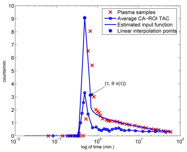
Comparison of the arterial plasma samples (crosses), average CA-ROI region time activity curve (solid line with open circles) and estimated input function solid line with 3 discrete asterisks. Also illustrated, with the 3 asterisks, is the time at which the average tracer activity is initiated in the CA-ROI τ₀, the time point for the peak value τ_p, the point of continuity τ between windows W₁ and W₂, and the three plasma samples used for the fit. Time is expressed on logarithm scale hence emphasizing the effects for early time.

After the early interval of roughly one half minute, image-derived data are subject to greater contamination of tracer spillover from tissue to blood. We therefore model the input data after the initial interval without using image-derived data, but using a limited number of intravenous plasma samples. The piecewise-continuous parameter-dependent formulation for the estimated input function u_e is given by

$$u_{\mathrm{e}}(t,\theta ,\lambda ,\delta )=\{\begin{array}{cc}0\hfill & t\in [0,{\tau }_0]\hfill \\ \theta v_p\frac{t-{\tau }_0}{{\tau }_p-{\tau }_0}\hfill & t\in [{\tau }_0,{\tau }_p]\hfill \\ \theta \frac{v_{\tau }(t-{\tau }_p)+v_p(\tau -t)}{\tau -{\tau }_p}\hfill & t\in [{\tau }_p,\tau ]\hfill \\ \theta v_{\tau }{e}^{-\lambda {(t-\tau )}^{\delta }}\hfill & t>\tau .\hfill \end{array}\phantom{\}}$$ (1)

Here the interval [0,τ] defines the early time window W₁ typically τ < 0.6 minutes and W₂ = [τ, T] is the second window, T ≈ 60 minutes. The parameter θ is introduced to account for partial volume effects and hematocrit in the measurement of the tracer concentration in v(t).

2.2 Image-derived input function data

The curve associated with the image data from CA-ROIs is obtained from the PET frames using the same protocol, and code as used in [9]. The initial time frames up to time 2 minutes are summed so as to emphasize those voxels which show the tracer in the CA-ROIs, typically 3 to 5 slices in the lower portion of the brain (for FDG-PET data acquired with the 951/31 EC AT scanner), and from which whole blood time activity curves for each observed CA-ROI can be calculated. Averaging over these curves yields the data that defines the average whole blood time activity curve v(t), see the solid line with open circles, Figure 1. We can see that v(t) provides crucial subject and situation dependent information on the input function, by providing the times at which the tracer reaches the CA-ROI, τ₀, and then the time at which it peaks in the blood, τ_p. The delay between u_p and v(t) is merely indicative of the shift due their measurement from different sources. An immediate visual comparison shows the underestimation of v(t) as compared to u_p(t), due to partial volume effects and hematocrit, which is accounted for in (1) through the scaling of v(t) inversely proportionally to its recovery from the image by parameter θ.

2.2.1 Piecewise linear approximation to the image-derived data for early time

Given the image-derived data for v(t), a piecewise linear approximation for v defined in model (1) which depends on the automatic selection of the three time points (τ₀,τ_p,τ). It is easy to determine τ_p as the point in the sampled data at which the highest intensity value v_p = v(τ_p) is achieved. The point τ_o provides an estimate of the initiation time of activity, prior to which there is effectively no signal, [14]. To facilitate the automatic estimation of τ_o we selected it as the point after which v(t) remains greater than .02v_p.

The significance of the time point τ, which is a time point shortly after τ_p, is to assure that the input on W₁ can be well approximated by two line segments and on W₂ it can be well-modeled by model u_w2 = θv_τe^{−λ(t−τ)δ}, see further details comparing this analytic form with other analytic expressions in [15]. While it can be determined automatically, it can not be simply predetermined to be a fixed number of points after the peak because noise may contaminate a chosen point. We chose, therefore, a relatively simple automatic way to select τ. Two straight line least squares fits are used. We form one linear data fit through the points τ_p and the next two points to the right of τ_p, and a second linear data fit through the last of these and two more to the right. Their point intersection defines both τ and the value v_τ, which is most likely not one of the discrete values of v(t).

3 Method

A nested optimization method for recovering the input function u_e(t) and the kinetic rate parameters of representative TTACS obtained from clustering is presented. The recovered u_e can then be used to calculate kinetic parameters and

$$K=\frac{K_1{k}_3}{k_2+k_3}$$ (2)

for additional TTACs.

3.1 Clustering the PET data

The fast clustering method described in detail in [13] is utilized to find p representative TTACs , $y_{\mathrm{TAC}}^{\left(i\right)}\left(t\right)$, i = 1 ⋯, for the whole brain excluding non-brain, blood vessel and CSF regions. Throughout we use superscript (i) to label cluster i, and assume that the cluster labeling is ordered such that the first cluster is the largest. The advantage of clustering is that it provides an automated way in which to segment the data into tissue groups of similar functional activity.

3.2 An algorithm for recovering the input function

In the compartmental model [16] for FDG-PET, the ideal TTAC y(t) at a given voxel, or for a specific brain tissue ROI, is given analytically by convolution (⊗) of the instantaneous response function (IRF) with input u(t)

$$y\left(t\right)=u\left(t\right)\otimes \left(\frac{K_1{k}_3}{k_2+k_3}+\frac{K_1{k}_2}{k_2+k_3}{e}^{-(k_2+k_3)t}\right).$$ (3)

The IRF is the term within the parentheses and depends on the specific tissue response to the tracer. K₁ is the transport rate from plasma to brain tissue with units ml/100g/minute, k₂ is the transport rate back from brain to blood vessel with units 1/minute, k₃ is the phosphorylation rate of intra-cellular FDG by hexokinase enzymes to FDG-6-phosphate with units 1/minute. Because the scanning interval 60 minutes is relatively small, it will be difficult to accurately estimate the dephosphorylation rate of intra-cellular FDG-6-phosphate back to FDG, k₄, [17]. We thus set k₄, which is itself small, to zero.

Typically, kinetic parameters for cluster curve y⁽ⁱ⁾, given by (3), can be obtained by the minimization of Φ⁽ⁱ⁾,

$${\Phi }^{\left(i\right)}({\mathbf{x}}^{\left(i\right)},{\alpha }^{\left(i\right)})=\sum _{j=1}^n{w}_j{\left(y_{\mathrm{TAC}}^{\left(i\right)}\left(t_j\right)-{\alpha }^{\left(i\right)}\cdot y^{\left(i\right)}\left(t_j\right)-(1-{\alpha }^{\left(i\right)})\cdot u\left(t_j\right)\right)}^2.$$ (4)

α⁽ⁱ⁾ accounts for both partial volume and spillover effects for cluster i, and the rate constants are components of ${\mathrm{x}}^{\left(i\right)}=[K_1^{\left(i\right)},k_2^{\left(i\right)},k_3^{\left(i\right)}]$. The contributions from each time point are weighted by w_j. Ideally, these are the inverse of the variances of the data of each frame and are different for different tissue TACs. Because of the difficulty of estimating the variances they are set to the time durations of the relevant time frames as practiced in [18]. To define a feasible space for the parameters bound constraints are imposed.

It is usually assumed that the values for u(t_j) used in (4) are measured values of the input function. In contrast, we intend the use of the functional form (1). With respect to the dominant first cluster, the parameters θ, λ, δ of the input function u_e(t) can be recovered simultaneously with the kinetic rate constants. This is accomplished in a two-stage process. Specifically, notice that for any given value of θ parameters λ, δ can be obtained as the solutions of

$$[\lambda \left(\theta \right),\delta \left(\theta \right)]={\mathrm{argmin}}_{\lambda ,\delta }\sum _{l=1}^3{\left[\theta v\left(\tau \right)e^{-\lambda {({\stackrel{\sim }{t}}_l-\tau )}^{\delta }}-u_{\mathrm{p}}\left({\stackrel{\sim }{t}}_l\right)\right]}^2,$$ (5)

using three intravenous plasma samples, $({\tilde{t}}_l,u_{\mathrm{p}}\left({\tilde{t}}_l\right))$, l = 1, 2, 3. Therefore, at each iteration in the minimization of Φ⁽¹⁾ (x⁽¹⁾, α⁽¹⁾), θ), noting now the introduced dependence on the recovery coefficient θ, (5) can be solved to obtain the updates of λ and δ.

To make the estimation of the input function more robust, we note that the input function is common to all TTACs and thus propose that the optimization be performed simultaneously over p clusters with cost function

$$\Phi (\mathbf{x},\alpha ,\theta )=\sum _{i=1}^p{\Phi }^{\left(i\right)}({\mathbf{x}}^{\left(i\right)},{\alpha }^{\left(i\right)},\theta )$$ (6)

where x = (x⁽¹⁾ ,…, x^(p)), and α = (α⁽¹⁾,…, α^(p)).)

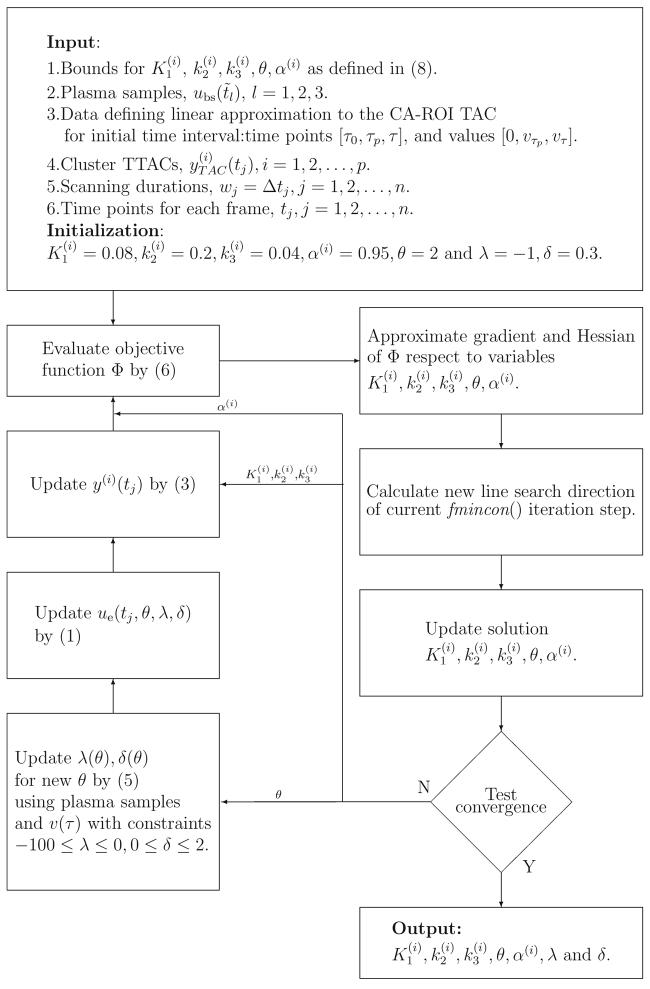
In summary, the nested optimization method, illustrated in the flow chart provided in Figure 2, is formulated as follows

$$\underset{\mathbf{x},\alpha ,\theta }{\min }\Phi (\mathbf{x},\alpha ,\theta )\text{subject to constraints}$$ (7)

$$\begin{array}{c}\hfill 1.2\le \theta \le 4,0.9\le {\alpha }^{\left(i\right)}\le 1,\hfill \\ \hfill 0.015\le K_1^{\left(i\right)}\le 0.3,0.024\le k_2^{\left(i\right)}\le 0.54,0.01\le k_3^{\left(i\right)}\le 0.2.\hfill \end{array}$$ (8)

Matlab 7.0 function fmincon from the optimization toolbox version 3.0.2 [19] utilized for carrying out this constrained minimization. The bounds used are based on experimental results [17] for both gray and white matter from 13 but with doubling of upper bounds and halving of lower bounds such that the feasible space is not too conservatively estimated. Time delay between the TTACs and the input function is removed by automatically shifting the TTACs such that the first peak of each is aligned with v_τp.

Fig. 2.

Flow chart detailing the steps of the nested optimization.

4 Results

Experiments are reported which assess the method with respect to the number of clusters, visually examine the recovered input function as compared to plasma-sampled data, demonstrate the robustness of the parameters defining the input function, use the recovered input function in graphical Patlak analysis as compared to using the plasma-sampled data, and compare the calculation of (2) using the kinetic parameters obtained by nonlinear least squares for both plasma-sampled input data and the recovered input function.

4.1 Clinical data set

The retrospective PET data available were collected using a 951/31 ECAT scanner (Siemens, Knoxville, TN) with the identical scanning protocol for each subject. An initial 20 minutes transmission scan was acquired for attenuation correction and an intravenous bolus of 10 mCi FDG administered over 5-10 seconds under resting condition. PET images were reconstructed using a filtered back projection algorithm with Hanning filter of 0.40 cycles per voxel. There are 31 transaxial slices of 128 × 128 voxels, each voxel of size 0.18776 × 0.18776 cm², with a center-to-center slice separation of 3.375 mm and a 10.8 cm axial field of view. The final reconstructed PET images have an in-plane resolution of 9.5 mm full-width at half maximum (FWHM) in the center of the field of view and an axial resolution of 5.0-7.1 mm FWHM. Scanning durations, given in minutes, for the reconstructed frames were 0.2, 8 × 0.0333, 2 × 0.1667, 0.2, 0.5, 2 × 1, 2 × 1.5, 3.5, 2 × 5, 10 and 30. (The noisy first frame is excluded from the analyses.) Total session duration was 60 minutes. The arterial plasma samples were drawn every 5 seconds for the first minute, every 10 seconds for the second minute, every 30 seconds for the next 2 minutes, and then at 5, 6, 8, 10, 12, 15, 20, 25, 30, 40, 50 and 60 minutes, yielding a discrete representation of the plasma sampled function with units counts/ml/minute, denoted by u_p(t_j), for j = 1,… ,34.

4.2 Dependence on the number of clusters

Utilizing a greater number of cluster TTACs in minimizing the cost function (7) increases the computational complexity. To assess the dependence on p of the recovered input, and resulting estimated K by (2), the nested optimization of the constrained cost function is solved using p = 1, 2, and 3 clusters, out of a total of 5 clusters. The recovered input u_e for each choice of p, namely u_e with the converged values for θ, λ and δ, is then used in standard nonlinear fitting for estimating the tissue kinetic rates and vascular fraction for each cluster TTAC i of the brain volume clustered to a total of 50 clusters. Results are compared with those obtained using plasma sampled data in place of u_e in the nonlinear fitting.

Linear regression analysis for the estimates of K performed for all 18 subjects and 50 clusters is illustrated in Figure 3. The measurements of K are highly comparable for all choices of p; correlation coefficients .97968, .99269 and .99115, slopes near one .9735, .9832, .9873 and intercepts around zero, .0012, 00096, and .00074, in each case for p = 1, 2 and 3. Figure 3 illustrates the inferiority for p = 1 and that p = 2 and p = 3 are comparable. Thus we suggest using p = 2 to minimize cost, without affecting the quality. All other reported results use p = 2.

Fig. 3.

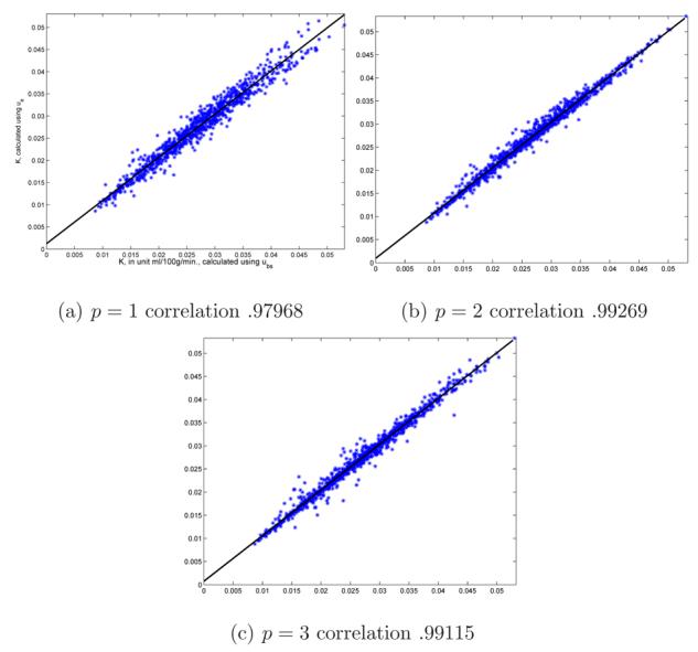
Linear regression for parameter K, calculated by (2), with u_p as compared to u_e obtained using 1, 2 and 3 clusters. Regression is carried out over 50 clusters for all 18 subjects.

4.3 Visual inspection of the input function

A comparison of the estimated input function u_e with the plasma-sampled input u_p is illustrated in Figure 4. Because these two curves come from different sources, namely CA-ROI and arm arterial plasma samples, there is a time shift between them. In order to provide a better comparison u_e is automatically shifted to match u_p, see Figure 4 (b). As expected the tails of both curves are closer because the tail of the estimated curve is obtained by the fit with the plasma samples. For all subjects u_e is smoother for later time because it is evaluated using a functional form. Additional representative comparisons of u_p with shifted u_e are shown in Figure 5.

Fig. 4.

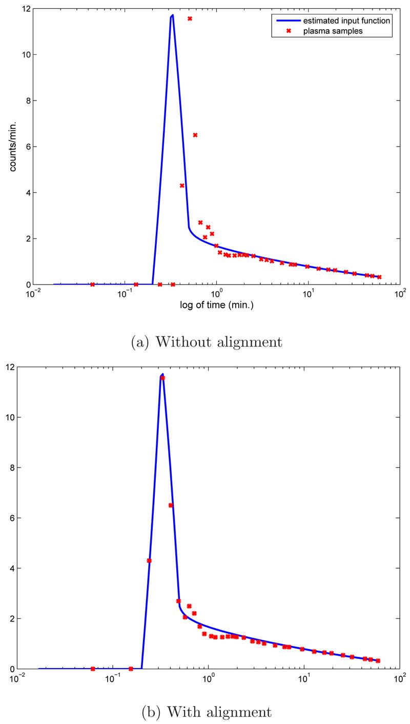
The recovered input function u_e(t) compared with arterial plasma samples, u_p(t). Illustrated are the data given on logarithm time scale (a), and (b) the same data with u_e(t) shifted to account for the time delay relative to u_p(t).

Fig. 5.

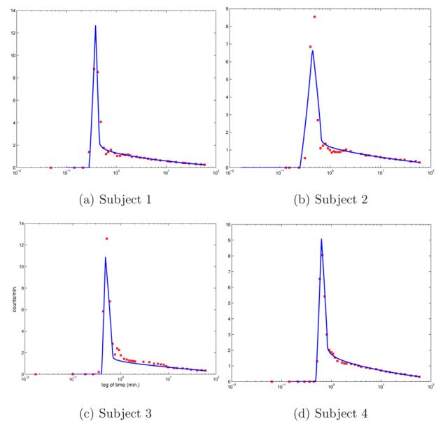
Comparison of shifted estimated input u_e, continuous line, and u_p for representative subjects, 1 – 4, in (a)-(d).

4.4 The model parameters defining u_e

Table 1 presents the estimates for θ, λ and δ. The consistency of δ around the average of 0.248 suggests the robustness of model u_W2 with respect to different subjects. We observe that α⁽ⁱ⁾ are remarkably consistent across all subjects and clusters, and well within the range prescribed by the constraints. On the other hand, the variation in θ is indicative of the variable partial volume effects because the identified CA-ROIs vary in their location, size and shape between subjects.

Table 1.

Constants α⁽ⁱ⁾ (7) of each cluster and parameters defining u_W2 obtained in the proposed method.

Subject	θ	λ	δ	α(1)	α(2)
1	2.049	0.923	0.233	0.930	0.931
2	1.975	0.805	0.226	0.923	0.927
3	2.843	0.691	0.241	0.935	0.935
4	2.730	0.872	0.237	0.958	0.957
5	1.790	0.518	0.318	0.912	0.915
6	2.294	0.828	0.265	0.938	0.932
7	2.287	0.350	0.364	0.928	0.929
8	3.190	0.797	0.257	0.935	0.934
9	2.927	0.919	0.231	0.953	0.968
10	2.813	1.554	0.153	0.918	0.927
11	2.651	0.521	0.342	0.933	0.932
12	2.246	0.628	0.247	0.930	0.925
13	3.543	0.781	0.277	0.941	0.941
14	1.908	0.937	0.212	0.941	0.940
15	3.781	0.792	0.257	0.942	0.940
16	2.822	1.152	0.167	0.935	0.935
17	3.070	0.924	0.214	0.951	0.944
18	2.996	0.842	0.222	0.947	0.924
Average	2.662	0.824	0.248	0.936	0.935

4.5 Quantitative evaluation for real data by Patlak analysis

To provide a comparison with the method presented in [9], the recovered input for each subject is used in Patlak analysis for each cluster TTAC. The data of the last three frames, i.e. 15 min. to 60 min., are used for the Patlak analysis. The equilibrium of the FDG tracer in this time interval is justified in [20]. Results are compared with those obtained using the plasma sampled data, see Table 2 for representative results for the first 5 subjects. The calculated K over all clusters and all subjects are highly correlated, correlation coefficient 0.99686, slope 0.9878 and intercept .00071, see Figure 6. The within subject variation of K is comparable whether calculated using u_p or u_e. The results are comparable to those presented in [9], in which analysis of CMRglc for one subject yields R² .9997, slope 1.0018, and intercept −0.031.

Table 2.

Linear regression analysis comparing calculation of K by Patlak analysis using input functions u_p and u_e, for cluster TTACs for representative subjects.

Subj.	up mean K ± std. dev.	ue mean K ± std. dev.	Corr. Coeff.	Slope	Intercept
1	.033963 ± .007409	.034371 ± .007466	.99996	1.008	.00015
2	.024923 ± .004949	.026501 ± .005065	.99887	1.022	.00130
3	.023531 ± .005635	.024157 ± .005797	.99997	1.029	−.00005
4	.026678 ± .003745	.026811 ± .003745	.99991	1.000	.00013
5	.030645 ± .005961	.030775 ± .005870	.99945	0.984	.00061

Fig. 6.

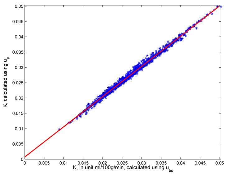
Linear regression for K calculated with u_p as compared to u_e using Patlak analysis. Regression analysis for all subjects and all clusters yields high correlation 0.99686, with slope .9878 and intercept .00071.

4.6 Quantitative evaluation for real data by nonlinear least squares

To further evaluate the method of Section 3 for recovering the input function it is used in the postestimation of K₁, k₂ and k₃, and in turn K, and these values compared to those in which the plasma-sampled data is used. Table 3 provides the results of linear regression analysis, the slopes, intercepts and correlation coefficients for the calculation of K for first 5 subjects over all 50 clusters. Again, the within subject variation of K is comparable whether calculated by u_p or u_e. Figure 7 illustrates the regression analysis for individual kinetic rate parameters K₁, k₂ and k₃ for subject 5.

Table 3.

Linear regression analysis comparing calculation of K by (2) using input functions u_p and u_e, for cluster TTACs for representative subjects.

Subj.	up mean K ± std. dev.	ue mean K ± std. dev.	Corr. Coeff.	Slope	Intercept
1	.031580 ± .010040	.032050 ± .009939	.99708	0.987	.00089
2	.025624 ± .006794	.027106 ± .006846	.99661	1.004	.00140
3	.023363 ± .007258	.023972 ± .007333	.99226	1.002	.00055
4	.025738 ± .005860	.025944 ± .005823	.99940	0.993	.00038
5	.029736 ± .007804	.029685 ± .007336	.98896	0.930	.00230

Fig. 7.

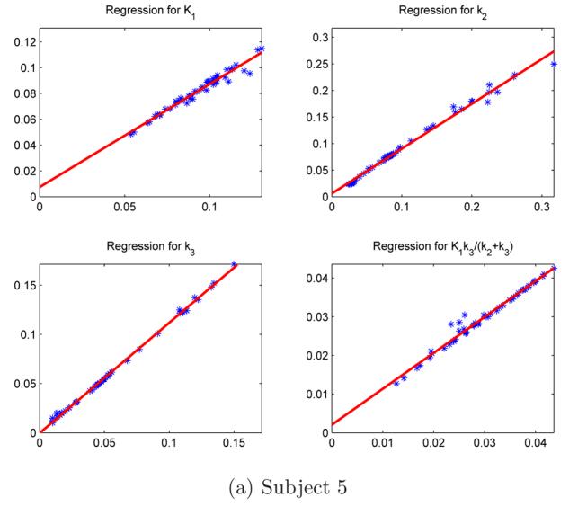
Comparing the two sets of parameters calculated by u_e, x-axis, and u_p, y-axis, for subject 5. The correlation coefficients of these four parameters are 0.98140, 0.99538, 0.99916 and 0.98896.

Although not presented here, a careful examination of results obtained with u_e (u_p), respectively, shows that in only 2(0), 8(8) and 34(24) cases out of 900 were the bounds K₁, k₂ and k₃, attained, which justifies the choice of bounds for the rate constants in the optimization problem.

4.7 Quantitative validation of u_e for simulated data

Kinetic rate parameters, K₁, k₂, k₃ for the first three sets of both gray and white materials from Table 1 in [17] are used for simulation. For each set of rate parameters we obtain a TTAC using convolution equation (3) with u_p substituted for u(t). This yields 6 TTACs with known rate parameters and K for each subject. Then the subject-dependent recovered u_e was used to estimate K by graphical Patlak analysis and directly from (2) using the recovered kinetic parameters obtained by weighted nonlinear least squares. This process studies the use of u_e in the postestimation stage for the 50 clusters for each subject, as described in Section 4.6, but with data for which the exact K is known.

The calculated K for all simulation data are well-correlated with the true values, correlation coefficients are .96213 and .99780, slopes are .9943 and 1.019, and intercepts .0015, −.000047, for the calculation of K by Patlak analysis and directly using (2), resp. The mean and standard deviation of the relative estimation errors of K are 5.481% (1.676%) and 7.766% (0.301%). The individual rate parameters are quite well correlated, with correlation coefficient and slope pairs for K₁, k₂ and k₃ (.94319, 1.076), (.89782, 1.083), and (.95925, 1.006), resp.

5 Discussion

Here we focus on certain specifics of the method described in Section 3.

5.1 Recovering the input function

In the model of the input for u_e the values v_τp and v_τ are known and only the three parameters, θ, λ and δ, need to be determined. Rather than using the TTACS to obtain the parameters of this input function, these could be obtained by directly fitting the model u_W2 with three plasma samples. In that case, the analytic form for u_W2 could be extrapolated to provide values for t ≥ τ, with scaling by θ of the linear parts in (1) for 0 < t ≤ τ. In Figure 8 we illustrate for one subject the recovered input function that is obtained by the algorithm described in Section 3 as compared to that obtained directly by data fitting with just the plasma samples and extrapolation. This shows that without information from the TTACs, the data on the early time window are shifted too high, θ = 3.909.

Fig. 8.

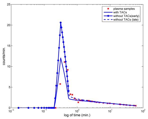
Comparing the recovered input function by direct data fitting of the plasma samples (θ = 3.909) and by using the TTACS in the data fitting (7) (θ = 2.287), for representative subject 7. The use of the TTACS in the nested optimization yields a θ which leads to a much better fit of the recovered input function with the plasma samples.

5.2 Time shift between plasma samples and the image-derived time activity curve

As we can see from Figures 1 and 4, there is always a time shift between the CA-ROI TAC and the measured plasma samples for early time. Should the data on W₁ measured from the CA-ROI be shifted to match with that on W₂ which is obtained directly from the three plasma samples? We used the arterial plasma samples to determine that the actual shift for subject 4 is 10 seconds. The plasma samples at approximate times 10, 30 and 60 minutes are 0.7150, 0.4487, 0.3130 counts/ml/minute, resp. Supposing all plasma samples for t > τ are shifted by 10 seconds to the right and then used in the fit for u_W2, the differences at these same three time points are just −.004, −.001, −.0005, resp. with relative errors less than 0.56%. It has been reported that the impact of errors of this magnitude in the input function is insignificant in terms of parametric estimation, [21]. We conclude that the shift of W₁ relative to W₂ is negligible.

5.3 Plasma Sampling

In this study we took advantage of the availability of arterial plasma samples to assess all aspects of the method, using the validated compatibility between arterial and venous plasma samples, with less than 2.25% mean difference over all time points, [9]. Practically, for new studies in which arterial sampling is not already intended, the use of venous, rather than arterial samples, as described also in [9] is recommended as a less invasive and less painful method of acquiring the necessary data.

5.4 Advantage of utilizing two windows in defining the input function

In the proposed method we introduced the use of two windows for defining u_e because of the difficulty that arises in finding a single analytic formulation which can give a good model for the tracer concentration in plasma for the entire time duration. The use of the two windows provides more flexibility and less complexity for modeling u_e after the initial half minute, and the first half minute is easily approximated. This approximation on W₁ is a crude simplification, but it is a very good approximation to the real process when τ is very small. Clearly, it is also possible to use higher order fitting [4] rather than linear approximation on W₁ but with τ < 0.6 minute the impact will be insignificant. On the other hand, for later time the image derived CA-ROI TAC may be contaminated by spillover and so three samples are utilized to replace the CA-ROI data. As compared to other image-based input function estimation methods, [10], [22], [9], [11], [23], [12], which use the entire CA-ROI TAC for recovery of the input data, the proposed method is free from spillover contamination at later time.

6 Conclusions

A reliable semi-automated alternative for input function estimation which uses image-derived data augmented with 3 plasma samples has been presented and validated for FDG-PE T human brain studies. A simulated data study validates the recovered input for finding known kinetic values. In contrast to the original method proposed in [9], there is no need to additionally manually determine the tissue region of interest near the CA-ROI. The Matlab-based implementation of the tool is available at web site http://math.asu.edu/~rosie/guo/inpfest_pub.tar.gz.

References

- 1.PET-Working Group PET Working Group: NIH/NIA Neuroimaging Initiative. 2005 URL http://www.nia.nih.gov/ResearchInformation/ExtramuralPrograms/NeuroscienceOfAging/Summary+%E2%80%93+PET+Working+Group.htm .
- 2.Phelps ME, Huang S-C, Hoffman EJ, Selin CE, Kuhl D. Tomographic measurement of local cerebral glucose metabolic rate in man with (18F) fluorodeoxyglucose: Validation of method. Ann. Neurol. 1979;6:371–388. doi: 10.1002/ana.410060502. [DOI] [PubMed] [Google Scholar]
- 3.Bentourkia M. Kinetic modeling of PET-FDG in the brain without blood sampling. Comp. Med. Imag. Graph. 2006;30:447–451. doi: 10.1016/j.compmedimag.2006.07.002. [DOI] [PubMed] [Google Scholar]
- 4.Eberl S, Anayat AR, Fulton RR, Hooper PK, Fulham MJ. Evaluation of two population based input functions for quantitative neurological FDGPET studies. Eur. J. Nucl. Med. 1997;24:299–304. doi: 10.1007/BF01728767. [DOI] [PubMed] [Google Scholar]
- 5.Tsuchida T, Sadato N, Yonekura Y, Nakamura S, Takahashi N, Sugimoto K, et al. Noninvasive measurement of cerebral metabolic rate of glucose using standardized input function. J. Nuc. Med. 1999;40(9):1441–1445. [PubMed] [Google Scholar]
- 6.Riabkov DY, Bella EVRD. Estimation of kinetic parameters without input functions: Analysis of three methods for multichannel blind identification. IEEE Trans. Biomed. Eng. 2002;49(11):1318–1327. doi: 10.1109/TBME.2002.804588. [DOI] [PubMed] [Google Scholar]
- 7.Feng DG, Wong K-P, Wu C-M, Siu W-C. A technique for extracting physiological parameters and the required input function simultaneously from PET image measurements: Theory and simulation study. IEEE J. ITBM. 1997;1(4):243–254. doi: 10.1109/4233.681168. [DOI] [PubMed] [Google Scholar]
- 8.Wong K-P, Feng D, Meikle SR, Fulham MJ. Simultaneous estimation of physiological parameters and the input function - In vivo PET data. IEEE J. ITBM. 2001;5(1):67–76. doi: 10.1109/4233.908397. [DOI] [PubMed] [Google Scholar]
- 9.Chen K, Bandy D, Reiman E, Huang S-C, Lawson M, Feng D, et al. Noninvasive quantification of the cerebral metabolic rate for glucose using positron emission tomography, 18F-fluorodeoxyglucose, the Patlak method, and an image-derived input function. J. Cereb. Blood Flow Metab. 1998;18:716–723. doi: 10.1097/00004647-199807000-00002. [DOI] [PubMed] [Google Scholar]
- 10.Litton J-E. Input function in PET brain-studies using MRI defined arteries. J. Comp. Ass. Tom. 1997;21(6):907–909. doi: 10.1097/00004728-199711000-00012. [DOI] [PubMed] [Google Scholar]
- 11.Wahl LM, Asselin MC, Nahmias C. Regions of interest in the venous sinuses as input functions for quantitative PET. J. Nucl. Med. 1999;40(10):1666–1675. [PubMed] [Google Scholar]
- 12.Asselin MC, Cunningham VJ, Amano S, Gunn R, Nahmias C. Parametrically defined cerebral blood vessels as non-invasive blood input functions for brain PET studies. Phys. Med. Biol. 2004;49(6):1033–54. doi: 10.1088/0031-9155/49/6/013. [DOI] [PubMed] [Google Scholar]
- 13.Guo H, Renaut RA, Chen K, Reiman E. Clustering huge data sets for parametric PET imaging. Biosystems. 2003;71(12):81–92. doi: 10.1016/s0303-2647(03)00112-6. [DOI] [PubMed] [Google Scholar]
- 14.Raichle ME, Martin WR, Herscovitch P, Mintun MA, Markham J. Brain blood flow measured with intravenous 15O-H2O II. Implementation and validation. J. Nucl. Med. 1983;24:790–798. [PubMed] [Google Scholar]
- 15.Guo H, Renaut R, Chen K. Evaluating an alternative model for the input function in FDG-PET studies. 2007 URL http://math.la.asu.edu/~rosie/mypapers/nmbsupp.pdf.
- 16.Sokoloff L, Reivich M, Kennedy C, Rosiers MHD, Patlack CS, Pettigrew KD, et al. The [14C] deoxyglucose method for the measurement of local cerebral glucose metabolism: theory procedures and normal values in the conscious and anesthetized albino rat. J. Neurochem. 1977;28:897–916. doi: 10.1111/j.1471-4159.1977.tb10649.x. [DOI] [PubMed] [Google Scholar]
- 17.Huang S-C, Phelps ME, Hoffman EJ, Sideris K, Selin CJ, Kuhl DE. Noninvasive determination of local cerebral metabolic rate of glucose in man. Am. J. Physiol. 1980;238(E):69–82. doi: 10.1152/ajpendo.1980.238.1.E69. [DOI] [PubMed] [Google Scholar]
- 18.Zhou Y, Endres CJ, Brasic JR, Huang S-C, Wong DF. Linear regression with spatial constraint to generate parametric images of ligand-receptor dynamic PET studies with a simplified reference tissue model. NeuroImage. 2003;18(4):975–989. doi: 10.1016/s1053-8119(03)00017-x. [DOI] [PubMed] [Google Scholar]
- 19.The Mathworks Optimization Toolbox User's Guide. 2005 [Google Scholar]
- 20.Wienhard K, Pawlik G, Herholz K, Wagner R, Heiss W-D. Estimation of local cerebral utilization by positron emission tomography of 18F-2-fluoro-2-deoxy-d-glucose: a critical appraisal of optimization procedures. J. Cereb. Blood Flow Metab. doi: 10.1038/jcbfm.1985.15. [DOI] [PubMed] [Google Scholar]
- 21.Chen K, Huang S-C, Yu D-C. The effects of measurement errors in the plasma radioactivity curve on parameter estimation in positron emission tomography. Phy. Med. Biol. 1991;36(9):1183–1200. doi: 10.1088/0031-9155/36/9/003. [DOI] [PubMed] [Google Scholar]
- 22.Liptrot M, Adams KH, Martiny L, Pinborg LH, Lonsdale MN, Olsen NV, et al. Cluster analysis in kinetic modelling of the brain: A noninvasive alternative to arterial sampling. Neuroimage. 2004;21(2):483–493. doi: 10.1016/j.neuroimage.2003.09.058. [DOI] [PubMed] [Google Scholar]
- 23.Sanabria-Bohorquez SM, Maes A, Dupont P, Bormans G, de Groot T, Coimbra A, et al. Image-derived input function for [11C] flumazenil kinetic analysis in human brain. Mol. Imag. Biol. 2003;5(2):72–78. doi: 10.1016/s1536-1632(03)00046-5. [DOI] [PubMed] [Google Scholar]