Power and Sample Size Calculation for Neuroimaging Studies by Non-Central Random Field Theory

Abstract

Determining power and sample size in neuroimaging studies is a challenging task because of the massive multiple comparisons among tens of thousands of correlated voxels. To facilitate this task, we propose a power analysis method based on random field theory (RFT) by modeling signal areas within images as non-central random field. With this framework, power can be calculated for specific areas of anticipated signals within the brain while accounting for the 3D nature of signals. This framework can also be extended to visualize local variability in sensitivity as a power map and a sample size map. We validated our non-central RFT framework based on Monte-Carlo simulations. Moreover, we applied our method to a blood oxygenation level dependent (BOLD) functional magnetic resonance imaging (fMRI) data set with a small sample size in order to demonstrate its use in study planning. From the simulations, we found that our method was able to estimate power quite accurately. In the fMRI data analysis, despite the small sample size, we were able to determine power and the number of subjects required to detect signals.

Introduction

When planning biomedical studies, investigators have to consider two seemingly paradoxical facts. It is important to have a sufficiently large number of subjects to detect the signal or effect of interest. On the other hand, it is also important to include as few subjects as possible in order to avoid unnecessarily exposing subjects to unforeseen risks and to reduce the costs associated with the study. Therefore, determining the appropriate number of subjects is an important step in study planning. This process of power analysis is straightforward in studies with a single outcome variable (Cohen 1988), and a number of software tools are widely available for such single-outcome power analyses. In neuroimaging studies, however, power calculation is a complicated process due to the fact that outcomes are in the form of 3D images with tens of thousands of correlated voxels. Hence simply applying the single-outcome power analysis may not be appropriate for neuroimaging data.

Compared to the development of statistical inference methods, relatively little effort has been focused on the development of power analysis methods in neuroimaging data. Nevertheless there have been some attempts in calculating power for neuroimaging studies. Theoretical work started as early as the application of RFT (random field theory) to neuroimaging data. Friston et al. (1994) modeled signals in a statistic image as a Gaussian random process, and produced a power surface by expressing power as a function of the threshold height and signal width. This was later used to discuss power (Friston, et al. 1996) and sample sizes (Friston, et al. 1999) in neuroimaging data analyses from a theoretical perspective. However, this relatively simple method was unable to calculate power to detect signals at a specific location within the brain. Rather, this method calculated power to detect signals in random locations anywhere in the brain, not necessarily at the location where the investigator anticipated. In another RFT-based approach, Siegmund and Worsley (1995) described the behavior of power to detect a single Gaussian-shaped signal with unknown location in the search region. Although this is a typical signal considered in the RFT literature, this may not accurately represent signals with multiple foci often detected in neuroimaging data.

Besides RFT, others have taken a different approach and extended the single-outcome power analysis to neuroimaging data. The main idea of such an approach is to calculate power based on a non-central distribution at each voxel. Van Horn et al. (1998) used a non-central F-distribution to calculate power at each voxel. Although they were unable to account for spatial correlation and multiple comparisons in their power analysis, they were able to produce a power map, an image describing the spatial variability of power in different areas of the brain. Zarahn and Slifstein (2001) used a non-central T-distribution to calculate power, using a rudimentary multiple comparison correction with the Bonferroni method. One shortcoming of this type of power analyses is that the method focuses on power at each voxel separately and ignores the spatially correlated nature of signals. If a signal is observed in one voxel, then it is likely to be observed in the neighboring voxels as well due to spatial correlation. Thus it is more appropriate to calculate power for a collection of voxels, rather than at each single voxel separately.

Simulation and resampling-based methods are other conventional approaches to calculate power. Although computationally intensive, such methods have been applied to neuroimaging studies. Desmond and Glover (2002) predicted power in fMRI studies based on simulations, and produced power curves to summarize their results. Their work has been referenced often in the neuroimaging community for power and sample size issues. Murphy and Garavan (2004) used a resampling technique to calculate power based on their data set. It should be noted that neither of the above studies corrected for multiple comparisons. Rather, very high uncorrected thresholds (p<0.000002 in Desmond and Glover (2002) and p<0.000001 in Murphy and Garavan (2004)) were chosen in order to account for a large number of voxels involved in statistical inference. Moreover, to obtain a power curve or a sample size curve by these methods, the simulation or resampling process needs to be repeated for different degrees of freedom (df), requiring a considerable amount of time and computing resources. Such a process is very impractical for neuroimaging investigators.

To overcome the problems described above, we propose a new power analysis method specifically designed for neuroimaging data. In particular, we present a power analysis method based on RFT for non-central random fields. Analogous to non-central random variables used to describe signals in single-outcome power analyses, non-central random fields are used to describe signals in statistical images. We refer to this new approach as the non-central RFT framework. An RFT-based parametric framework is chosen because of its computational efficacy; the distribution of the test statistic can be modeled by a single parametric model (Cao and Worsley 2001; Worsley, et al. 1996b). Power calculated by this framework is adjusted for multiple comparisons while accounting for spatial correlation among voxels. The non-central RFT framework can account for the effect size as well as the spatial characteristics of anticipated signals (extent and topology), allowing investigators to explicitly specify the alternative hypothesis in the power calculation. This means that users can calculate power in the areas where signals are anticipated rather than at random locations. We also extend this non-central RFT framework to visualize power in different parts of the brain in the form of a power map and a sample size map (Van Horn, et al. 1998). The resulting maps can aid investigators to determine where signals are likely to be detected and how many subjects are needed in their planned studies. In this paper, we validate the non-central RFT framework by simulations, and then apply it to a BOLD fMRI study to demonstrate its use.

Methods and Materials

Overview of the Non-Central RFT Framework

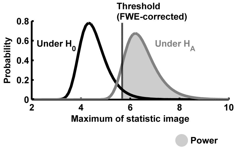
In principle, the non-central RFT framework is similar to any other power calculation methods. First, the distribution of the test statistic under the null hypothesis (H₀) is obtained, and then the distribution under the alternative hypothesis (H_A) is obtained. Once both distributions are found, then power can be obtained as the probability of detecting signals with the threshold controlling the significance level (see Figure 1). In a neuroimaging study, H₀ often corresponds to absence of signals (i.e., no difference or effect) in the entire brain, whereas H_A corresponds to presence of signals in some specific areas of the brain (e.g., visual cortices, auditory cortices, fusiform gyri, etc.). We describe a statistic image under H_A as patches of central and non-central random fields (see Figure 2). The distribution under H₀ corresponds to the distribution of the maximum of T- or F-random fields, which has been studied and documented extensively (Cao and Worsley 2001; Worsley 1994; Worsley, et al. 1992; Worsley, et al. 1996b). The distribution under H_A corresponds to the distribution of the maximum of non-central T- or F-random fields, respectively.

Figure 1.

A schematic of power calculation for neuroimaging data analysis. The figure shows two distributions of the maximum of the statistic image: one under H₀ and the other under H_A. Based on these distributions, power (shaded area) is calculated as the probability above the FWE-corrected threshold under H_A.

Figure 2.

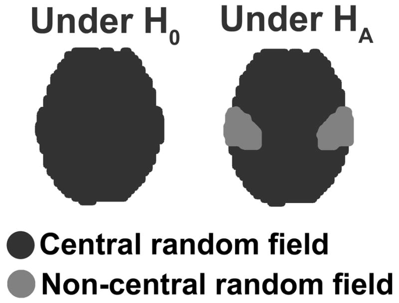
Under H₀, no signal is expected and the statistic image is modeled by a central random field. Under H_A, signals are expected in some known areas and the statistic image is modeled by patches of central and non-central random fields. The areas of anticipated signals are modeled by the non-central random field, whereas the areas of no signal are modeled by the central random field.

Non-Central Random Fields

A non-central T-field S with df=m and non-centrality (nc) =δ is defined as

$$S=\frac{\sqrt{m}(Z+\delta )}{\sqrt{V}}$$ (1)

where Z is a Gaussian random field with smoothness FWHM (full-width at half-maximum)=h, δ >0 is a scalar, and V is a chi-square random field with df=m. Note that V can be described as a squared sum of m independent Gaussian random fields with the same smoothness as Z (Adler 1980; Worsley 1994). A non-central F-field G with df=m,n and nc=η is defined as

$$G=\frac{\frac{1}{m}\left(U+{\left(Z+\sqrt{\eta }\right)}^2\right)}{\frac{1}{n}V}$$ (2)

where U is a chi-square random field with df = m −1, Z is a Gaussian random field, V is a chi-square random field with df=n, and η>0 is a scalar non-centrality parameter. All the random fields U, Z, and V have the same smoothness FWHM=h. A non-central field (1) or (2) can account for the effect size as well as the spatial correlation within the areas of anticipated signals. The distribution of the maximum for a non-central random field can be obtained from RFT.

Distribution of the Maximum by RFT

The distribution of the maximum is sought in statistical inference of neuroimaging data not only in RFT-based tests but also in permutation-based tests (Bullmore, et al. 1999; Holmes, et al. 1996; Nichols and Holmes 2002) in order to control the family-wise error (FWE) rate, or the probability of type I error in any voxel (Holmes, et al. 1996). In RFT, the distribution of the maximum of a statistic image is expressed by a parametric model. In particular, the probability of the maximum of a random field W exceeding a sufficiently high threshold u is approximated by

$$Pr\left(\underset{t\in A}{max}W(t)>u\right)\approx {\sum }_{i=0}^3{\mu }_i(A){\rho }_i(u)$$ (3)

where μ_i(A) is the i-dimensional RESEL (resolution element) count describing the i-dimensional spatial property of the search volume A (Cao and Worsley 2001; Worsley, et al. 1996b). In a 3D search volume, μ₃, μ₂, and μ₁ correspond to the volume, surface area, and diameter of the search volume in terms of RESELs, respectively. The 0-th term μ₀ corresponds to the Euler characteristic (EC) of the search volume. That is, the number of connected regions in the search volume minus the number of holes and hollows (Worsley 1996). The function ρ_i(u) is the i-dimensional RESEL density at the threshold u. It is determined by the underlying random field (e.g., Gaussian, T-, or F-random field), df, and the threshold u. The RESEL density ρ_i(u) for a number of random fields, including T- and F-random fields (Cao and Worsley 1999; Cao and Worsley 2001; Worsley, et al. 1996b), has been derived based on the first and second spatial derivatives (Cao and Worsley 2001; Worsley 1994) as briefly described in Appendix A. Detailed derivations of RESEL densities for central T- and F-random fields have been shown by Worsley (1994). We followed these derivations and extended them to non-central T- and F-random fields in (1) and (2). Details on this derivation are found in Hayasaka (2007). Appendix A shows the resulting RESEL densities for these non-central random fields. Note that, if the non-centrality parameter is zero, then these RESEL densities are identical to that of the corresponding central random field.

Power Based on the Non-Central RFT Framework

In order to calculate power, a threshold u_c controlling the FWE rate is sought first. This can be obtained from (3) by finding u_c at the significance level α (FWE-corrected) such that

$$\alpha =Pr\left(\underset{t\in A}{max}W(t)>u_c\mid H_0\right)\approx L=\sum _{i=0}^3{\mu }_i(A){\rho }_i(u_c)$$

where A is the entire search volume and W(t) is the value of the statistic image at voxel t ∈ A. In the SPM package (Wellcome Department of Imaging Neuroscience; London, UK), L above is transformed as

$$\alpha =Pr\left(\underset{t\in A}{max}W(t)>u_c\mid H_0\right)\approx 1-exp(-L).$$

This is due to the fact that L ≈ 1 − exp(L) when L is small. This transformation also restricts the probability estimates to be between 0 and 1.

Once the FWE-corrected threshold u_c is found, then power can be found based on (3) for the corresponding non-central random field. In order to do so, the alternative hypothesis needs to be explicitly defined by specifying the area of anticipated signal B ⊂A. For example, in Figure 2, the entire brain can be considered as A, whereas the light gray areas under H_A can be considered as B. The anticipated signal magnitude within B is described by a single non-centrality parameter nc=γ. Then, power λ can be obtained as the probability that the maximum of W(t) exceeds u_c under H_A. This is based on the rationale that, if the maximum within B exceeds u_c, then the hypothetical signal under H_A can be detected with this threshold. Power can be written as,

$$\lambda =Pr\left(\underset{t\in A}{max}W(t)>u_c\mid H_A\right)=Pr\left(\underset{t\in B}{max}W(t)>u_c\right)\approx 1-exp(-\stackrel{\sim }{L})$$ (4)

with

$$\stackrel{\sim }{L}=\sum _{i=0}^3{\mu }_i(B){{\rho }_i}^{\prime }(u_c;\gamma )$$ (5)

where ρ_i′ is the i-dimensional RESEL density for the non-central field (either non-central T- or F-field) with nc=γ. Note that the power estimated from (4) is corrected for multiple comparisons among voxels in B, and the threshold u_c is corrected for multiple comparisons for the entire search volume A.

The non-centrality parameter γ is closely related to, and easily estimated from, the effect size. In the non-central RFT framework, the effect size can be easily estimated from the average of the statistic image W(t) within B. When a one-sample T-test with df=m is to be used, then the effect size can be estimated in terms of Cohen’s d (Cohen 1988), and the non-centrality parameter can be calculated by $\gamma =d\sqrt{m}$. When an F-test with df=m,n is to be used, then the effect size can be estimated in terms of Cohen’s f (Cohen 1988) and the non-centrality parameter can be calculated by γ = (m + n + 1) f².

Special Considerations for Non-Central RFT Framework

The RFT-based statistical methods have been found to be conservative, especially when image data are not smooth or the df is small (Nichols and Hayasaka 2003; Worsley 2005). Such conservativeness is rarely a problem in statistical inference since the test is still able to control the FWE rate under the desired level of significance (Nichols and Hayasaka 2003), but this could lead to overestimation of power. It is difficult to theoretically determine how much this conservativeness influences power estimates, but we have found from our simulation-based validation that a small df offset can correct this problem. This ad-hoc adjustment is implemented by reducing the df used to calculate the corrected threshold u_c, the non-centrality parameter γ, and power relative to the original test. For a T-test with df=m, power is calculated with the adjusted df m′= m −m_p instead of m, where m_p is the df offset. Similarly for an F-test with df=m,n, power is calculated with the adjusted denominator df n′ = n −n_p instead of n, where n_p is the df offset. For low smoothness data (image FWHM < 10 voxels), a df offset of 2 is sufficient, and for sufficiently smooth data (FWHM > 10 voxels), a df offset of 1 seems to produce satisfactory results.

In addition to df, a simple adjustment is needed when power curves are generated. In theory, a power curve is an increasing function with respect to df since an increase in df results in larger nc and smaller variance of the non-central distribution (Johnson, et al. 1995). However, in some cases, power estimated based on (4) starts to decrease as df increases due to violation of the RFT assumptions (Hayasaka and Nichols 2003). The RFT-based method assumes that the threshold u_c is sufficiently high (Worsley 1994; Worsley, et al. 1992), but for large df (thus large nc), u_c is not high enough relative to the distribution of the maximum in (5). As a result, the estimated power spuriously decreases as df increases. This problem can be remedied by a simple linear extrapolation. Power is estimated sequentially in small increments of df to generate the power curve based on (4). Once the estimated power reaches the maximum, then power is extrapolated beyond the df at the maximum power by a simple linear extrapolation. A shortcoming of this adjustment is that it tends to underestimate power for large df as it can be seen in Results section.

Power Map and Sample Size Map

The power map (Van Horn, et al. 1998) is an excellent way to visualize local variability of power in different areas of the brain. It can also be a useful tool when there is no explicit hypothesis for anticipated signal locations. Such power maps can be obtained with the non-central RFT framework by generating a power curve for a small neighborhood around each voxel, and by organizing the resulting power curves from all the voxels together in the form of a 3D image. In other words, a small neighborhood around each voxel is considered as B in (5), thus effect size is estimated and a power curve is calculated for this area, as illustrated in Figure 3. A power map can be generated by simply creating an image whose voxel is the estimated power at each voxel for a certain df.

Figure 3.

An illustration of power curves in a small neighborhood around voxels. Within the neighborhood around each voxel (first row), effect size is estimated and the corresponding power curve is generated (second row). A power map can be generated by organizing these power curves from different voxels at a certain df.

To calculate a power map, an effect size map is calculated first. This is done by averaging the test statistic image W(t) within a sphere of radius=r centered at each voxel, then by appropriately scaling to obtain the estimated effect size. In particular, the statistic image is convolved with a sphere of radius=r. Then the resulting image is scaled by the number of voxels in that sphere, and transformed into the appropriate effect size estimate according to the df of the statistic image. The effect size is calculated in a small neighborhood around each voxel rather than at a single voxel in order to consider the spatially correlated nature of neuroimaging data. We expect that, when a signal is observed, it is detected not as a single voxel but as a collection of voxels. According to the matched filter theorem, an optimally detected signal should have a width similar to the image FWHM (Worsley, et al. 1996a). Thus we use a sphere of radius r=FWHM to calculate the effect size so that the voxel at the center is likely to be a part of any signal within that sphere.

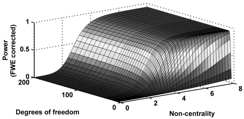
Once the local effect size is obtained, power is calculated at each voxel by the non-central RFT framework. However, this calculation involves numerical integrals and repeating the calculation at each voxel is impractical. To reduce the computational burden associated with generation of a power map, power is calculated for various combinations of nc and df beforehand, and a numerical interpolation is used on this power surface (see Figure 4) to approximate power. A power map is then obtained by finding power at each voxel for specific df. Similarly, a sample size map is obtained by finding df required to achieve a desired level of power.

Figure 4.

An example of a power surface. Power is described as a function of degrees of freedom and non-centrality.

Simulation-Based Validation

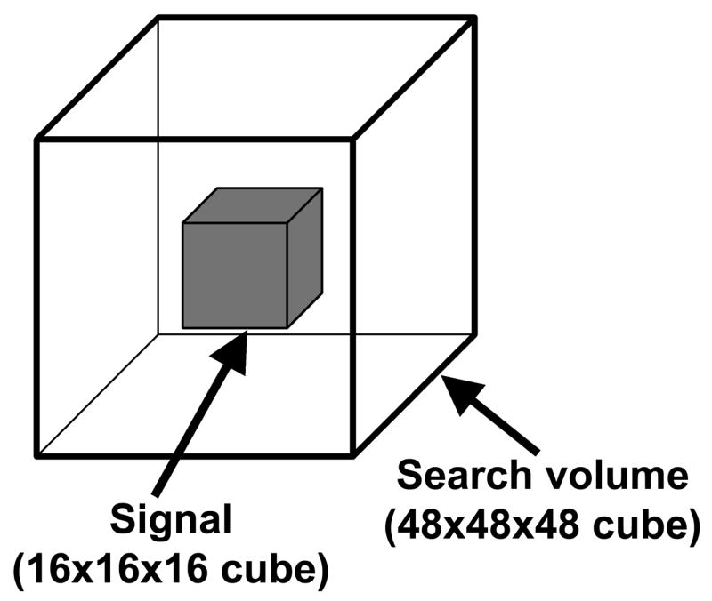
To evaluate the accuracy of power estimated from the non-central RFT framework, a simulation-based validation was carried out. In these simulations, we determined power to detect signals in a 16×16×16 voxel cube placed at the center of a 48×48×48 cube search volume (Figure 5). Since we are interested in the probability of detecting signals only within the smaller cube and not for the entire search volume, non-central random images were generated only for the smaller cube in the simulations. For each realization, a non-central T- or F-random image was produced by generating a number of independent smooth Gaussian random fields (Hayasaka and Nichols 2003; Nichols and Hayasaka 2003) and then calculating the non-central images from (1) or (2), respectively. Table 1 shows the settings for the simulations. During 1,000 iterations for each setting, the observed power was recorded as the probability that the maximum of the statistic image within the smaller cube exceeds the FWE-corrected threshold of p<0.05. The resulting observed power was compared to that of the non-central RFT framework.

Figure 5.

A schematic of the signal generated in the simulation. The signal (16×16×16 voxel cube) is located at the center of the search volume (48×48×48 voxel cube).

Table 1.

Simulation settings

	Non-central T simulation	Non-central F simulation
Smoothness (FWHM in voxels)	6, 9, 12, 15	6, 9, 12, 15
Degrees of freedom	6–20	Numerator: 2 (fixed) Denominator: 8–20
Effect size	0.75, 1.0, 1.5 (Cohen’s d)	0.75, 1.0, 1.5 (Cohen’s f)
Number of iterations	1,000 in each setting	1,000 in each setting

The simulations were carried out in MATLAB 6.5 (MathWorks Inc.; Natick, MA, USA) on a single processor on a Linux workstation with a Dual AMD Opteron 256 processor (3GHz) and 4GB of RAM.

Application

To demonstrate the use of the non-central RFT framework, we applied it to a BOLD fMRI data set from an auditory experiment in our laboratory. The data were obtained from 41 subjects (age=18–64, M/F=17/24) undergoing two runs of an auditory experiment. In each run, each subject was presented with alternating white noise and silence in a block design. During the experiment, a series of images were acquired with a gradient echo EPI (echo-planar imaging) sequence on a 1.5-T GE twin-speed LX scanner with a birdcage head coil (GE Medical Systems; Milwaukee, WI, USA). The parameters for the EPI images were: 24 cm field of view, 64×64 acquisition matrix, 28 slices with 5 mm thickness with no gap, TR/TE=2500/40 ms, in-plane resolution 3.75×3.75 mm, frequency direction anterior to posterior. Acquired functional images were spatially realigned, normalized to the Montreal Neurological Institute (MNI) space, smoothed using an 8×8×10 mm FWHM Gaussian kernel, and re-sampled to 2×2×2 mm voxels.

A multiple regression analysis was performed for each run with a box-car design convolved with the hemodynamic response function and an explicitly modeled baseline condition (rest block). Two paradigm runs for each subject were combined using a fixed-effect analysis, resulting in one contrast image per subject representing the mean activation associated with the auditory stimulus relative to baseline. All the preprocessing and the first-level analysis were done using our in-house automated program based on SPM99.

From the 41 contrast images, 5 were randomly chosen to form a mock pilot data set to estimate the effect size for planning future studies. On this mock pilot data, a one-sample T-test was performed with SPM2 to generate a T-statistic image (df=4) summarizing activations associated with the auditory stimulus. Since a simple auditory stimulus was used in the experiment, activations were expected in the bilateral primary auditory cortices (BA41, 42). To estimate the strength of activations in these areas, mean T-scores were calculated for left, right and both auditory cortices by the WFU PickAtlas toolbox (Maldjian, et al. 2004; Maldjian, et al. 2003) with a dilation factor of 3. A binary mask image was also produced for each of these areas, and RESEL counts were calculated to determine the topological characteristics for power calculation with (5). The effect size (Cohen’s d) was estimated based on the mean T-scores. Table 2 shows the RESEL counts, mean T-score, and effect size for each of these areas of anticipated signals. Power to detect activations (FWE-corrected) in these areas was calculated for various df to generate power curves. Moreover, a power map and a sample size map were also generated based on the same mock pilot data.

Table 2.

The RESEL counts, mean T-score, and effect sizes for different areas of anticipated signals.

Areas	RESEL counts				Mean T-score	Effect size (Cohen’s d)
	μ0	μ1	μ2	μ3
Entire brain	1	40.1	502.8	2317.8
Auditory cortices
Left	1	9.6	36.0	54.2	2.58	1.15
Right	1	9.6	36.1	54.9	2.22	0.99
Left or right	2	19.3	72.1	109.2	2.40	1.07

Results

Simulation

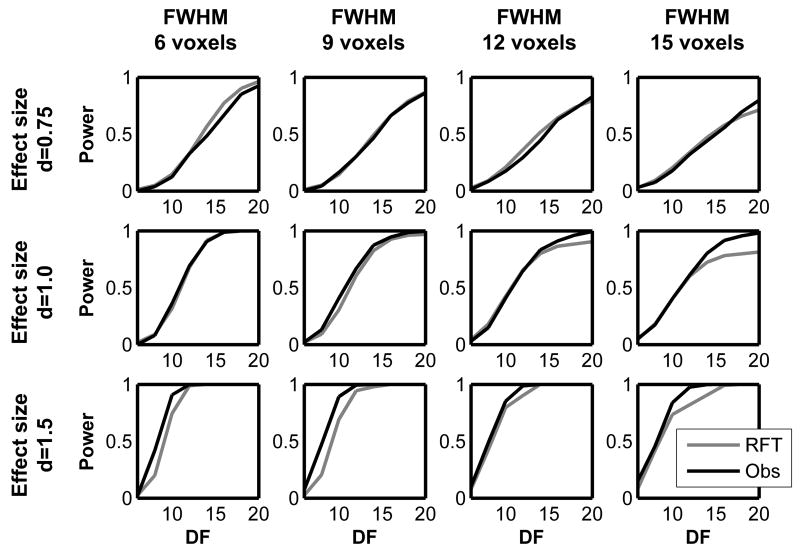
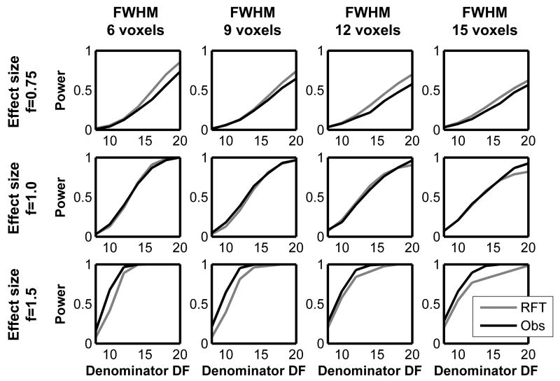
The simulation results are shown in Figures 6 and 7. Figure 6 displays the observed and RFT-based power from the non-central T-image simulation plotted for different effect sizes and smoothness. As it can be seen from the plots, the non-central RFT framework can estimate power accurately. Figure 7 displays the observed and RFT-based power from the non-central F-image simulation plotted for different effect sizes and smoothness. In the non-central F-image simulation, the RFT-based power seems to deviate from the observed power slightly more compared to the non-central T simulation, as seen in terms of the RMSE (root mean squared error) in Table 3. However, the RFT-based power still adequately approximates power. These results indicate our non-central RFT framework can be used to model power for known signals.

Figure 6.

The results from the non-central T simulation. The estimated power based on non-central RFT and the observed power are plotted against df for different smoothness and effect sizes.

Figure 7.

The results from the non-central F simulation. The estimated power based on non-central RFT and the observed power are plotted against denominator df for different smoothness and effect sizes. The numerator df is fixed (=2).

Table 3.

The RMSE (root mean square error) of the estimated power

Simulation	Effect size	FWHM
		6	9	12	15
Non-central T	d=0.75	0.05	0.01	0.04	0.04
	d=1.00	0.02	0.05	0.05	0.10
	d=1.50	0.10	0.12	0.04	0.08
Non-central F	f=0.75	0.08	0.05	0.08	0.05
	f=1.00	0.02	0.03	0.03	0.05
	f=1.50	0.11	0.12	0.06	0.11

The estimated power compared to the observed power for different settings of the non-central T- and F-image simulations.

As mentioned in Introduction, since the non-central RFT framework is theory-based, it is considerably more efficient than simulation-based power calculation in terms of computation. Table 4 shows the amount of time required to generate power curves for the non-central RFT method and the observed power curve based on the simulation seen on the second row of Figure 6. Although the simulation-based observed power curves can be considered as the gold standard, generating these power curves requires a considerable amount of computing time. On the other hand, it requires only several seconds to produce the RFT-based power curves. These results show that, in a study planning process, the non-central RFT framework is more advantageous than a simulation-based approach in terms of time and computational resources.

Table 4.

Computation time for generating a power curve (hours)

	Smoothness FWHM
	6	9	12	15
Non-central RFT-based	0.0007	0.0007	0.0007	0.0007
Simulation-based	2.4	9.0	19.9	42.5

For the non-central T-image simulation with effect size d=1.0.

Power Curves

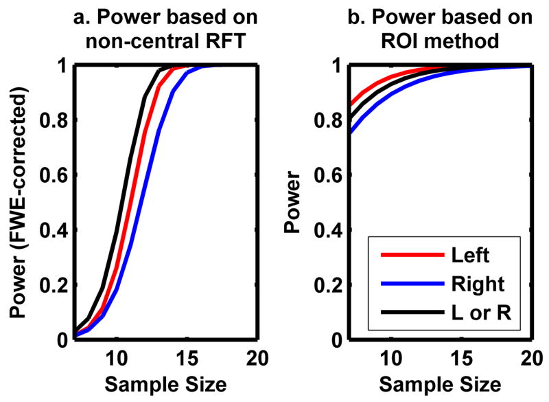
Figure 8a displays power curves for detecting signals in the left, right, and either auditory cortex calculated based on the non-central RFT framework obtained from the mock pilot analysis results. Since the effect size is slightly larger on the left auditory cortex, power to detect signal is slightly higher in the left auditory cortex than that on the right. Power is even higher when the signal to be detected is in either of the auditory cortices, since the total area is twice as large as the auditory cortex in either hemisphere alone.

Figure 8.

Power to detect signals in the left, right, and both auditory cortices was estimated for different degrees of freedom by the non-central RFT framework (a) and the conventional ROI-based power analysis (b).

For comparison purposes, we also calculated power using the single-outcome power analysis method (Cohen 1988) with the effect sizes calculated in the same ROIs (region of interest) listed in Table 2 (see Figure 8b). In this case, the effect size is the only factor determining power, thus power is expected to be higher in the left auditory cortex alone than for both auditory cortices together. This is somewhat counterintuitive because including the right auditory cortex actually decreases power. The sample size determined by the ROI-based power was somewhat smaller than that of the non-central RFT and this could lead to an underpowered study. For example, to detect signals in either of the auditory cortices with at least 80% power, the non-central RFT estimated that at least 12 subjects would be required while the ROI method estimated that only 7 subjects would be needed.

Power and Sample Size Maps

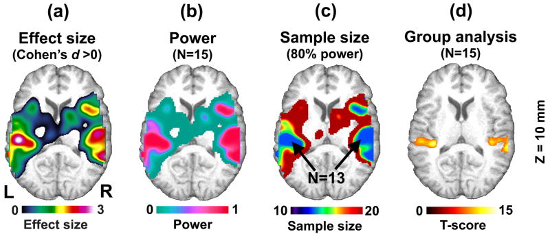
In our mock pilot data analysis using 5 subjects, we were not able to detect any activation with the FWE-corrected threshold of p<0.05 due to small df (=4). However, we were able to use the T-statistic image from the mock pilot analysis to generate a power map. Figure 9a shows the effect size map obtained based on the mock pilot analysis (Cohen’s d >0), and Figure 9b shows the power map showing the estimated power if 15 subjects were included in this analysis. In the power map, relatively high power can be seen in the bilateral auditory cortices. We also generated a sample size map based on the mock pilot analysis (Figure 9c), and found that approximately 13 subjects would be required to detect signals in the auditory cortices with 80% power. To confirm this finding, we randomly selected a set of 15 contrast images from the remaining 36 contrast images in the original data set and performed the same analysis to detect activations (Figure 9d). From this follow-up analysis with 15 subjects, we detected activations in the bilateral auditory cortices as anticipated with the FWE-corrected threshold of p<0.05.

Figure 9.

From the mock pilot analysis results, an effect size map was generated (Cohen’s d >0) (a). Based on this effect size, a power map was generated for N=15 subjects (b). The corresponding sample size map was also generated to determine the number of subjects required to detect signals with 80% power (c). Activations in the bilateral auditory cortices were found in the follow-up analysis with 15 randomly selected subjects from the fMRI data pool (d). The maps (b)-(d) are corrected for multiple comparisons (p<0.05, FWE corrected at voxel-level).

Discussion

In this paper, we presented a theory-based framework for power calculation in neuroimaging data analysis. The framework is an extension of RFT to non-central T- and F-random fields. We demonstrated in our simulations that this non-central RFT framework was able to approximate power quite accurately for non-central T- and F-random fields with known signals. We also demonstrated an application of this method in a simple fMRI data analysis. We were able to generate power curves for explicitly known areas of anticipated signals. We were also able to visualize locally varying sensitivity in the form of power and sample size maps.

The non-central RFT framework offers several advantages over the existing power calculation methods for neuroimaging data analysis. Our method is able to calculate power corrected for multiple comparisons among correlated voxels. Moreover, since our method calculates power to detect signals not for a particular voxel but for a collection of voxels, the 3D nature of signals is more appropriately modeled than methods focused on a specific voxel or ROI. Our method is implemented by a parametric model; hence power can be calculated for different parameters and settings without a large computational burden. As a result, power curves can be easily generated when the alternative hypothesis can be explicitly specified as areas of anticipated signals. Even when there are no explicit areas of anticipated signals, visualization of varying sensitivity is possible via power and sample size maps. Such power curves and power maps can be generated from a pilot data set with a limited number of subjects, as demonstrated.

As an alternative to our approach, we can also consider the RFT-based approach by Friston et al. (1994) mentioned in Introduction. In this simpler approach, signals are modeled as a Gaussian white noise process with larger variance centered at zero, and added to the background noise process. This inflated variance method can calculate power by simply adjusting the critical threshold u_c and the image smoothness FWHM h. For example, power for a T-test can be calculated as

$$\lambda =1-exp\left\{\sum _{i=0}^3{\mu }_i^{\ast }(B){\rho }_i(u_c^{\ast })\right\}$$

with the adjusted critical threshold $u_c^{\ast }$

$$u_c^{\ast }=\frac{u_c}{\sqrt{1+d^2}}$$

and with the RESEL count ${\mu }_i^{\ast }$ based on the adjusted FWHM h*

$$h^{\ast }=h\sqrt{(1+d^2)/\left(1+\frac{d^2}{2}\right)}.$$

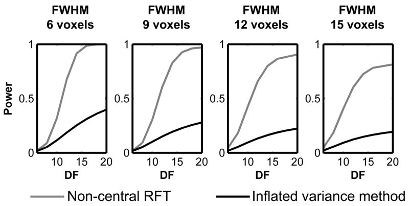
It should be noted that, power estimated by this inflated variance method could be considerably smaller compared to that estimated by the non-central RFT framework. Figure 10 shows an example of such a discrepancy in power by comparing estimated power between the two methods for detecting the signal described in Figure 5.

Figure 10.

Estimated power for a T-test to detect the signal described in Figure 5 with effect size d=1.0 and various image smoothness settings. Power was estimated by the non-central RFT framework (gray lines) and the inflated variance method (black lines). The estimated power is consistently smaller for the inflated variance method compared to that from the non-central RFT framework.

Although the non-central RFT framework can overcome problems mentioned in Introduction, there are some challenges and limitations associated with RFT-based methods to be considered. In order for RFT to work properly, various assumptions need to be met, including smooth random fields, sufficiently large search volume relative to the FWHM of images, and uniform smoothness within images (Hayasaka and Nichols 2003; Nichols and Hayasaka 2003; Worsley, et al. 1992). As for uniform smoothness, there are some approaches to overcome the violation in this assumption (Hayasaka, et al. 2004; Worsley, et al. 1999). However, such approaches require estimating smoothness at each voxel and introduce great variability in statistical inference (Hayasaka, et al. 2004). Thus such corrections for non-uniform smoothness may not be appropriate for a typical pilot data with a limited number of scans. Another shortcoming is that RFT-based methods can model only the extreme tail of the distribution of the maximum (Worsley 1994). This is less problematic in statistical inference, but in power analysis, power may need to be calculated at a somewhat distant location from the extreme tail in some situations. For such situations, we introduced ad-hoc adjustments such as the df offset and the linear extrapolation of power. However, more theoretical solutions are desired for these situations.

There are some possible extensions from the non-central RFT framework. Since the distribution of the cluster extent can be approximated theoretically for central random fields (Cao 1999; Friston, et al. 1994), such theoretical framework may also be extended to non-central random fields. This may be of interest to many investigators since inference based on the cluster extent is known to be more powerful than the one based on voxel intensity (Friston, et al. 1996). Another possible extension is to calculate FWE-corrected power using a Bonferroni correction (Zarahn and Slifstein 2001). A Bonferroni-based approach may be appropriate for neuroimaging data with reduced smoothness where RFT-based methods are conservative (Nichols and Hayasaka 2003; Worsley 2005).

The non-central RFT framework can also be extended to situations where investigators are interested in detecting signals in multiple areas within the brain simultaneously. In such a case, different areas of interest can be treated as patches of independent non-central random fields, each having different effect size. Unless these patches are in close proximity to each other, independence among them is a reasonable assumption. Then a power curve can be calculated for each of these areas separately, and multiplying the resulting power curves from all the areas can yield the desired power estimate. For example, in our earlier example of power curves for signals in the auditory cortices (Figure 8), we can also calculate power to detect signals in both left and right auditory cortices occurring simultaneously by multiplying the power curves from both cortices. For even more complex scenarios, such as detecting signals in a certain proportion of areas of interest, power can be easily calculated by simple probability operations under the assumption of independent patches of random fields.

In conclusion, the non-central RFT framework provides neuroimaging investigators a simple and quick way to calculate power for their studies. Even from a pilot data set with a small sample size, power and sample size can be easily estimated for future study planning. Additionally, the results from power calculation can be readily interpreted visually in the form of power and sample size maps. The methodology presented in this paper could greatly improve the planning process of neuroimaging studies.

Appendix A: RESEL Densities for Non-central Random Fields

We list the RESEL densities for non-central T- and F-random fields below. Details on the derivation of these results are found in Hayasaka (2007). In brief, for a D-dimensional random field X, the i-dimensional (i ≤ D) RESEL density ρ_i(u) is given by

$${\rho }_i(u)=\left\{{(-1)}^{i-1}E\left[{\dot{X}}^{(i)+}det\left({\ddot{X}}_{i-1}\right)\mid X=u,{\dot{X}}_{i-1}=0\right]{\theta }_{i-1}\left({\dot{X}}_{i-1}=0\right)\right\}\left(\frac{\sqrt{det(\mathrm{\Lambda })}}{{(4log2)}^{i/2}}\right)$$

where Ẋ_i−1 and Ẍ_i−1 denote the first i −1 and (i − 1) × (i− 1) elements of the first and second derivatives of X respectively, Ẋ⁽ⁱ⁾⁺ denotes the positive portion of the i-th element of Ẋ, and Λ denotes the covariance matrix of the gradient of the Gaussian random field Z in (1) and (2) (Worsley 1994). The probability density function of Ẋ_i−1 is denoted by θ_i−1.

Alternatively, RESEL densities for non-central random fields can be found by the Gaussian Kinematic Formula (Taylor 2006) without finding the derivatives. This can be done because the density of a non-central random variable can be expressed as a sum of central random variables with different df. Taylor (2006) demonstrated this on a non-central χ² random field. This can be extended to non-central T- and F-random fields.

Non-Central T-Random Field

The RESEL densities for a non-central T-random field with df=m and nc=δ at the threshold u are given as

$${{\rho }_0}^{\prime }(u;\delta )={\int }_u^{\infty }{f}_S(y)dy$$

$${{\rho }_1}^{\prime }(u;\delta )={\left(\frac{4log2}{2\pi }\right)}^{\frac{1}{2}}\sqrt{m}\left(1+\frac{u^2}{m}\right)E\left[W^{-\frac{1}{2}}\right]f_S(u)$$

$${{\rho }_2}^{\prime }(u;\delta )=\frac{4log2}{2\pi }\sqrt{m}\left(1+\frac{u^2}{m}\right)\left\{(m-1){\left(\frac{u^2}{m}\right)}^{\frac{1}{2}}E\left[W^{-1}\right]-{\left(1+\frac{u^2}{m}\right)}^{-\frac{1}{2}}E\left[W^{-\frac{1}{2}}\right]\delta \right\}{f}_S(u)$$

$$\begin{array}{l}{{\rho }_3}^{\prime }(u;\delta )={\left(\frac{4log2}{2\pi }\right)}^{\frac{3}{2}}\sqrt{m}\left(1+\frac{u^2}{m}\right)\{(m-1)(m-2)\left(\frac{u^2}{m}\right)E\left[W^{-\frac{3}{2}}\right]\\ -2(m-1){\left(\frac{u^2}{m}\right)}^{\frac{1}{2}}{\left(1+\frac{u^2}{m}\right)}^{-\frac{1}{2}}E\left[W^{-1}\right]\delta +{\left(1+\frac{u^2}{m}\right)}^{-1}E\left[W^{-\frac{1}{2}}\right]{\delta }^2-E\left[W^{-\frac{1}{2}}\right]\}{f}_S(u)\end{array}$$

where f_S is the probability density function of a non-central T-random variable with df=m and nc= δ, and W is a non-central chi-square random variable with df=m+1 and nc=δ².

The density function f_S (Lehmann 1986) is given by

$$f_S(u)=\frac{1}{2^{\frac{m-1}{2}}\mathrm{\Gamma }\left(\frac{m}{2}\right)\sqrt{m\pi }}{\int }_0^{\infty }{y}^{\frac{m-1}{2}}exp\left(-\frac{y}{2}\right)exp\left(-\frac{1}{2}{\left\{u\sqrt{\frac{y}{m}}-\delta \right\}}^2\right)dy.$$

The expectation W^b (Johnson, et al. 1995) of a non-central chi-square random variable W with df=ν and nc=ϕ is given by

$$E\left[W^b\right]=2^b\mathrm{\Gamma }\left(b+\frac{\nu }{2}\right)\sum _{j=0}^{\infty }\frac{\mathrm{\Gamma }(b+1)}{\mathrm{\Gamma }(j+1)\mathrm{\Gamma }(b-j+1)}{\left(\frac{\varphi }{2}\right)}^j\frac{1}{\mathrm{\Gamma }\left(j+\frac{\nu }{2}\right)}.$$

Non-Central F-Random Field

The RESEL densities for a non-central F-random field with df=m,n and nc=η at the threshold u are given as

$${{\rho }_0}^{\prime }(u;\eta )={\int }_u^{\infty }{f}_G(y)dy$$

$${{\rho }_1}^{\prime }(u;\eta )={\left(\frac{4log2}{2\pi }\right)}^{\frac{1}{2}}2\left(1+\frac{m}{n}u\right){\left(\frac{m}{n}u\right)}^{\frac{1}{2}}E\left[W^{-\frac{1}{2}}\right]\left(\frac{n}{m}\right)f_G(u)$$

$${{\rho }_2}^{\prime }(u;\eta )=\frac{4log2}{2\pi }2\left(1+\frac{m}{n}u\right)E\left[W^{-1}\right]\left\{(n-1)\left(\frac{m}{n}u\right)-(m-1+\eta )\right\}\left(\frac{n}{m}\right)f_G(u)$$

$$\begin{array}{l}{{\rho }_3}^{\prime }(u;\eta )={\left(\frac{4log2}{2\pi }\right)}^{\frac{3}{2}}2\left(1+\frac{m}{n}u\right){\left(\frac{m}{n}u\right)}^{-\frac{1}{2}}\{E\left[W^{-\frac{3}{2}}\right]\\ \left((m-1)(m-2)-2(n-1)(m-1+\eta )\left(\frac{m}{n}u\right)+(n-1)(n-2){\left(\frac{m}{n}u\right)}^2+(2m-1+\eta )\eta \right)\\ -\left(\frac{m}{n}u\right)E\left[W^{-\frac{1}{2}}\right]\}\left(\frac{n}{m}\right)f_G(u)\end{array}$$

where f_G is the probability density function of a non-central F-random variable with df=m,n and nc=η, and W is a non-central chi-square random variable with df=m+n and nc=η. The density function f_G (Johnson, et al. 1995) is given by

$$f_G(u)=e^{-\frac{\eta }{2}}\frac{m^{\frac{m}{2}}{n}^{\frac{n}{2}}}{\beta \left(\frac{m}{2},\frac{n}{2}\right)}\frac{u^{\frac{m}{2}-1}}{{(n+mu)}^{\frac{m+n}{2}}}\sum _{j=0}^{\infty }{\left(\frac{\eta mu}{2(n+mu)}\right)}^j\frac{\mathrm{\Gamma }\left(\frac{m+n}{2}+j\right)}{j!\mathrm{\Gamma }\left(\frac{m+n}{2}\right)}\frac{\mathrm{\Gamma }\left(\frac{m}{2}\right)}{\mathrm{\Gamma }\left(\frac{m}{2}+j\right)}$$

where β is the beta function.

References

- Adler RJ. The Geometry of Random Fields. New York: Wiley; 1980. [Google Scholar]
- Bullmore ET, Suckling J, Overmeyer S, Rabe-Hesketh S, Taylor E, Brammer MJ. Global, voxel, and cluster tests, by theory and permutation, for a difference between two groups of structural MR images of the brain. IEEE Trans Med Imaging. 1999;18:32–42. doi: 10.1109/42.750253. [DOI] [PubMed] [Google Scholar]
- Cao J. The Size of the Connected Components of Excursion Sets of Chi-squared, t and F Fields. Advances in Applied Probability. 1999;31:579–595. [Google Scholar]
- Cao J, Worsley KJ. The Geometry of Correlation Fields with an Application to Functional Connectivity of the Brain. Annals of Applied Probability. 1999;9:1021–1057. [Google Scholar]
- Cao J, Worsley KJ. Applications of Random Fields in Human Brain Mapping. In: Moore M, editor. Spatial Statistics: Methogological Aspects and Applications. Springer; 2001. pp. 169–182. [Google Scholar]
- Cohen J. Statistical Power Analysis for the Behavioral Sciences. Hillsdale, NJ: Lawrence Erlbaum Associates; 1988. [Google Scholar]
- Desmond JE, Glover GH. Estimating sample size in functional MRI (fMRI) neuroimaging studies: statistical power analyses. J Neurosci Methods. 2002;118:115–28. doi: 10.1016/s0165-0270(02)00121-8. [DOI] [PubMed] [Google Scholar]
- Friston KJ, Holmes A, Poline JB, Price CJ, Frith CD. Detecting activations in PET and fMRI: levels of inference and power. Neuroimage. 1996;4:223–35. doi: 10.1006/nimg.1996.0074. [DOI] [PubMed] [Google Scholar]
- Friston KJ, Holmes AP, Worsley KJ. How many subjects constitute a study? Neuroimage. 1999;10:1–5. doi: 10.1006/nimg.1999.0439. [DOI] [PubMed] [Google Scholar]
- Friston KJ, Worsley KJ, Frackowiak RSJ, Mazziotta JC, Evans AC. Assessing the significance of focal activations using their spatial extent. Human Brain Mapping. 1994;1:210–220. doi: 10.1002/hbm.460010306. [DOI] [PubMed] [Google Scholar]
- Hayasaka S. Derivation of the Euler Characteristic Densities of Non-Central T- and F-Random Fields. Technical Bulletin, ANSIR Laboratory. 2007 http://www.fmri.wfubmc.edu/
- Hayasaka S, Nichols TE. Validating cluster size inference: random field and permutation methods. Neuroimage. 2003;20:2343–56. doi: 10.1016/j.neuroimage.2003.08.003. [DOI] [PubMed] [Google Scholar]
- Hayasaka S, Phan KL, Liberzon I, Worsley KJ, Nichols TE. Nonstationary cluster-size inference with random field and permutation methods. Neuroimage. 2004;22:676–87. doi: 10.1016/j.neuroimage.2004.01.041. [DOI] [PubMed] [Google Scholar]
- Holmes AP, Blair RC, Watson JD, Ford I. Nonparametric analysis of statistic images from functional mapping experiments. J Cereb Blood Flow Metab. 1996;16:7–22. doi: 10.1097/00004647-199601000-00002. [DOI] [PubMed] [Google Scholar]
- Johnson NL, Kotz S, Balakrishnan N. Continuous Univariate Distributions. New York: John Wiley & Sons, Inc; 1995. [Google Scholar]
- Lehmann EL. Testing Statistical Hypotheses. New York: Springer-Verlag; 1986. [Google Scholar]
- Maldjian JA, Laurienti PJ, Burdette JH. Precentral gyrus discrepancy in electronic versions of the Talairach atlas. Neuroimage. 2004;21:450–5. doi: 10.1016/j.neuroimage.2003.09.032. [DOI] [PubMed] [Google Scholar]
- Maldjian JA, Laurienti PJ, Kraft RA, Burdette JH. An automated method for neuroanatomic and cytoarchitectonic atlas-based interrogation of fMRI data sets. Neuroimage. 2003;19:1233–9. doi: 10.1016/s1053-8119(03)00169-1. [DOI] [PubMed] [Google Scholar]
- Murphy K, Garavan H. An empirical investigation into the number of subjects required for an event-related fMRI study. Neuroimage. 2004;22:879–85. doi: 10.1016/j.neuroimage.2004.02.005. [DOI] [PubMed] [Google Scholar]
- Nichols T, Hayasaka S. Controlling the familywise error rate in functional neuroimaging: a comparative review. Stat Methods Med Res. 2003;12:419–46. doi: 10.1191/0962280203sm341ra. [DOI] [PubMed] [Google Scholar]
- Nichols TE, Holmes AP. Nonparametric permutation tests for functional neuroimaging: a primer with examples. Hum Brain Mapp. 2002;15:1–25. doi: 10.1002/hbm.1058. [DOI] [PMC free article] [PubMed] [Google Scholar]
- Siegmund DO, Worsley KJ. Testing for a Signal with Unknown Location and Scale in a Stationary Gaussian Random Field. The Annals of Statistics. 1995;23:608–639. [Google Scholar]
- Taylor JE. A Gaussian Kinematic Formula. The Annals of Probability. 2006;34:122–158. [Google Scholar]
- Van Horn JD, Ellmore TM, Esposito G, Berman KF. Mapping voxel-based statistical power on parametric images. Neuroimage. 1998;7:97–107. doi: 10.1006/nimg.1997.0317. [DOI] [PubMed] [Google Scholar]
- Worsley KJ. Local Maxima and the Expected Euler Characteristic of Excursion Sets of chi-squared, F and t Fields. Advances in Applied Probability. 1994;26:13–42. [Google Scholar]
- Worsley KJ. The geometry of random images. Chance. 1996;9:27–40. [Google Scholar]
- Worsley KJ. An improved theoretical P value for SPMs based on discrete local maxima. Neuroimage. 2005;28:1056–62. doi: 10.1016/j.neuroimage.2005.06.053. [DOI] [PubMed] [Google Scholar]
- Worsley KJ, Andermann M, Koulis T, MacDonald D, Evans AC. Detecting changes in nonisotropic images. Hum Brain Mapp. 1999;8:98–101. doi: 10.1002/(SICI)1097-0193(1999)8:2/3<98::AID-HBM5>3.0.CO;2-F. [DOI] [PMC free article] [PubMed] [Google Scholar]
- Worsley KJ, Evans AC, Marrett S, Neelin P. A three-dimensional statistical analysis for CBF activation studies in human brain. J Cereb Blood Flow Metab. 1992;12:900–18. doi: 10.1038/jcbfm.1992.127. [DOI] [PubMed] [Google Scholar]
- Worsley KJ, Marrett S, Neelin P, Evans AC. Searching scale space for activation in PET images. Human Brain Mapping. 1996a;4:74–90. doi: 10.1002/(SICI)1097-0193(1996)4:1<74::AID-HBM5>3.0.CO;2-M. [DOI] [PubMed] [Google Scholar]
- Worsley KJ, Marrett S, Neelin P, Vandal AC, Friston KJ, Evans AC. A unified statistical approach for determining significant signals in images of cerebral activations. Human Brain Mapping. 1996b;4:58–73. doi: 10.1002/(SICI)1097-0193(1996)4:1<58::AID-HBM4>3.0.CO;2-O. [DOI] [PubMed] [Google Scholar]
- Zarahn E, Slifstein M. A reference effect approach for power analysis in fMRI. Neuroimage. 2001;14:768–79. doi: 10.1006/nimg.2001.0852. [DOI] [PubMed] [Google Scholar]