Efficient Calculation of Exact Mass Isotopic Distributions

Abstract

This paper presents a new method for efficiently calculating the exact masses in an isotopic distribution using a dynamic programming approach. The resulting program, isoDalton, can generate extremely high isotopic resolutions as demonstrated by a FWHM resolution of 2×10¹¹. This resolution allows very fine mass structures in isotopic distributions to be seen, even for large molecules. Since the number of exact masses grows exponentially with molecular size, only the most probable exact masses are kept, the number of which is user specified.

Introduction

For most practical applications, computing the very fine isotopic structure is unnecessary as it is beyond the resolution of today’s mass spectrometers. However, for theoretical considerations, it is useful to have a method that can calculate the exact mass distributions of these fine structure clusters, which could prove useful as the resolution of mass spectrometers improves. One of the challenges in calculating distributions is maintaining a very high resolution around isotope peaks and yet being computationally efficient.

A number of methods [1–9] have been employed to elucidate the fine isotopic structure. The majority are polynomial based methods that rely on pruning to reduce the complexity to a more manageable size. The pruning strategies typically use a threshold to eliminate permutations whose contribution falls below some preset value. This creates errors in the isotopic distribution profile since a significant number of terms are eliminated.

Rockwood et. al [8–9] uses a Fourier transform method to zoom in and achieve ultrahigh resolution around a single mass peak. As with any Fourier analysis method, care must be taken to choose an appropriate window function. The windowing will cause the underlying Dirac delta functions representing fine isotopic masses to be convolved together if they are closer together than the width of the analysis window.

A new method based on dynamic programming [10] is presented that can efficiently calculate isotopic distributions. In principle, the resolution is infinite, since there is no restriction on how close in mass the states can be to each other. In practice, the resolution seen depends on machine precision and the probability of the mass states.

Low probability states that are very close to other more probable states may either be eliminated or merged, depending on the state reduction strategy employed.

This method can operate like a polynomial pruning method if low probability states are eliminated. If neighboring states are merged instead, it can operate more like the Fourier transform method. In the Fourier transform method, all peaks under the window contribute whereas the merging in the dynamic programming case is local.

The implementation of the algorithm is a program called isoDalton that has been written in MATLAB [12] and is freely available under the GNU Lesser General Public License [13], which allows use in both proprietary and free programs. The program includes all the isotopes of all the elements with the standard isotopic compositions [14]. Custom isotopic compositions can be easily added.

Algorithm Description

Calculating ion distributions for large molecules require expanding the polynomial of the form

$${(E_1^1+E_2^1+\cdots +E_{I_1}^1)}^{N_1}{(E_1^2+E_2^2+\cdots +E_{I_2}^2)}^{N_2}{(E_1^3+E_2^3+\cdots +E_{I_3}^3)}^{N_3}\dots$$ (1)

where $E_j^i$ represents the j^th isotope of the i^th element in the molecule. The N_i superscript outside the parenthesis represents the number of atoms of the i^th element [4]. This will generate a combinatorial explosion in the number of terms for large molecules. The number of coefficients for the multinomial ${(E_1^i+E_2^i+\cdots +E_{I_i}^i)}^{N_i}$ representing the i^th element with N_i atoms and I_i isotopes is given by [15]:

$$C_{I_i}^{N_i}=\frac{(N_i+I_i-1)!}{N_i!(I_i-1)!}$$ (2)

and the coefficients of the multinomial are given by:

$${(E_1^i+E_2^i+\cdots +E_{I_i}^i)}^{N_i}=\sum _{M_1+M_2+\cdots +M_{I_i}=N_i}\frac{N_i!}{M_1!M_2!\cdots M_{I_i}!}{E}_1^{i{M}_1}{E}_1^{i{M}_2}\cdots E_1^{i^M{I}_i}$$ (3)

The total number of terms T in the expanded polynomial of equation 1 is the number of terms in the product of the elemental multinomial coefficients and is given by:

$$T=C_{I_1}^{N_1}{C}_{I_2}^{N_2}{C}_{I_3}^{N_3}\cdots$$ (4)

which gives the number of possible masses in the isotopic fine structure.

For bovine insulin C₂₅₄H₃₇₇N₆₅O₇₅S₆ the number of possible terms is 1.56 × 10¹², which clearly precludes any brute force attack. In practice, one only needs a fraction of the terms since most of the terms are extremely unlikely. The least probable term is ¹³C₂₅₄²H₃₇₇¹⁵N₆₅¹⁷O₇₅³⁵S₆ that has a probability of 0.2610×10⁻²⁴²² of occurring. In fact, the top 1,000 terms represents 99.96 % of the cumulative probability distribution.

An efficient method based on dynamic programming can be used to calculate the overall distribution of possible molecular weights given the isotopic distribution for each element. To apply dynamic programming, we first frame this calculation in the context of a Markov process {X_t}_t∈T operating on a discrete state space S. The state transition probabilities are given by:

$$p_{ij}=P(X_{n+1}=j\mid X_n=i),n\ge 0,i,j\in S$$ (5)

This gives the probability of arriving at state S_j at step n+1, given that it was in state S_i at step n. The state transition probabilities are required to have the following properties:

$$\begin{array}{l}{p}_{ij}\ge 0\\ \sum _{j=1}^J{p}_{ij}=1,\forall i,\hspace{0.17em}j=1,\dots ,J.\end{array}$$ (6)

The initial state probabilities are given by:

$${\pi }_i(0)=P(X_0=i),i\in S$$ (7)

The efficient way to calculate the probability of being in state S_j at step n+1 is to use a forward trellis algorithm [16]. An illustration of this computation can be seen in figure 1.

Figure 1.

Trellis for efficiently computing state probabilities.

The state probabilities for step n+1 are calculated by

$${\alpha }_{S_j}(n+1)=\sum _{i=1}^{N(n)}{\alpha }_{S_i}(n)p_{ij}$$ (8)

where 1 ≤ j ≤ N(n+1),1 ≤ n ≤ T − 1. N(n) implies that the number of states is a function of step n.

The trellis algorithm gains its efficiency by collapsing the possible paths that can lead to a particular state. Only the state probabilities at step n along with the transition probabilities are used to calculate the state probabilities for the next step. This is known as a first order markov model or chain [17].

In the context of calculating the isotope distribution, the states are the set of unique molecular masses that can exist at each step. At each step, all isotopes of one atom of a particular element are added, i.e. ${(E_1^i+E_2^i+\cdots +E_{I_1}^i)}^1$. This means that the state transition probabilities are non-stationary since they depend on the isotope distribution of the particular element being added. The Markov chain can be thought of as the sequence of adding elements with all associated isotopes at each step. The length of the chain is the number of elements in the molecule.

The number of states at each step is also non-stationary since particular combinations of isotopes lead to unique masses. The states at step n+1 is the set of unique masses computed by adding the mass of any state at step n with any isotope of the element being added. The probabilities of these states are given in equation 8. These states are then either pruned or combined to reduce computational complexity and this process is call state reduction.

State Reduction

Most Probable Exact Masses

Keeping the distribution of all exact masses becomes impractical for all but the smallest molecules. If one is interested in the exact masses of the most probable isotope mass combinations, as is typically the case, then the states with lowest probabilities are eliminated. This is done by computing all states for step n+1, sorting these states based on probabilities, and then keeping only the top N_max most probable states where N_max is user specified. Once all the elements have been added at the last step, isoDalton returns the exact masses of the N_max most probable isotopic mass combinations. The “true” probabilities of these exact masses are only approximations since eliminating states prunes potential path combinations that affect probability values. Increasing N_max will reduced this error.

Exact Probability Distribution

If one is interested in seeing the overall probability distribution of near integer separated values, then close mass values can be combined as follows. Let M_old1 and M_old2 be the masses of states S_i and S_j that are the closest together in terms of mass values and let P_old1 and P_old2 be their respective probabilities. Then a new state is created that has mass and probability of:

$$M_{\mathit{new}}=(M_{\mathit{old}1}{P}_{\mathit{old}1}+M_{\mathit{old}2}{P}_{\mathit{old}2})/(P_{\mathit{old}1}+P_{\mathit{old}2})$$ (9)

$$P_{\mathit{new}}=P_{\mathit{old}1}+P_{\mathit{old}2}$$ (10)

For a particular step n, the states are combined in this fashion until there are N_max states. Combining states in this manner results in a probability distribution of N_max masses that are the center of masses of the isotopic fine structure exact masses. These are exact probabilities for these “center of mass” weights since they sum to 1 as expected of a probability distribution. However, the masses are not exact.

Results and Discussion

As an example, we find the complete molecular weight distribution of the amino acid Glycine, C₂H₅N₁O₂ (including the amino and carboxyl end groups). We view the Markov process as the sequence of adding the elements H, H, H, H, H, C, C, N, O, and O, where the order of elements is taken by starting with the element with the fewest number of isotopes. Starting with elements with fewest isotopes minimizes the growth in the number of states. The isotopes used in this example are the NIST values [14].

The initial state probability π(0) is simply the isotopic composition of hydrogen {0.999885, 0.000115} at states (masses) {1.0078250321, 2.0141017780}. To compute the new state probabilities, we add another hydrogen and compute the resulting states and probabilities of being in these states. The new states at step n+1 are all permutations of adding the molecular weights of the states at step n with all the isotopes of element Eⁱ. The atomic weights for all states at each step can be seen in figure 2. This was created by adding the Glycine elements H, H, H, H, H, C, C, N, O, O.

Figure 2.

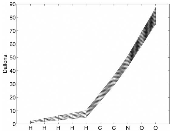
Trellis showing all mass states for Glycine C₂H₅N₁O₂.

A more abstract view of the trellis can be accomplished by finding at each step the state with the minimum atomic weight, and then subtracting this value from all states for this step. Figure 3 shows this abstracted view where the distances between states can be more clearly seen. The bottom row in the figure shows which element was added at each step. Above the trellis, the number of states is given that exist for each step. We start off with two states since Hydrogen has two isotopes and we end up with 216 states, or distinct atomic weights after adding all 10 elements. Many of the states are clustered together near unitary atomic weight increments. In practice, only the states at step n are kept since the state history is not needed and would only consume memory.

Figure 3.

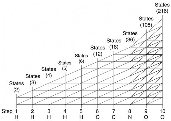
Abstract view of trellis formation for Glycine C₂H₅N₁O₂.

The complete molecular weight distribution of Glycine can be seen in figure 4. The distribution is plotted with two different scales. Positive values are the probabilities of isotopic masses where the scale is on the left upper side. Since most of the probabilities are very small, a log scale is plotted by taking the log10 of the probabilities. This results in negative numbers that are seen in the lower half of the plot with the scale on the right lower side. There are 216 unique mass values in this plot that are clustered near 13 integer values. There is a single dominant peak at mass 75.03 with probability 0.97. There are four mass values clustered at 76.03 and are shown in the inset plot. There is a very small single peak at mass 87.08 with probability 3.56×10⁻³² and can be seen clearly on the log10 scale with value −31.4484. The closest states occur at 81.05 with a separation of 7.21 × 10⁻⁵, which means a FWHM resolution of 1.12 × 10⁶ is needed to resolve these peaks.

Figure 4.

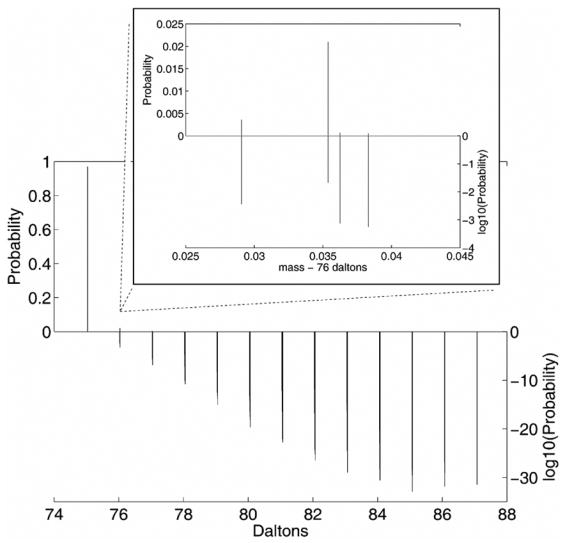
Complete isotopic distribution of Glycine C₂H₅N₁O₂. There are 216 unique masses of which the probabilities are shown on two scales. These two scales are the typical probability scale (upper left) and the log10 probability scale (lower right) that shows the improbable peaks (large negative log values). The inset plot shows 4 peaks that comprise the 76.03 dalton isotopic cluster.

For large molecules, keeping all unique states will cause the number of states to grow too large for memory and speed considerations. To keep the states small and still have a useful distribution, one can combine the states by adding clustered weights together. This is done by adding all the probabilities together in a cluster. In the Glycine example, this would reduce the number of final states from 216 to 13. As a result, one can trade off distribution precision for a reduction in computational complexity.

To show the program’s utility with large molecules, bovine insulin C₂₅₄H₃₇₇N₆₅O₇₅S₆ was chosen for comparison purposes with previous publications. Figure 5 shows the fine isotopic structure around the 5736.6 Da peak of protonated bovine insuline with a FWHM resolution of 2 × 10¹¹, which is a resolution of several orders of magnitude finer than previously shown. This distribution was calculated by keeping the top 100,000 most probable states, 416 of which are near the 5736.6 peak. The resolution is similar for the other isotopic clusters that range in mass from 5730.6 to 5759.7.

Figure 5.

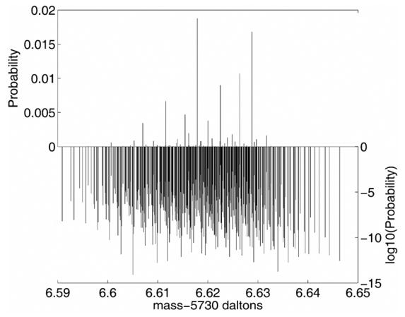
Isotopic fine structure of the 5736.6 peak of protonated Bovine Insulin C₂₅₄H₃₇₇N₆₅O₇₅S₆ shown with a FWHM resolution of 2 × 10¹¹. The distribution is plotted against two scales. The scale on the top left plots the probability of mass terms. However, most of the mass terms have very low probabilities and do not show up in the probability plot since they are essentially zero. To show these terms, a log10 scale is shown on the bottom right. Each mass term is shown in each scale, at the same mass location. There are 416 distinct mass terms in this cluster from an overall distribution of the 100,000 most probable mass states.

Run times

There is a tradeoff between execution speed and the FWHM resolution. Table 6 shows the tradeoff between the number of states and the run time for exact mass calculations. The time per state actually gets better with additional states due to a relatively fixed overhead of processing the state vectors in the program.

Conclusion

The paper presents a new method based on dynamic programming that can calculate the distribution of exact masses in an isotopic distribution. The resulting Matlab program isoDalton can be used to calculate the isotopic fine structure of large molecules with extremely high resolution. This is done by keeping only the most probable states representing exact masses. The program can also calculate isotopic distributions with a true probability profile at the expense of knowing exact masses by merging very close mass states.

Table 1.

Run times of exact mass calculations.

States	FWHM resolution [11]	Run time1
10	1.96 × 106	0.7 sec
100	1.42 × 107	3.9 sec
1,000	4.68 × 108	25 sec
10,000	1.96 × 1010	3.5 min
100,000	2.01 × 1011	29.6 min

¹Intel Core 2 6600 2.4 GHz, 4 GB RAM, Matlab 7.3.0.267 (R2006b)

References

- 1.Werlen RC. Effect of Resolution on the Shape of Mass Spectra of Proteins: Some Theoretical Considerations. Rapid Communications in Mass Spectrometry. 1994;8:976–980. [Google Scholar]
- 2.Yergey JA. A General Approach to calculating isotopic distributions for mass Spectrometry. Int J Mass Spect and Ion Physics. 1983;52:337–349. doi: 10.1002/jms.4498. [DOI] [PubMed] [Google Scholar]
- 3.Kubinyi H. Calculation of isotope distributions in mass spectrometry. A trivial solution for a non-trivial problem. Analytica Chimica Acta. 1991;247:107–119. [Google Scholar]
- 4.Brownawell ML, San Filippo J. A Program for the Synthesis of Mass Spectral Isotopic Abundances. Journal of Chemical Education. 1982;59(8):663–665. [Google Scholar]
- 5.Roussis SG, Prouix R. Reduction of Chemical Formulas from the Isotopic Peak Distributions of High-Resolution Mass Spectra. Anal Chem. 2003;75:1470–1482. doi: 10.1021/ac020516w. [DOI] [PubMed] [Google Scholar]
- 6.Rockwood AL, Van Orman JR, Dearden DV. Isotopic Composition and Accurate Masses of Single Isotopic Peaks. J Am Soc Mass Spectrom. 2004;15:12–21. doi: 10.1016/j.jasms.2003.08.011. [DOI] [PubMed] [Google Scholar]
- 7.Rockwood AL, Haimi P. Efficient Calculation of Accurate Masses of Isotopic Peaks. J Am Soc Mass Spectrom. 2006;17:415–419. doi: 10.1016/j.jasms.2005.12.001. [DOI] [PubMed] [Google Scholar]
- 8.Rockwood AL, Van Orden SL, Smith RD. Rapid Calculation of Isotope Distributions. Anal Chem. 1995;67:2699–2704. doi: 10.1021/ac951158i. [DOI] [PubMed] [Google Scholar]
- 9.Rockwood AL, Van Orden SL, Smith RD. Ultrahigh Resolution Isotope Distribution Calculations. Rapid Communications in Mass Spectrometry. 1996;10:54–59. [Google Scholar]
- 10.Bellman R. On the theory of dynamic programming. Proceedings of the National Academy of Sciences. 1952;38:716–719. doi: 10.1073/pnas.38.8.716. [DOI] [PMC free article] [PubMed] [Google Scholar]
- 11.Siuzdak G. The Expanding Role of Mass Spectrometry in Biotechnology. MCC Press; San Diego: 2003. p. 44. [Google Scholar]
- 12.MATLAB is a technical computing environment and language from The Mathworks, Inc. 3 Apple Hill Drive, Natick, MA 01760–2098; www.mathworks.com
- 13.Free Software Foundation, Inc., 51 Franklin Street, Fifth Floor, Boston, MA 02110–1301 USA; http://www.gnu.org/licenses
- 14.NIST Isotope data. http://physics.nist.gov/PhysRefData/Compositions/index.html.
- 15.Mott JL, Kandel A, Baker TP. Discrete Mathematics for Computer Scientists and Mathematicians. 2. Ch. 2 Prentice Hall; Englewood Cliffs, New Jersey: 1986. [Google Scholar]
- 16.Ma X, Kavcic A. Path Partitions and forward-only trellis algorithms. IEEE Transactions on Information Theory. 2003;49(1):38–52. [Google Scholar]
- 17.Rabiner LR. A tutorial on hidden Markov models and selected applications in speech recognition. Proceedings of the IEEE. 1989 Feb;77(2):257–286. [Google Scholar]