Comparing effects in spike-triggered averages of rectified EMG across different behaviors

Abstract

Effects in spike-triggered averages (SpikeTAs) of rectified electromyographic activity (EMG) compiled for the same neuron-muscle pair during various behaviors often appear different. Do these differences represent significant changes in the effect of the neuron on the muscle activity? Quantitative comparison of such differences has been limited by two methodological problems, which we address here.

First, although the linear baseline trend of many SpikeTAs can be adjusted with ramp subtraction, the curvilinear baseline trend of other SpikeTAs can not. To address this problem, we estimated baseline trends using a form of moving average. Artificial triggers were created in 1 ms increments from 40 ms before to 40 ms after each spike used to compile the SpikeTA. These 81 triggers were used to compile another average of rectified EMG, which we call a single-spike increment shifted average (single-spike ISA). Single-spike ISAs were averaged to produce an overall ISA, which captured slow trends in the baseline EMG while distributing any spike-locked features evenly throughout the 80 ms analysis window. The overall ISA then was subtracted from the initial SpikeTA, removing any slow baseline trends for more accurate measurement of SpikeTA effects.

Second, the measured amplitude and temporal characteristics of SpikeTA effects produced by the same neuron-muscle pair may vary during different behaviors. But whether or not such variation is significant has been difficult to ascertain. We therefore applied a multiple fragment approach to permit statistical comparison of the measured features of SpikeTA effects for the same neuron-muscle pair during different behavioral epochs. Spike trains recorded in each task were divided into non-overlapping fragments of 100 spikes each, and a separate, ISA-corrected, SpikeTA was compiled for each fragment. Measurements made on these fragment SpikeTAs then were used as test statistics for comparison of peak percent increase, mean percent increase, peak width at half maximum, onset latency, and offset latency. The average of each test statistic measured from the fragment SpikeTAs was well correlated with the single measurement made on the overall SpikeTA. The multiple fragment approach provides a sensitive means of identifying significant changes in SpikeTA effects.

Introduction

Peaks or troughs in spike-triggered averages (SpikeTAs) of rectified electromyographic activity (EMG) indicate that the motoneuron pool received facilitatory or suppressive synaptic inputs, respectively, time-locked to the action potentials discharged by the trigger neuron. Synaptic inputs time-locked to the trigger neuron can be assumed to remain constant during typical neurophysiological recordings. As technological advances increasingly enable simultaneous recordings of the same neuron(s) and muscle(s) over longer periods, however, the possibility arises that changes in the synaptic inputs time-locked with the trigger neuron might be reflected by changes in the neuron-muscle SpikeTA effect. Indeed a number of reports have observed differences in the appearance of SpikeTA effects from the same neuron-muscle pair when SpikeTAs were compiled during different phases of the same movement, or during different movements (Buys, Lemon et al., 1986;Lemon, Mantel et al., 1986), but whether such changes are significant has been difficult to assess.

Interpretation of such changes in SpikeTA effects generally has been limited by two methodological problems. First, the spike-locked peak or trough rides on a baseline of averaged EMG activity. Though this baseline may be flat, in many instances it shows a trend that reflects long-term patterns of co-modulation in the firing rate of the trigger neuron and the EMG activity of the target muscle. This co-modulation occurs on a time scale of hundreds of milliseconds, substantially longer than the spike-locked synaptic inputs that produce SpikeTA peaks of 5 to 20 ms duration. For example, if the trigger neuron tends to discharge spikes preferentially during periods of increasing EMG activity, then the SpikeTA will show a rising baseline, because more EMG activity occurred on average after the neuron spikes than before. If this trend resembles a linear ramp, a best-fit line can be used to correct the baseline of the SpikeTA. But in many instances the baseline trend can be overtly curvilinear (c.f. Fig. 7A of McKiernan, Marcario et al., 1998). Because the co-modulation of a neuron and a muscle may change, SpikeTA effects compiled at different times may show different baseline trends. To compare such SpikeTA effects, a means of correcting for arbitrary baseline trends is needed. Here we present an increment-shifted average (ISA) that captures arbitrary baseline trends, which then can be used to correct the SpikeTA baseline.

Second, the spike-locked peak (or trough) in a SpikeTA represents the average increase (or decrease) in EMG activity that occurred at short latency relative to the spikes of the trigger neuron. The amplitude and temporal characteristics of these peaks (or troughs) reflect the strength and timing of tightly time-locked synaptic inputs to the motoneuron pool from the trigger neuron, as well as from any other synchronized neurons (Baker and Lemon, 1998;Schieber and Rivlis, 2005). Although changes in these characteristics can be measured for SpikeTA effects compiled for the same neuron-muscle pair under different circumstances (Bennett and Lemon, 1994), a sensitive statistical method for assessing such changes is lacking. Here we extend our previously described multiple fragment approach (Poliakov and Schieber, 1998) to identify significant changes in the amplitude and temporal characteristics of the SpikeTA effect produced by the same neuron-muscle pair during different behaviors.

Methods

Animals and behavioral procedures

The data used here were recorded from two male Rhesus monkeys (Macaca mullata), monkey E (6.5 kg) and monkey W (5.8 kg). All care and use of these purpose-bred monkeys complied with the U.S.P.H.S. Policy on Humane Care and Use of Laboratory Animals, and was approved by the University Committee on Animal Resources at the University of Rochester. Each monkey performed two visually-cued tasks while seated in a primate chair, with the upper arm approximately vertical, the elbow bent at ~90°and restrained in a padded cast, and the horizontal forearm in mid-position between pronation and supination (radial aspect up). Both behavioral tasks were controlled by client and server computers running TEMPO software (Reflective Computing, St. Louis, MO).

For the squeeze task, the monkey grasped a manipulandum made from a 3.3 cm diameter metal pipe, split lengthwise. The two halves were attached to one another by two bolts mounted through compression springs that kept the halves separated by a few millimeters. By squeezing (or pulling) on this split pipe and exerting a force of approximately 8 N, the monkey closed an internally mounted microswitch. The monkey was cued to squeeze the manipulandum by three horizontally arranged LEDs at the bottom of an LED panel. A yellow LED was on whenever the internal switch in the manipulandum was open. A red LED instructed the monkey to squeeze the manipulandum. Squeezing the manipulandum and closing the internal microswitch extinguished the yellow LED and illuminated a green LED. The monkey then was required to hold the manipulandum closed for 150 ms to receive a water reward. If the monkey released the manipulandum before the end of the hold period, the trial ended with no reward.

The monkey also performed a second task similar to direct operant conditioning of neural discharge (Fetz, 1969;Fetz and Baker, 1973;Fetz and Finocchio, 1971;Fetz and Finocchio, 1972), which we refer to here as reinforcement of physiological discharge (RPD). The transition from the squeeze task to the RPD task was signaled to the monkey by extinction of all LEDs at the bottom of the panel, and illumination of a separate green LED at the top of the panel. Just below, two red LEDs provided visual feedback about the discharge of a recorded neuron (left red LED), and EMG activity from a recorded muscle (right red LEDs). The neuron LED illuminated for 6 ms each time the recorded neuron discharged an action potential. The muscle LED illuminated for 6 ms each time a large potential was discriminated from the EMG activity using a time-amplitude window discriminator (BAK Electronics, Mt. Airy , MD). To obtain water rewards, the monkey was required to produce a threshold number of temporally overlapping pulses (i.e. pulse onsets within ± 6 ms of one another) from the neuron and the EMG within a preset time interval. Both the number of overlapping pulses and the time interval could be adjusted on-line by the experimenter. For the monkey to receive a reward, we typically required 10 to 50 overlapping pulses in 1 to 5 seconds. The monkey was free to explore and to perform any movement or posture of the fingers and wrist that satisfied these requirements. Once sufficient data had been collected for RPD of the neuron with one muscle, we often disconnected that EMG from the discriminator and connected the EMG from a different muscle. In this way the monkey often performed RPD of the same neuron against several muscles within a single recording session.

Data collection

Aseptic surgery under isoflurane anesthesia was used to perform a craniotomy over the central sulcus at the level of the primary motor cortex (M1) hand representation, to implant a recording chamber over the craniotomy, and to implant head-holding posts. Once the monkey had recovered from this procedure and had become accustomed to performing the squeeze task with its head held stationary, EMG electrodes made of 32 gauge, Teflon insulated, multi-stranded stainless steel wire (Cooner AS632, Chatsworth, CA) were implanted subcutaneously, again using aseptic technique under isoflurane anesthesia, in up to 16 forearm and hand muscles, with techniques adapted from those of Cheney and colleagues (Park, Belhaj-Saïf et al., 2000). Muscles implanted typically included: thenar eminence (Thenar); first dorsal interosseus (FDI); hypothenar eminence (Hypoth); flexor digitorum profundus, radial region (FDPr); flexor digitorum profundus, ulnar region (FDPu); flexor digitorum superficialis (FDS); flexor carpi radialis (FCR); palmaris longus (PL); flexor carpi ulnaris (FCU); abductor pollicis longus (APL); extensor digiti secundi et tertii (ED23); extensor digitorum communis (EDC); extensor digiti quarti et quinti (ED45) ; extensor carpi radialis brevis (ECRB) ; extensor carpi radialis longus (ECRL); and extensor carpi ulnaris (ECU). Four bipolar pairs from a single external connector were tunneled as a bundle through a 10 mm incision on the back to a similar via-point incision on the forearm, and from there bipolar pairs were tunneled separately to an incision over each muscle. For each muscle, 2 wires were placed 5–10 mm apart in the long axis of the belly to provide a bipolar recording configuration. Each wire tip was stripped of insulation for 1 mm, inserted into the muscle belly, and sewn onto the muscle fascia with 4-0 silk suture. Incisions were closed with interrupted 3-0 Ethilon. Appropriate location of each bipolar pair was confirmed by observing the muscle contractions and movements evoked with intramuscular stimulation (1-sec trains of 100 Hz biphasic, constant current pulses, 200 μsec per phase, 10–1000 μA). The external connectors were sutured loosely to the skin of the back with 3-0 Ethilon, the wire exit sites were covered with sterile non-adherent dressing (Telfa, Tyco Health Care Group, L.P.), which was held in place with sterile transparent dressing (Tegaderm, 3M Health Care) and with elastic adhesive tape (Elastikon, Johnson & Johnson). The monkey was placed in a jacket (Alice King Chatham, Hawthorne, CA) to prevent removal of the external connectors, and wore heavy Cordura sleeves for 2 weeks to prevent removal of sutures, which were removed thereafter. During subsequent recording sessions the external connectors were accessed by opening the back of the jacket.

In daily recording sessions, a 5 electrode microdrive (Thomas Recording) and a multi-acquisition processor (Plexon, Inc., Dallas) were used to record single M1 neurons simultaneously with EMG activity from the implanted muscles (EMG amplification 2,000–100,000 x, bandpass 0.3–3 kHz, sampling frequency ~4 kHz per channel). M1 neurons with large amplitude action potentials, the firing rate of which is modulated intensely in relation to movement execution, are most likely to produce SpikeTA effects. During recording, our selection of neurons for study therefore intentionally was biased in favor of such neurons. One data acquisition interface was used to store data to disk on one host PC, which also provided a scrolling display of all neuron and EMG recordings (Power1401 interface, Spike2 software, Cambridge Electronic Design, UK). A second identical data acquisition interface and host PC running AVE software (courtesy Shupe, Fetz and Cheney) were used concurrently to form on-line averages of rectified EMG ( $\overline{\text{rEMG}}$) for each channel, with data segments extending ± 50 msec from the time of all neuron spikes.

Analysis of SpikeTA effects

Off-line, SpikeTAs were formed for each EMG channel using custom software to average segments of rectified EMG activity from 30 ms before to 50 ms after each spike of the M1 neuron. To eliminate contributions of sweeps containing only noise in the EMG, an approximately 1 s section of the recording containing only noise in that EMG channel was selected interactively by the experimenter, and the root mean square (RMS) value of the signal in this period was measured as the noise level. Neuron spikes then were used as triggers for that EMG channel only if the RMS value of the EMG from 30 msec before to 50 msec after the trigger was greater than 1.25 times the RMS noise level. For initial analysis, any baseline ramp in the EMG-filtered average was subtracted (a new method of baseline adjustment is introduced in the Results), and the EMG-filtered average was smoothed with a flat 5-point finite impulse response filter.

Significant effects in SpikeTAs were identified initially with the previously described multiple-fragment statistical analysis (Poliakov and Schieber, 1998). This approach divides the spike train into multiple fragments, forms a triggered average using the spikes in each fragment, and subtracts the mean value of this fragment average in a test window from the mean of two control windows immediately preceding and following the test window. If this difference across all the fragments is significantly different from 0, the peak (or trough) in the test window is statistically significant. Because previous studies have shown that the peaks and troughs of post-spike effects in SpikeTAs typically occur at latencies from 6 to 16 ms after the M1 neuron spike (Cheney and Fetz, 1985;Fetz and Cheney, 1980;Kasser and Cheney, 1985;Lemon, Mantel et al., 1986;McKiernan, Marcario et al., 1998), statistically significant peaks (or troughs) were identified in that fixed temporal window. If the peak (or trough) in this initial EMG-filtered SpikeTA remained significant at P < 0.003 (P < 0.05 after Bonferroni correction for testing 16 EMG channels), the effect was retained for further analysis.

A computer algorithm performed the following computations for each EMG sweep-filtered, baseline-adjusted, smoothed SpikeTA with a significant peak or trough in the test window 6–16 ms after the trigger (Schieber, 2002). As illustrated in Figure 1A, the mean ± 2 standard deviations (SD) of the average was calculated over a period that sampled the baseline from 30 to 10 ms before the trigger time. The maximum value of the peak (or minimum of a trough) within the test window was identified, and the average was followed backward and forward until it fell within 2 SD of the mean in the baseline sample period (baseline mean). These times were defined as the Onset and Offset, respectively, of the SpikeTA effect, and their latencies were corrected for the time from the beginning of the spike to the trigger pulse used for averaging (i.e. the time utilized in on-line spike discrimination). The mean percent increase (MPI) of the SpikeTA effect was calculated by averaging the amplitude of the SpikeTA waveform from Onset to Offset, subtracting the baseline mean, and then dividing the result by the baseline mean and multiplying by 100. The peak percent increase (PPI) was calculated by finding the maximum (for a peak, or minimum for a trough) of the SpikeTA waveform within the test window, subtracting the baseline mean to give the Peak Amplitude, and then dividing the Peak Amplitude by the baseline mean and multiplying by 100. Finally, the peak width at half maximum (PWHM) of the SpikeTA effect was determined by finding the level one-half of the Peak Amplitude above (or below for a trough) the baseline mean, and measuring the width of the peak (or trough) at this level. These analyses were performed using custom Spike2 scripts (Cambridge Electronic Design, UK). Subsequent analyses described in the Results were accomplished in Excel (Microsoft, Seattle, WA) or MATLAB (MathWorks, Natick, MA). P-values are reported as returned from MATLAB functions.

Figure 1.

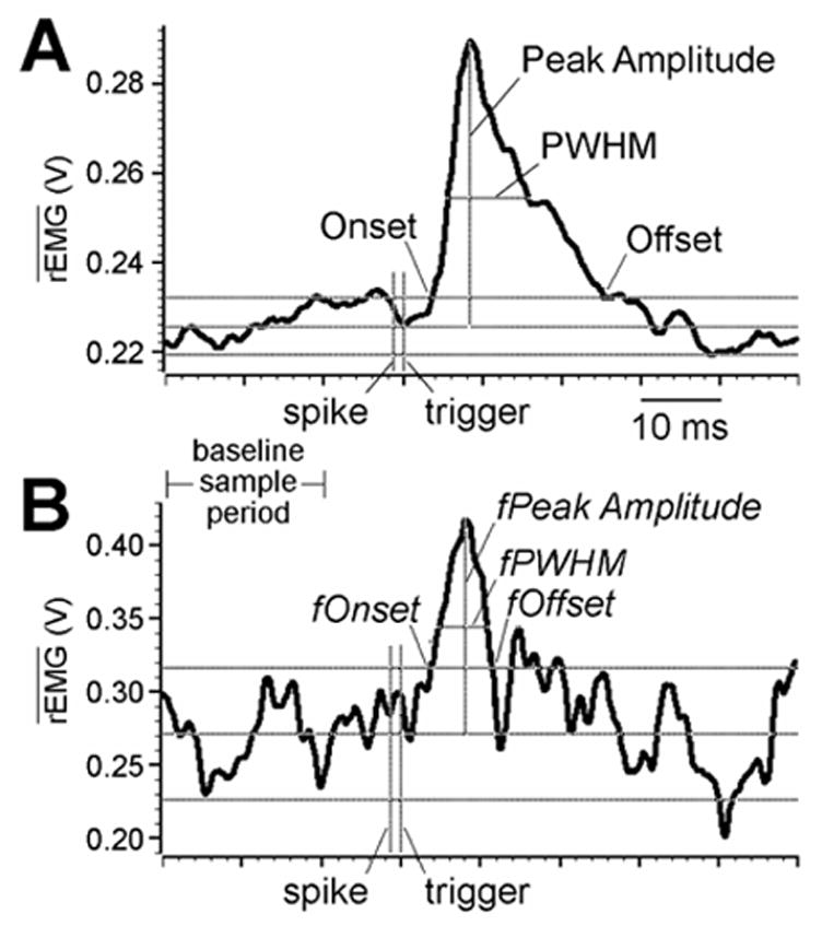
Measurements made on SpikeTAs. A shows an 80 ms SpikeTA of rectified EMG from FDPu compiled from 24,470 EMG-filtered spikes discharged by neuron e0030 during an RPD epoch. Three horizontal lines indicate the levels of the mean ± 2 standard deviations (SDs) of the SpikeTA during the baseline sample period. The points at which the SpikeTA crosses the ± 2 SDs line before and after the peak define the Onset and Offset, of the SpikeTA effect respectively. A separate horizontal line segment indicates the peak width at half maximum (PWHM) of the SpikeTA effect. Three vertical line segments indicate the time of the beginning of the spike (action potential), the time of the trigger pulses used to align data for averaging, and the Peak Amplitude above the baseline sample period mean. Algorithms for making these and other measurements are described in the Methods. B shows an 80 ms fragment SpikeTA compiled from only 100 of the spikes that contributed to the overall SpikeTA in A. As described in the Results, the same algorithms used to measure features of the overall SpikeTA were used to measure features of the fragment SpikeTA. The ordinates in A and B have been scaled to fill the same vertical height from minimum to maximum of the SpikeTA waveforms. For both A and B, units of average rectified EMG ( $\overline{\text{rEMG}}$) are in Volts after amplification 10,000x.

Results

Removing baseline trends with Increment-Shifted Averages

Figure 2 shows initial SpikeTAs of 6 neuron-muscle pairs selected to illustrate a variety of baseline trends. For each neuron-muscle pair, the left column shows the initial SpikeTA with the vertical scale adjusted to show the entire trace relative to zero average rectified EMG activity ( $\overline{\text{rEMG}}$). The brief peak or trough following the trigger time (vertical line) in these examples represents the increase or decrease in $\overline{\text{rEMG}}$ that results from short-latency synaptic input to the motoneuron pool time-locked to the spikes discharged by the trigger neuron. We refer to these peaks and troughs as SpikeTA effects. Each SpikeTA effect can be seen to ride on a baseline of $\overline{\text{rEMG}}$, which represents the average ongoing EMG activity around the time the trigger neuron discharged spikes. Although SpikeTAs used for standard analyses typically are 80 ms long, here the initial SpikeTAs are shown for 160 ms to emphasize the underlying baseline trends. Whereas in the uppermost SpikeTA this baseline is reasonably flat (A), the $\overline{\text{rEMG}}$ baseline may show an approximately linear trend (ramp) that either rises (B) or falls (C), or may be overtly curvilinear with convexity either up (D) or down (E). In some cases, the baseline undergoes a sudden inflection at the time a SpikeTA effect might occur (F).

Figure 2.

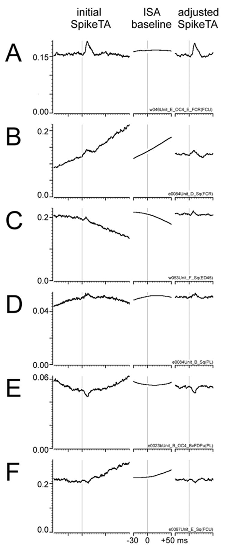
Adjustment of baseline trends with Increment Shifted Averages. A-F show SpikeTAs from 6 different neuron-muscle pairs with various baseline trends: A – flat; B – rising ramp; C – falling ramp; D – convex up; E – convex down; F – inflection. The left column shows the initial SpikeTA for each neuron-muscle pair. To reveal the baseline trends more clearly, in this column 160 ms are shown, although analyses typically are performed on SpikeTAs 80 ms in duration. The middle column shows the increment shifted average (ISA) estimate of the baseline trend during the 80 ms period used for analysis. The right column shows the 80 ms ISA-adjusted SpikeTA. Note that in these adjusted SpikeTAs the baseline trend has been effectively flattened, without reducing the stochastic noise of the SpikeTA or altering the height of the SpikeTA above 0. For each neuron-muscle pair A – F, the same ordinate scale at left ( $\overline{\text{rEMG}}$ in Volts after amplification) applies to all three averages in the row: initial SpikeTA, ISA baseline, and adjusted SpikeTA. A vertical hairline has been drawn at the trigger time for each average. Time scales beneath each average show major tick marks at the trigger time (0 ms), and at −30 ms and +50 ms (the 80 ms analysis window), with minor tick marks every 5 ms.

These baseline trends represent the average pattern of co-modulation of neuron firing rate and EMG activity. A rising baseline trend (B), for example, indicates that the neuron tended to discharge spikes at times of increasing EMG, such that on average more EMG activity occurred after a spike than before. Conversely, a falling baseline (C) indicates that the neuron tended to discharge spikes at times of decreasing EMG, such that on average more EMG activity occurred before a spike than after. Convex up curvilinear baseline trends (D) indicate that the neuron tended to discharge spikes during phasic bursts of EMG; whereas convex down trends (E) indicate that the neuron tended to discharge spikes between EMG bursts. Inflections in the baseline (F) indicate that the neuron tended to fire spikes when a steady level of EMG activity changed abruptly. The patterns of neuron-EMG co-modulation reflected by these baseline trends occur on a time scale an order of magnitude longer than the spike-locked synaptic inputs responsible for the ~10 – 20 ms peaks and troughs that follow the trigger time, i.e. the SpikeTA effects.

In order to quantify the features of a SpikeTA effect accurately, any baseline trend in the $\overline{\text{rEMG}}$ reflecting long-term neuron-EMG co-modulation should be removed, for two reasons. First, in computing the peak percent increase (PPI) and mean percent increase (MPI), the baseline level of $\overline{\text{rEMG}}$ is used to normalize the amplitude of the peak or trough. A rising or falling trend in the period used to estimate the baseline level of $\overline{\text{rEMG}}$ would alter the values computed for PPI and MPI. For example, a rising trend preceding a SpikeTA effect would result in a lower estimate of the baseline level than a falling trend preceding the same SpikeTA effect. Second, the onset and offset times of the SpikeTA effect are identified when the peak or trough crosses some pre-defined level, typically set at ± 2 standard deviations from the baseline period mean. A rising or falling trend during the baseline sample period would increase the standard deviation of the baseline during that period. The larger standard deviation would result in onset and offset times closer to the maximum or minimum of the peak or trough, respectively, than for the same SpikeTA effect riding on a flat baseline.

Linear rising and falling trends customarily have been removed by calculating a best-fit line through a period of the SpikeTA that samples the baseline trend but not the SpikeTA effect per se (Lemon, Mantel et al., 1986; McKiernan, Marcario et al., 2000). This line then is subtracted from the initial SpikeTA, which flattens the baseline but also brings the average value down to zero. A constant (e.g. the original value of the SpikeTA at the trigger time) therefore is added back to the SpikeTA to restore the height of the baseline $\overline{\text{rEMG}}$ above zero. This procedure removes a linear baseline trend while preserving the stochastic noise level of the SpikeTA waveform.

The ramp subtraction approach fails to remove curved baseline trends, however. We therefore developed a method of removing an arbitrary curvilinear baseline trend, while making no assumptions about the shape of that trend or the characteristics of any spike-locked effects. Figure 3A shows simultaneously recorded neural activity from a microelectrode in M1 and EMG activity from EDC. During this period the largest spike in the M1 recording discharged three times, generating three triggers that were used in forming a SpikeTA. These three triggers discriminated from the spike are shown in Figure 3B, along with the three corresponding segments of full-wave rectified EMG. These three segments of rectified EMG were aligned along with 6,011 additional segments around other spike triggers from the same neuron, and averaged to form the initial SpikeTA shown on the left in Figure 3D below.

Figure 3.

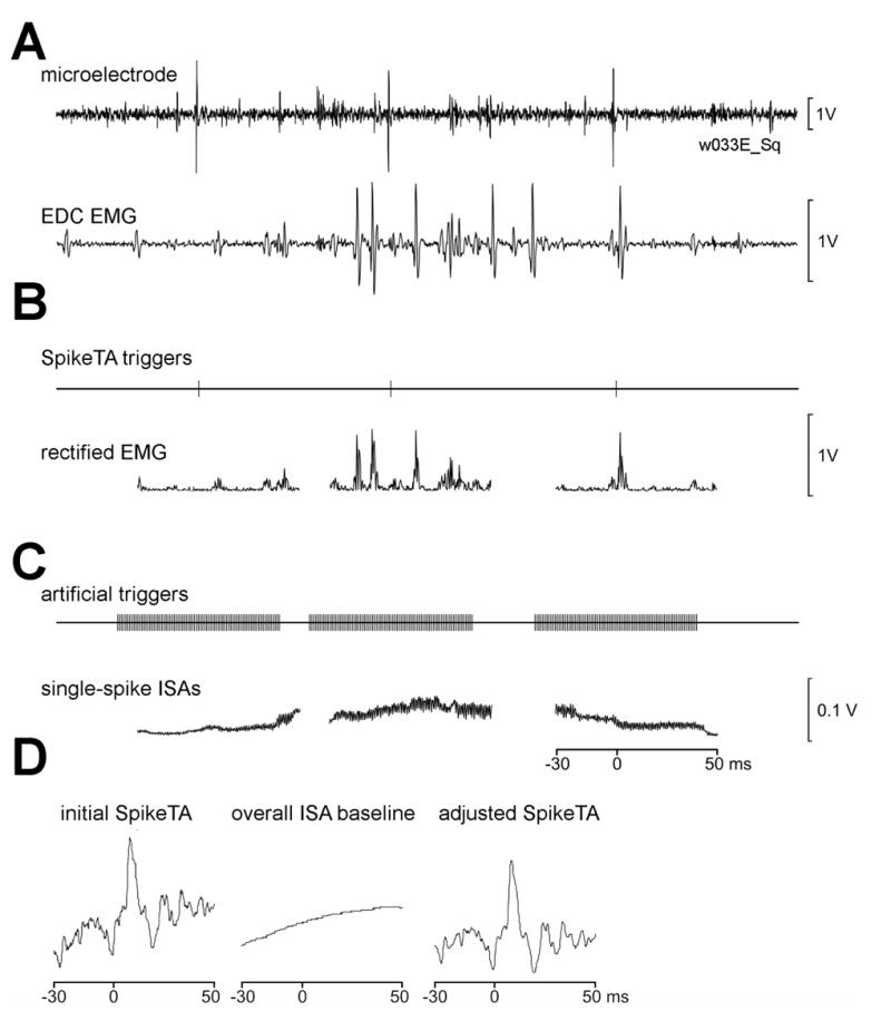
Increment shifted averaging to estimate the baseline trend. A. A short segment of a microelectrode recording shows three large spikes discharged by a neuron. EMG recorded simultaneously from EDC is shown below. B. Triggers from each of the three neuron spikes in A are are shown above, and corresponding segments of full-wave rectified EMG are shown below. C. For each of the three SpikeTA triggers in B, 81 artificial triggers were generated at increments of 1 ms, from 40 ms before to 40 ms after the SpikeTA trigger. These 81 artificial triggers were used to define corresponding segments of rectified EMG which then were aligned and averaged to compile the single-spike increment shifted averages (ISAs) shown below. The 1kHz periodicity of the single-spike ISAs reflects the 1 ms interval between artificial triggers. Nevertheless, the noise level of the single-spike ISAs shown in C is substantially lower than the variability of the full-wave rectified EMG shown in B (note vertical scales at right). All data in A, B and C are aligned in time (scale in C). D. The initial SpikeTA for this neuron-muscle pair compiled from 6,014 segments of rectified EMG like the three illustrated in B showed a rising curvilinear baseline (left). This baseline was captured by the overall ISA (center), compiled from 6,014 corresponding single-spike ISAs, like the three shown in C. Subtraction of the overall ISA from the initial SpikeTA produced the adjusted SpikeTA (right) with a relatively flattened baseline but preserved stochastic noise level.

Our method of removing an arbitrary curvilinear baseline trend is illustrated in Figure 3C. Eighty-one artificial triggers were created at 1 ms intervals starting 40 ms before and ending 40 ms after each spike of the trigger neuron used to form the initial SpikeTA. The artificial triggers created around each of the three triggers shown in Figure 3B are illustrated in Figure 3C. Segments of rectified EMG beginning 30 ms before and ending 50 ms after each of these 81 artificial triggers then were aligned and averaged to create a single-spike increment shifted average (ISA), as illustrated in Figure 3C. The time sampled by a single-spike ISA thus extended from 30 ms before the first of the 81 artificial triggers to 50 ms after the last. The 1 kHz periodicity in the single-spike ISAs reflects the 1 ms increment used to generate these moving averages.

This approach distributes any spike-locked change in EMG evenly over the single-spike ISA, while capturing any baseline trend on the scale of 80 ms or more. The three single-spike ISAs shown in Figure 3C each capture the general trend in EDC EMG activity at the time each of the three spikes was discharged by the M1 trigger neuron. The first of these three spikes was discharged when EMG was relatively low but increasing; the second when EMG was higher and peaking, and the third when EMG was decreasing.

All 6,014 single-spike ISAs associated with the 6,014 spikes from the trigger neuron then were averaged together, resulting in an overall ISA estimate of the baseline trend, shown as the center trace in Figure 3D. This overall ISA was subtracted from the initial SpikeTA (Figure 3D left), and the value of the initial SpikeTA at the trigger time was added back to restore the baseline level above zero (not shown here), resulting in the ISA adjusted SpikeTA shown on the right of Figure 3D. This procedure eliminated the curvilinear rising baseline trend from the adjusted SpikeTA.

Additional examples of overall ISA baseline estimates and adjusted SpikeTAs are shown in the middle and right columns, respectively, of Figure 2. Note that whereas the initial SpikeTAs in Figure 2 (left) are shown for 160 ms to emphasize the baseline trends, the ISA baselines (center) and adjusted SpikeTAs (right) are 80 ms in duration, the duration of the SpikeTAs used for measurement of SpikeTA effects. Each ISA captures the baseline trend of each initial SpikeTA, while eliminating the brief peak or trough of the SpikeTA effect per se. In addition, because the ISA averages 81 EMG samples for each EMG sample used in the initial SpikeTA, the noise level of the ISA is markedly lower, and therefore the ISA-adjusted SpikeTA preserves the noise features of the initial SpikeTA.

For SpikeTAs in which the baseline trend is highly linear (e.g. Figure 1 A, B and C) the present ISA method has no advantage over linear ramp subtraction. As the baseline trend comes to include more curvature (e.g. Figure D, E and F), however, subtraction of a linear ramp fails to remove curvature from the baseline trend preceding the SpikeTA effect, as well as from the baseline trend underlying the SpikeTA effect (peak or trough) itself. Such curvature contributes extra variation to the baseline preceding the trigger time, producing inaccurate measurements of onset and offset of the SpikeTA effect. Furthermore, baseline trend curvature at the time of the SpikeTA effect itself results in over- or under-estimation of the amplitude of the SpikeTA effect. Using the ISA to adjust the baseline of the SpikeTA results in more accurate measurement of both the amplitude and temporal characteristics of the SpikeTA effect. ISA adjustment therefore has been applied to all SpikeTAs described below.

Identifying changes in SpikeTA effects with a Multi-Fragment Approach

Figure 4A shows two ISA-adjusted SpikeTAs compiled for the same neuron-muscle pair (e0030-FDPu) during the squeeze task (left) and during RPD of the neuron versus the muscle (right), both displayed on the same vertical scale. Both SpikeTAs show a clear post-spike facilitation (PSpF). Whereas the baseline levels of average EMG are similar, the PSpF on the right appears to be larger than that on the left, and appears longer in duration as well. Indeed, during the squeeze task, the PSpF had a measured PPI of 12.7% and a PWHM of 6.1 ms, whereas during RPD the PSpF had a PPI of 28.5% and a PWHM of 9.5 ms. Given that the squeeze SpikeTA was compiled from 16,109 EMG-filtered triggers, and the RPD SpikeTA from 24,470, one would expect these differences in PPI and PWHM to be genuine. But are these differences significant, or might they have arisen by chance alone?

Figure 4.

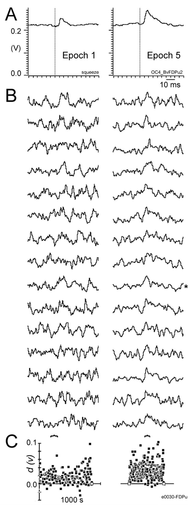
A. SpikeTAs compiled for the same neuron-muscle pair during two different behavioral epochs are shown on the same vertical scale (Volts after amplification 10,000x). Left, Epoch 1 – squeeze task; Right, Epoch 5 – RPD of neuron e0030 versus FDPu. Both SpikeTAs are 80 ms in duration. B. Fifteen sequential fragment spike-triggered averages (fSpikeTAs), each compiled from 100 sequential spikes, are shown from Epoch 1 (left) and from Epoch 5 (right). Each fSpikeTA is scaled to fill the same vertical height from minimum to maximum, and is 80 ms in duration. C. The test statistic, d, is plotted as a function of time for each of the fragments from Epoch 1 (left) and Epoch 5 (right). The time at which each d value is plotted is the time at which that fragment ended. The time scale of 1000 s (left) applies to both epochs. Values of d for the 15 fSpikeTAs shown in B are indicated with horizontal curly brackets.

We previously have used a multi-fragment approach to identify significant peaks or troughs in SpikeTAs (Poliakov and Schieber, 1998). The spike train used to compile the SpikeTA is divided into multiple non-overlapping fragments, each including the same number of spikes, and a separate SpikeTA is compiled using the spikes in each fragment, resulting in multiple fragment spike triggered averages (fSpikeTAs). From each fSpikeTA, a test statistic, d, is calculated as the mean value in a temporally fixed test window (chosen to encompass the typical peak or trough times of SpikeTA effects), minus the mean in two control windows that immediately precede and follow the test window. The test statistic, d, thus assays whether the $\overline{\text{rEMG}}$ in the test window is systematically different from that in the flanking control windows. If d is statistically different from 0 across all the fragments, then we reject the null hypothesis that no peak or trough exists in the test window, and accept the peak or trough in the overall SpikeTA as significant.

Figure 4B shows 15 sequential ISA-adjusted fSpikeTAs, each compiled with 100 sequential EMG-filtered spikes during the squeeze task (left) and RPD (right). Each fSpikeTA is scaled to fill the same vertical height. Peaks in the fSpikeTAs corresponding in time to the peak in the overall SpikeTAs shown above in A are more evident in the RPD fSpikeTAs (right). Even though peaks are not obvious in the squeeze task fSpikeTAs (left), the same phenomena underlying the obvious peak in the overall SpikeTA can be assumed to be present, on average, in these fSpikeTAs.

Figure 4C (left) shows values of d (test window 6 to 16 ms after the trigger) for all 161 fSpikeTAs from the squeeze task (left). While not apparent upon visual inspection of the 15 fSpikeTAs shown above in Figure 4B, Figure 4C shows that on average d was greater than 0. Furthermore, although the values of d from successive fSpikeTAs might be considered a time series, and therefore not independent of one another, Figure 4C shows that the variability of d was greater than any temporal trend. Indeed, the correlation between each value of d and its predecessor gave a correlation coefficient of r = 0.11 for the squeeze task and r = 0.12 for the RPD task, providing little suggestion that the successive d values depend on one another within either epoch.

Because the distribution of d often was significantly different from normal (Lilliefors test, P < 0.05), we used the Wilcoxon signed rank test to determine whether the median value of d was significantly different from 0. Applying this test to the 161 d values from squeeze task fSpikeTAs (Figure 4C, left), and to the 244 d values from the RPD task (Figure 4C, right) confirmed that the PSpF peaks in both overall SpikeTAs (Figure 4A) were significant (squeeze task P = 2.3x10⁻²³, RPD task P = 1.2x10⁻⁴¹).

We now extend this approach to compare measured amplitude and temporal features of SpikeTA effects obtained during different behaviors. The peak percent increase (PPI) of a SpikeTA effect is a standard measure of the amplitude of the peak (or trough) normalized as a percentage of the baseline EMG preceding the trigger time in the SpikeTA. As for d, even when no peak or trough is evident above the noise in a given fSpikeTA, we can measure a peak percent increase for the fragment. First, the mean value of the fSpikeTA in the baseline sample period (from 30 to 10 ms before the trigger time, see Figure 1B) is subtracted from the mean value in the test window 6 to 16 ms after the trigger. If the result is positive (negative), a peak (trough) is assumed to be present. The fSpikeTA baseline mean is subtracted from the maximum (minimum) in the test window, providing a measure of the peak amplitude for the fragment. This fragment peak amplitude then is divided by the baseline mean and multiplied by 100, normalizing the peak amplitude as a percentage of the baseline mean, the fragment PPI, fPPI. This fPPI then can be used as a test statistic to compare PPIs of overall SpikeTAs compiled during different behavioral epochs.

The fPPIs of all fragment SpikeTAs from neuron-muscle pair e0030-FDPu are shown in Figure 5B as a function of time. Neuron-muscle pair e0030-FDPu was recorded during nine behavioral epochs. (Data from epochs 1 and 5 were shown in Figure 4.) The overall ISA-adjusted SpikeTA compiled for each epoch is shown above in Figure 5A. To facilitate comparison of PPI in the nine epochs, here the vertical scale of each of the nine SpikeTAs has been adjusted separately to match the heights of the baselines above zero. Note that the SpikeTA effect of this neuron-muscle pair was particularly strong during epochs 3 and 5, PPIs for these two overall SpikeTAs being 30.0% and 28.5%, respectively.

Figure 5.

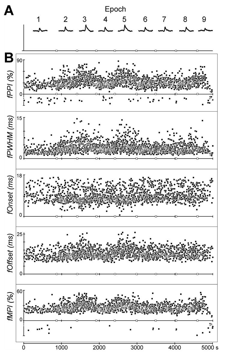
A shows SpikeTAs for neuron-muscle pair e0030-FDPu compiled for each of nine successive behavioral epochs: 1) Squeeze task; 2) RPD of neuron e0030 versus FCR; 3) e0030 v FDPu; 4) e0030 v FCR; 5) e0030 v FDPu; 6) e0030 v APL; 7) e0030 v ECRB; 8) e0030 v FCU; 9) e0030 v FDPu. To facilitate visual comparison of the peaks, here these nine SpikeTAs have been scaled individually to match the baseline level of EMG relative to zero. The abscissa time scale is 5000 s overall (scale at bottom of Figure), with the points at which behavioral epochs changed indicated with open squares. B shows test statistics fPPI, fPWHM, fOnset, fOffset, and fMPI for each fSpikeTA plotted as a function of time. Each value is plotted at the time at which the last spike of that fragment occurred. Abcissas again are 5000 s long, with tics every 1000 s, and open squares at the borders between behavioral epochs.

As for d, the variability of fPPI within a given epoch was substantially greater than any temporal trend within that epoch. This fragment-to-fragment variability primarily reflects variability in the behavior sampled during the relatively brief periods represented by individual fSpikeTAs, in the present example averaging 2.8 sec (range 1.5 to 33.4 sec). In spite of this variability, differences between certain epochs were evident. For example, fPPI values were systematically greater in epochs 3 and 5 than in epoch 1.

Because fPPIs in individual epochs were not normally distributed, we used the Kruskal-Wallis test of the null hypothesis that PPI did not vary among epochs. This hypothesis was rejected (P = 0). Post-hoc pairwise comparisons also confirmed that PPI in epoch 1 differed from that in epochs 3 and 5 (Wilcoxon rank sum tests, P = 1.4x10⁻³⁰ and P = 1.1x10⁻³¹). We therefore can conclude that the values of PPI measured in the overall SpikeTAs of epoch 1 (PPI = 12.7%) indeed was significantly different from that measured in epoch 3 or 5 (PPI = 30.0% and 28.5%, respectively). In contrast, post-hoc testing showed no significant differences between the PPIs of epochs 3 and 5, or among PPIs of epochs 2, 4, 6, 7, 8 and 9 (P > 0.0015, i.e. P > 0.05 after Bonferroni correction for 36 pairwise comparisons).

A similar multi-fragment approach can be used to evaluate changes in a measure of the temporal width of the SpikeTA effect, the peak width at half maximum (PWHM). PWHM is a useful measure of width because its measurement is affected less by the residual noise level of the SpikeTA than is the total duration of the peak or trough from onset to offset. Again, although a peak or trough may not be evident in each fragment SpikeTA, the same algorithm used to measure the PWHM of an overall SpikeTA can be applied to each fSpikeTA (see Figure 1B) The level halfway from the baseline period mean to the maximum (minimum) in the test window is determined (half the peak amplitude). The fSpikeTA then is followed both backward and forward from the maximum (minimum) to find the times at which the fSpikeTA crosses the half-maximum level before and after the maximum (minimum), and the difference between these two times provides a measure of the PWHM for the fragment, fPWHM, which can be used as a test statistic for comparing PWHMs. Figure 5B shows the fPWHMs for e0030-FDPu as a function of time. As for fPPI, categorizing these data according to the nine behavioral epochs and applying a Kruskal-Wallis test confirmed that PWHM varied across epochs (P = 0). Post-hoc testing confirmed that the PWHMs of 9.0 ms in epoch 3 and 9.5 ms in epoch 5 differed significantly from the PPI of 6.1 ms in epoch 1 (Wilcoxon rank sum tests, P = 3.2x10⁻²⁶ and 6.9x10⁻²⁵).

Additional SpikeTA effect measures—mean percent increase (MPI), onset time and offset time—also can be compared using the multi-fragment approach, subject to one caveat. Our algorithm for assessing these features requires that a fSpikeTA exceed 2 standard deviations (SDs) from its baseline mean during the test window. Then the fSpikeTA can be traced both backward and forward to its 2 SDs level to find the onset and offset times (fOnset and fOffset)of the fSpikeTA, respectively (see Figure 1B). An MPI for the fragment (fMPI) then is computed between the fOnset and fOffset. In some fragments the fSpikeTA may not exceed 2 SDs during the test window. For such fragments, fOnset and fOffset, and consequently fMPI, cannot be determined. Nevertheless, the fragments in which the SpikeTA does exceed 2 SDs from the baseline mean still can be used to measure fOnset, fOffset, and fMPI. Figure 5 shows fOnset, fOffset, and fMPI for all measurable fragments from e0030-FDPu as functions of time. Each of these test statistics varied significantly across the nine behavioral epochs, permitting us to reject the null hypotheses that the Onset, Offset and MPI of the overall SpikeTA effects shown above in Figure 5A did not vary among epochs (Kruskal-Wallis tests: Onset P = 6.0x10⁻¹⁵; Offset P = 0; MPI, P = 0). Comparing epoch 1 with epoch 5 specifically, post-hoc testing confirmed significant differences in MPI (7.1% vs 12.7%, P = 2.8x10⁻²¹) and Offset time (17.4 ms vs 29.4 ms, P = 1.4x10⁻¹³), but not in Onset time (5.4 ms vs 4.6 ms, P > 0.0015)(Wilcoxon rank sum tests).

Values of fragment test statistics correlate with values measured in overall SpikeTAs

While fPPI, fPWHM, fMPI, fOnset, and fOffset are used as test statistics, the average values of these test statistics do not equal the values of PPI, PWHM, MPI, Onset and Offset, respectively, measured from the overall SpikeTAs. Differences result from the fact that the residual noise level of each fSpikeTA will be greater than that of the overall SpikeTA. As illustrated in Figure 1B, the higher noise level will result in a higher peak (lower trough) value of the fSpikeTA maximum (minimum), resulting in a tendency for fPPIs to be systematically greater than the corresponding PPI measured for the single overall SpikeTA. Furthermore, because the higher noise level of the fSpikeTAs moves the ± 2 standard deviation levels further from the baseline period mean, fOnsets will be found systematically later, and fOffsets systematically earlier, (both closer to the time of the maximum (minimum)) than the Onset and Offset times for the overall SpikeTA. And because the fOnsets and fOffsets will be closer to the time of the maximum (minimum), fMPIs will tend to be larger than the MPI measured in the overall SpikeTA. Similarly, the times at which the SpikeTA crosses the half maximum level before and after the maximum (minimum) both will be closer to the maximum (minimum), and consequently fPWHMs will tend to be shorter than PWHM measured in the overall SpikeTA.

Nevertheless, if the fragment test statistics reflect the same underlying process revealed in the overall SpikeTA, the test statistic values averaged across all the fragments of a given epoch should be correlated with the value measured from the overall SpikeTA. Figure 6A shows scatter plots of average fPPI plotted against the PPI of the overall SpikeTA effect, and of average fMPI plotted against the overall MPI, for neuron-muscle pair e0030-FDPu in the 9 epochs illustrated in Figure 5. Figure 6B shows similar plots for PWHM, Onset and Offset. For all five of these parameters, the average of values measured from fSpikeTAs was correlated with the value measured from the overall SpikeTA (correlation coefficients: PPI, 0.97; MPI, 0.91; PWHM, 0.86; Onset, 0.80; Offset, 0.86), and linear regression showed a slope significantly different from 0 (P < 0.01, or P < 0.05 after Bonferonni correction for 5 tests). These observations support use of the fragment test statistics for comparison of measurements made on the overall SpikeTA effects.

Figure 6.

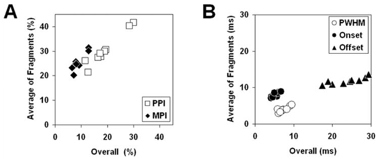
Correlations between test statistics and measures of overall SpikeTA effects. Scatterplots illustrate the correlations between the average of fragment test statistics (ordinate: fPPI, fMPI, fPWHM, fOnset and fOffset) and measurements of amplitude (A) and temporal (B) features of SpikeTA effects (abscissa: PPI, MPI, PWHM, Offset and Onset, respectively) made from the overall SpikeTAs during nine different behavioral epochs for neuron-muscle pair e0030-FDPu.

Selecting the number of spikes per fragment

The multi-fragment approach entails a trade-off between the number of spikes per fragment and the number of fragments. The more spikes allotted to each fragment, the better the peak-to-noise ratio of each fSpikeTA, but the fewer the number of fragments. In the limit of having too few fragments (samples), statistical testing may not show significance, even in the presence of clear SpikeTA effects. As a reasonable compromise between these two extremes, for a recording that included a total number, N, of EMG-sweep filtered spikes, we previously chose to use $\sqrt{N}$ fragments, each with $\sqrt{N}$ spikes to test an individual SpikeTA for the presence of a SpikeTA effect (Poliakov and Schieber, 1998).

In the present study, however, we endeavor to compare SpikeTAs compiled for the same neuron-muscle pair during different epochs, a condition under which the number of EMG-filtered triggers available typically differs among epochs. Using $\sqrt{N}$ then would result in different numbers of spikes per fragment in different epochs. The peak-to-noise ratio of the fSpikeTAs would vary among epochs simply because different numbers of spikes per fragment would be used in analyzing different epochs. We therefore chose here to use a fixed number of spikes per fragment. Because our epochs typically contained ~10,000 spikes, we chose to fix the number of spikes per fragment at 100 (close to $\sqrt{N}$). In this way, although the number of fragments might vary among epochs, the peak-to-noise ratio of the fSpikeTAs remains unaffected by differences in the number of spikes in various epochs.

To examine the effect of the number of spikes per fragment (hereafter abbreviated as n) and of the number of fragments (ν = N/n) on the outcome of multi-fragment analysis, we repeated the analysis using different n. The results are illustrated in Figure 7 for a neuron-muscle pair (e0030-Thenar) which showed clear SpikeTA effects in some behavioral epochs, but no SpikeTA effect in others (Figure 7A). Figure 7B and 7C shows how the P-value obtained for the presence of a significant peak (test-statistic d, Wilcoxon signed rank test) varied when we used n = 25, 50, 100, 200, 400, 800, 1600, or 3200 spikes per fragment. As expected, P-values generally were closer to 1 for larger n (Figure 7B) and smaller ν (Figure 7C), and fell toward 0 as n was reduced increasing ν. Note, however, that for epochs 1 and 7 the SpikeTAs of which have no substantial peak, the P-value never fell below 0.1. Neither of these epochs would have been considered to have a significant SpikeTA effect using any value of n, even using a small n to produce a large ν. Epoch 9 provides an instructive borderline example. Visual inspection of the epoch 9 SpikeTA shown in Figure 7A suggested a questionable peak at the time a SpikeTA effect would be expected (*), but this peak was not substantially larger than features at other times in the same SpikeTA (^). As n was Page 27 reduced from 3200 to 25, increasing ν from 2 to 281, the P-value for epoch 9 fell from levels that could not be considered significant, through levels typically used as criteria for significance. With a criterion set at P < 0.005 (0.05 after Bonferonni correction for the 9 tests on 9 epochs), the SpikeTA of epoch 9 would not have been considered significant using n >100, but would have been considered significant using n≤ 100 (ν≥ 89). Using the same criterion (P < 0.005), the SpikeTA effects of the remaining epochs (2, 3, 4, 5, 6, 8) all would be considered significant using n ≤ 400 (ν≥ 41). Had these epochs with more obvious SpikeTA effects not been available, one would doubt the presence of an effect in epoch 9, but in view of the evident effect for this neuron-muscle pair in several epochs, the effect in epoch 9 might be considered marginally genuine.

Figure 7.

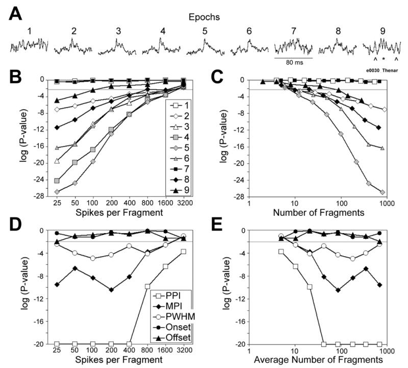
Effect of the number of spikes per fragment and of the number of fragments on P-values. A. SpikeTAs from nine behavioral epochs are shown for a neuron-muscle pair selected for the presence of a clear SpikeTA effect in several epochs (2, 3, 4, 5, 6, and 8), no effect in other epochs (1 and 7), and a borderline effect in one epoch (9). For the SpikeTA in epoch 9, a questionable peak might be present (*), but features of similar size are present at other times (^). All nine SpikeTAs are scaled to fill the same vertical height from minimum to maximum, and are 80 ms in duration. The P-value obtained testing the null hypothesis that no SpikeTA effect (peak) is present is shown as a function of the number of spikes per fragment in B, and as a function of the number of fragments in C, for each of the nine epochs (test-statistic d, Wilcoxon signed rank test). A horizontal line has been drawn in B and C at P = 0.005 (0.05 after Bonferonni correction for the 9 tests on 9 epochs), and the legend in B applies to C as well. The P-value obtained testing the null hypotheses that measured parameters of the SpikeTA effects (PPI, MPI, PWHM, Onset and Offset) did not change across behavioral epochs is shown for each parameter (test statistics fPPI, fMPI, fPWHM, fOnset and fOffset, respectively; Kruskal-Wallis tests) as a function of the number of spikes per fragment in D and as a function of the average number of fragments across the nine epochs in E. A horizontal line has been drawn in D and E at P = 0.01 (0.05 after Bonferonni correction for 5 tests). A floor of log(P) = −20 was used to permit better visualization of these results for parameters other than PPI. The legend in D applies to E as well Note that in B, C, D and E both abscissa and ordinate are logarithmic scales.

Figure 7D and 7E shows how the P-value obtained for variation among the nine epochs in measured parameters PPI, MPI, PWHM, Onset and Offset (test statistics fPPI, fMPI, PWHM, fOnset and fOffset; Kruskal-Wallis tests) changed when we used different n, and consequently different ν, respectively. With a criterion of P < 0.01 (P < 0.05 after Bonferonni correction for 5 tests), neither Onset nor Offset would have been considered to vary significantly among epochs using any n. With the same criterion, PWHM, MPI and PPI all would have been considered to vary significantly using any n < 3200 (average ν > 10).

Using a small n and a large ν thus will result in more SpikeTA effects, and more changes among epochs, being accepted as significant for any fixed criterion P-value. Using a large n and a small ν may result in some genuine SpikeTA effects and some real variation among epochs being rejected. For our present data, n = 100 appeared to be a reasonable compromise between these two extremes.

Discussion

We have introduced two approaches to improve comparison of effects in spike-triggered averages (SpikeTAs) of rectified EMG across different behaviors. First, we have used an increment shifted average (ISA) to remove arbitrary curvilinear trends in the baseline of the SpikeTA. Second, we have extended the multiple fragment statistical approach to compare features of SpikeTA effects. These two approaches permit more accurate comparison of SpikeTA effects produced at different times by the same neuron-muscle pair

Correcting for baseline trends

A SpikeTA effect represents spike-locked changes in motor unit discharge probability that occur over several milliseconds after synaptic input to the motoneuron pool. In contrast, the baseline trend of the SpikeTA represents co-modulation of the neuron spike train with the envelope of EMG activity occurring over hundreds of milliseconds. When baseline trends are approximately linear, a best-fit line can be used to remove the trend. But in a certain number of cases, the SpikeTA baseline trend shows overt curvature. Curvilinear baseline trends pose a number of problems. If the baseline trend peaks or inflects in the time window when a SpikeTA effect could occur, the spike-locked effect may be discarded as being part of the baseline trend. Alternatively, a broad curvature or inflection in the baseline trend may be mistaken for a spike-locked effect. Moreover, if the baseline curvature is not removed, values measured for PPI, MPI, PWHM, Onset and Offset of the SpikeTA effect will be inaccurate, and difficult to compare among behavioral epochs. Use of the ISA to correct for the baseline trend ameliorates these problems without requiring a priori selection of a linear or polynomial model of the baseline trend.

We also considered two other possible algorithms for estimating the underlying baseline trend in SpikeTAs. We considered forming an average by assigning artificial triggers at times randomly selected within some window around each trigger used for the SpikeTA. Although this approach jitters the spike-locked EMG randomly, unless very large numbers of randomly chosen trigger times are used, the spike-locked EMG may not be evenly distributed in such a jittered average. Because using substantially more than 80 artificial triggers for each actual SpikeTA trigger dramatically increased the computational time required, we prefer the ISA, which provides a similar result faster.

The ISA is a form of moving average filter that has the effect of removing high frequency components from the SpikeTA to reveal the baseline trend. We therefore considered the alternative possibility of high-pass filtering the SpikeTA to reject the lower frequency baseline trend while preserving higher frequency components that include both the SpikeTA effect and the residual noise. This approach produces results similar to the ISA for many SpikeTA effects. Some SpikeTAs show atypical spike-locked effects, however, such as very broad synchrony effects or slow oscillations. The fundamental frequencies of such atypical effects lie between those of typical SpikeTA effects and curvilinear baseline trends. Hence such spike-locked effects are difficult to separate reliably from the baseline trend by filtering in the frequency domain. We therefore prefer the ISA, which accounts consistently for any spike-locked features in the SpikeTA.

Comparing SpikeTA effects

We also extended the multiple fragment approach to compare measured parameters of SpikeTA effects—PPI, MPI, PWHM, Onset and Offset—in SpikeTAs compiled from data collected during two or more behavioral epochs. Test statistics for each parameter—fPPI, fMPI, fPWHM, fOnset and fOffset—were measured from multiple fragment SpikeTAs (fSpikeTAs). As these test statistics often were not distributed normally, rank order tests were used to compare values from different behavioral epochs. Because the fSpikeTAs inherently have a lower peak-to-noise ratio than the overall SpikeTA, the test statistics show considerable variation. Also due to the low peak-to-noise ratio, the average value of any given test statistic is not equal to the value measured from the overall SpikeTA. Nevertheless, the average of each test statistic correlates with the overall value.

The multiple fragment approach entails a tradeoff between the number of fragments, ν, and the number of spikes per fragment, n. To test the significance of a peak or trough in a single SpikeTA compiled from N spikes, we previously have parsed the available spikes into $\sqrt{N}$ fragments each compiled with $\sqrt{N}$ spikes. SpikeTAs compiled from data collected during two or more behavioral epochs typically will have different N, however, and using $\sqrt{N}$ spikes per fragment will cause the peak-to-noise ratio to differ among epochs based on this factor alone. We therefore chose here to fix the number of spikes per fragment, n, and examined the results obtained using different values of n. As n becomes large, approaching N, the number of fragments (ν = N/n) becomes small. With an excessively small number of fragments (samples), statistical tests become unable to reject the null hypothesis that no SpikeTA effect exists, or that no difference in SpikeTA effects exists. Conversely, as n becomes small, the number of fragments becomes large. With a large number of fragments (samples), statistical tests more readily reject the null hypothesis.

As illustrated in Figure 7, the multi-fragment approach can be very sensitive, both in detecting SpikeTA effects and in detecting changes in SpikeTA effects across different behavioral epochs. Because the P-values generated will depend in part on the number of spikes per fragment, this value should be chosen judiciously and applied consistently throughout an investigation. The criterion P-value chosen also should be recognized to be either relatively permissive or relatively restrictive. In addition, when investigating the SpikeTAs of large numbers of neuron-muscle pairs, and examining each for changes in multiple parameters, appropriate corrections for multiple tests (e.g. Bonferonni) should be applied.

By compiling SpikeTAs with spikes selected for different levels of background EMG activity, and correlating the amplitude of the resulting SpikeTA effects with the level of EMG activity, Bennett and Lemon (1994) demonstrated that the amplitude of the SpikeTA effect produced by some neuron-muscle pairs changed depending on the background level of EMG activity. This correlative approach provided a valuable test of the specific hypothesis that SpikeTA effect amplitude depended on background EMG level. But the correlative approach becomes less sensitive when only small numbers of SpikeTAs are available for comparison, and requires specific hypotheses about the factors producing variation in the SpikeTA effects.

In contrast, the multi-fragment approach can be used to compare as few as two SpikeTA effects, and permits statistical assessment of variation in SpikeTA effects among behavioral epochs without a priori assumptions about the factors contributing to the variation. Once significant variation is identified, further analysis is required to identify the contributing factors. Nevertheless, because variation in SpikeTA effects may reflect changes in the throughput from the spikes discharged by the trigger neuron to the EMG activity of its target muscles, the multi-fragment approach may provide a powerful tool for examining how pre-motoneuronal networks change to accomplish different behaviors.

References

- Baker SN, Lemon RN. Computer simulation of post-spike facilitation in spike-triggered averages of rectified EMG. J Neurophysiol. 1998;80:1391–406. doi: 10.1152/jn.1998.80.3.1391. [DOI] [PubMed] [Google Scholar]
- Bennett KM, Lemon RN. The influence of single monkey cortico-motoneuronal cells at different levels of activity in target muscles. J Physiol (Lond ) 1994;477:291–307. doi: 10.1113/jphysiol.1994.sp020191. [DOI] [PMC free article] [PubMed] [Google Scholar]
- Buys EJ, Lemon RN, Mantel GW, Muir RB. Selective facilitation of different hand muscles by single corticospinal neurones in the conscious monkey. J Physiol (Lond) 1986;381:529–49. doi: 10.1113/jphysiol.1986.sp016342. [DOI] [PMC free article] [PubMed] [Google Scholar]
- Cheney PD, Fetz EE. Comparable patterns of muscle facilitation evoked by individual corticomotoneuronal (CM) cells and by single intracortical microstimuli in primates: evidence for functional groups of CM cells. J Neurophysiol. 1985;53:786–804. doi: 10.1152/jn.1985.53.3.786. [DOI] [PubMed] [Google Scholar]
- Fetz EE. Operant conditioning of cortical unit activity. Science. 1969;163:955–8. doi: 10.1126/science.163.3870.955. [DOI] [PubMed] [Google Scholar]
- Fetz EE, Baker MA. Operantly conditioned patterns on precentral unit activity and correlated responses in adjacent cells and contralateral muscles. J Neurophysiol. 1973;36:179–204. doi: 10.1152/jn.1973.36.2.179. [DOI] [PubMed] [Google Scholar]
- Fetz EE, Cheney PD. Postspike facilitation of forelimb muscle activity by primate corticomotoneuronal cells. J Neurophysiol. 1980;44:751–72. doi: 10.1152/jn.1980.44.4.751. [DOI] [PubMed] [Google Scholar]
- Fetz EE, Finocchio DV. Operant conditioning of specific patterns of neural and muscular activity. Science. 1971;174:431–5. doi: 10.1126/science.174.4007.431. [DOI] [PubMed] [Google Scholar]
- Fetz EE, Finocchio DV. Operant conditioning of isolated activity in specific muscles and precentral cells. Brain Res. 1972;40:19–23. doi: 10.1016/0006-8993(72)90100-x. [DOI] [PubMed] [Google Scholar]
- Kasser RJ, Cheney PD. Characteristics of corticomotoneuronal postspike facilitation and reciprocal suppression of EMG activity in the monkey. J Neurophysiol. 1985;53:959–78. doi: 10.1152/jn.1985.53.4.959. [DOI] [PubMed] [Google Scholar]
- Lemon RN, Mantel GW, Muir RB. Corticospinal facilitation of hand muscles during voluntary movement in the conscious monkey. J Physiol (Lond) 1986;381:497–527. doi: 10.1113/jphysiol.1986.sp016341. [DOI] [PMC free article] [PubMed] [Google Scholar]
- McKiernan BJ, Marcario JK, Karrer JH, Cheney PD. Corticomotoneuronal postspike effects in shoulder, elbow, wrist, digit, and intrinsic hand muscles during a reach and prehension task. J Neurophysiol. 1998;80:1961–80. doi: 10.1152/jn.1998.80.4.1961. [DOI] [PubMed] [Google Scholar]
- McKiernan BJ, Marcario JK, Karrer JL, Cheney PD. Correlations between corticomotoneuronal (CM) cell postspike effects and cell-target muscle covariation. J Neurophysiol. 2000;83:99–115. doi: 10.1152/jn.2000.83.1.99. [DOI] [PubMed] [Google Scholar]
- Park MC, Belhaj-Saïf A, Cheney PD. Chronic recording of EMG activity from large numbers of forelimb muscles in awake macaque monkeys. J Neurosci Methods. 2000;96:153–60. doi: 10.1016/s0165-0270(00)00155-2. [DOI] [PubMed] [Google Scholar]
- Poliakov AV, Schieber MH. Multiple fragment statistical analysis of post-spike effects in spike-triggered averages of rectified EMG. J Neurosci Methods. 1998;79:143–50. doi: 10.1016/s0165-0270(97)00172-6. [DOI] [PubMed] [Google Scholar]
- Schieber MH. Training and synchrony in the motor system. J Neurosci. 2002;22:5277–81. doi: 10.1523/JNEUROSCI.22-13-05277.2002. [DOI] [PMC free article] [PubMed] [Google Scholar]
- Schieber MH, Rivlis G. A spectrum from pure post-spike effects to synchrony effects in spike-triggered averages of electromyographic activity during skilled finger movements. J Neurophysiol. 2005;94:3325–41. doi: 10.1152/jn.00007.2005. [DOI] [PubMed] [Google Scholar]