Molecular marker genotypes, heterozygosity and genetic interactions explain heterosis in Arabidopsis thaliana

Abstract

The underlying mechanisms for hybrid vigor or heterosis are elusive. Here we report a population of recombinant inbred lines (RILs), derived from the two ecotypes, Col and Ler, which can serve as a permanent resource for studying the molecular basis of hybrid vigor in Arabidopsis. Using a North Carolina mating design III (NCIII), we determined the additive and dominant nature of gene action in this population. We detected heterosis among crosses of RILs with one of the two parents (Col and Ler) and analyzed genotypes and heterozygosities for RILs and test cross families (RILs crossed to Col and Ler) using a total of 446 published molecular markers. The performance of RILs and additive and dominant components in the test cross families were used to analyze QTLs for 16 traits, using QTL cartographer and composite interval mapping with 1,000 permutations for each trait. Our data suggest that locus-specific and/or genome-wide differential heterozygosity, including epistasis, plays an important role in the generation of the observed heterosis. Furthermore, the hybrid vigor occurred between two closely related ecotypes, and provides a general mechanism for novel variation generated between genetically similar materials.

Introduction

Hybrid vigor or heterosis is one of the most fascinating phenomena in genetics, evolutionary biology and applied breeding. In general, hybrid vigor refers to the higher performance of an F₁ hybrid over the mean of the two parents. In agricultural sense, the F₁ should outperform the better parent to be useful. Heterosis has also been applied to adaptive traits like increased fecundity, viability and resistance to biotic and abiotic stress (Dobzhansky, 1950). In this report unless noted otherwise, we use heterosis in the agricultural sense for data analysis. Although breeders and farmers have long used hybrid varieties to produce high-yield and quality agricultural products, nonetheless the genetic basis for heterosis still remains unclear (Coors and Pandey, 1999). Therefore, understanding the underlying mechanisms is not only a great intellectual challenge but also has a promising applied side to it.

Two popular hypotheses, namely, dominance and overdominance, have stimulated interesting debates as to whether heterosis is caused by dominant complementation of slightly deleterious recessive alleles (Bruce, 1910; Jones, 1917; Xiao et al, 1995; Cockerham and Zeng, 1996) or by overdominant gene action in which genes have greater expression when they are heterozygous (Shull, 1908; East, 1936; Crow, 1948; Stuber et al, 1992; Mitchell-Olds, 1995). According to the former, highest performance should follow the maximum accumulation of dominant favorable genes from both parents in homozygous conditions. If the latter holds true, heterosis should reach its peak at the maximum levels of heterozygosity and dissipate when approaching homozygosity. In many cases, however, overdominance is accompanied by nonallelic interactions. Removing significant nonallelic interactions also results in reduction or disappearance of apparent overdominant effects (Jinks, 1955). The third model suggests that heterosis results from epistatic interactions among alleles at different loci. Indeed, epistasis is involved in most quantitative trait loci (QTLs) associated with inbreeding depression and heterosis in corn (Stuber et al, 1992) and rice (Li et al, 2001; Luo et al, 2001).

The relationship between heterozygosity and F₁ hybrid vigor remains unclear. For example, the association of genetic distance with heterosis in elite inbred lines of corn may be very strong (Lee et al, 1989; Smith et al, 1990) or weak (Godshalk et al, 1990; Dudley et al, 1991), because the correlation between marker distance and F₁ performance depends on the origin of lines studied (Melchinger et al, 1990; Boppenmaier et al, 1993). Genetic background plays an important role in heterosis. Doebley et al (1995) showed that one of the two QTLs controlling differences in plant morphology and inflorescence architecture between maize and its ancestor (teosinte) has strong phenotypic effects in the teosinte background but reduced effects in the maize genetic background (Doebley et al, 1995). However, when the two QTLs are combined into one genotype, both plant morphology and inflorescence architecture are changed.

To investigate the genetic architecture of various phenotypic traits and mapping QTLs, we used the collection of recombinant inbred lines (RILs) (Lister and Dean, 1993) in North Carolina Design III (NCIII) (Comstock and Robinson, 1952). We observed superior F₁ performance of many RILs when crossed to its parents (Col and Ler). Since this population is extensively mapped using a large number of (>1000) molecular markers, genotype/heterozygosity of each test cross (homozygous RIL crossed to Col or Ler) relative to the parents may be easily determined. The precise genotypes of all crosses based on published marker intervals are determined and the hybrid performance or heterosis among test cross families is investigated by comparing them with RILs and the two parents (Col and Ler) and their reciprocal hybrids. Significant QTLs are mapped for various morphological and developmental traits to determine their effects on homozygous and heterozygous states including different genetic backgrounds. Using linear and multiple linear regression and QTL analyses, we show that the varying degrees of heterozygosity combined with epistasis, genetic background and origin of plant materials are associated with high F₁ performance. Chromosomes bearing QTLs for most traits have elevated levels of heterozygosity for high-performing hybrids showing that various QTLs in heterozygous state have positive effects on heterosis. These crosses with known genotypes combined with the excellent genomic resources of Arabidopsis provide unprecedented data and materials effectiveness for studying the relationships among heterozygosity, locus interactions and hybrid vigor.

Materials and methods

Plant material and experiment

The RILs were extracted from a cross between Columbia (Col) and Landsberg erecta (Ler) ecotypes of Arabidopsis thaliana using single-seed descent method of inbreeding (see Lister and Dean, 1993 for details). A total of 99 of these RILs were individually crossed to Col and Ler to produce the L1i and L2i families of an NCIII mating design following Comstock and Robinson (1952). A single plant from each RIL was used as the female parent and different flower buds were used to self or cross with Col or Ler. Because Arabidopsis is quite difficult to cross manually, 52 sets of test cross families (RILs crossed to Col and Ler) were recovered and evaluated using SSRs (Bell and Ecker, 1994; Virk et al, 1999) but a random sample of 86 RILs was used for QTL mapping. All seeds were stabilized (break dormancy) by storing for 2 months before sowing. Five completely randomized plants were raised from each RIL, test cross, Col, Ler and their reciprocal F₁ hybrid families in separate pots containing JI (John Innes) compost. The experiment was grown in a single block inside an unheated polytunnel under long-day (16 h) conditions. All experimental plants were scored for the morphological traits listed in Table 1. Data from the RILs and NCIII families were used (a) to test and calculate the additive and dominance components of variance and (b) determine the heterotic performance of the test crosses for various traits. The test cross families were divided into four classes on the basis of their tester parent and the expression of positive or negative mid-parent heterosis (eg RILs × Col: positive; RILs × Col: negative; RILs × Ler: positive; and RILs × Ler: negative) for each trait. Furthermore, the mid-parent heterosis (MPH) values and the heterozygosity estimates (for individual chromosomes) were subjected to linear regression.

Table 1.

Phenotypic traits scored on individual plants with additive and dominance components estimated by NCIII design for each trait

Abbreviation	Description	Additive VA	Dominance VD
TL	No. of days from sowing to the appearance of true leaves (noncotyledon)	1.20**	0.72*
RL26	No. of rosette leaves on 26th day	1.69**	0.86**
RLFL	No. of rosette leaves at the time of flowering	2.82*	2.13**
RS26	Diameter of rosette leaves on 26th day	225**	233.2**
RS36	Diameter of rosette leaves on 36th day	258**	243.5**
RSFL	Diameter of rosette leaves at the time of flowering	179.2**	136.6**
CL26	No. of cauline leaves on 26th day	26.9**	12.85**
CLFL	No. of cauline leaves at the time of flowering	27.2**	53.9**
DF	No. of days from sowing to the appearance of first flower	5.81**	4.53**
BFL	Number of buds at the time of flowering	3.80**	1.87ns
HFL	Plant height at the time of flowering	377**	467**
H35	Plant height on 35th day	4792**	7143**
H45	Plant height on 45th day	7535**	8476**
LL45	Length of the largest leaf blade including petiole on 45th day	89.0**	57.9**
LW45	Width across the middle of the largest leaf on 45th day	8.93**	7.01*
Ma	No. of days from sowing to the first silique turning brown (maturation date)	6.71*	3.88ns

*, **Significant beyond 0.05 and 0.01 probability levels, respectively.

ns: nonsignificant.

QTL mapping, heterozygosity-per-chromosome and weighted heterozygosity

The marker genotypes of the RILs were taken from their published profiles that are available from the Nottingham Arabidopsis Stock Center (NASC) web site home page (http://arabidopsis.info/home.html). Information is available on >1000 markers and 446 markers were selected on the criterion that they were polymorphic and mapped for >80% of the RILs (ie their positions are known accurately). The QTL cartographer v1.15 (Zeng, 1993; Basten et al, 2001) capable of performing composite interval mapping (CIM) was employed to identify chromosomal regions affecting various phenotypic traits.

The putative genotype of each test cross was deduced from the marker profiles of its RIL and tester parents, initially for individual chromosomes and then for the whole genome. For example (Figure 1), if a particular RIL that has 55% (based on number of marker intervals in centimorgans (cM)) of its chromosomal regions from Col on linkage group 1 was backcrossed to Ler, the test cross genotype would consist of 55% heterozygous (Col/Ler) regions and 45% homozygous (Ler/Ler) regions in chromosome 1. On the other hand, if the same RIL was crossed to Col (Figure 1), the test cross would possess 45% heterozygous (Col/Ler) regions and 55% homozygous (Col/Col) regions. Genotypes of all the 104 test crosses were deduced in this manner for each of the five linkage groups. The same set of RILs crossed to both parents (Col and Ler) for each trait was separated on the basis of high- and low-performing F₁ hybrids relative to mean values of the parents. The mean heterozygosity-per-chromosome was calculated for each chromosome in each group, that is, RILs × Col (high-performing crosses), RILs × Col (low-performing crosses), and similarly for RILs × Ler crosses for each trait.

Figure 1.

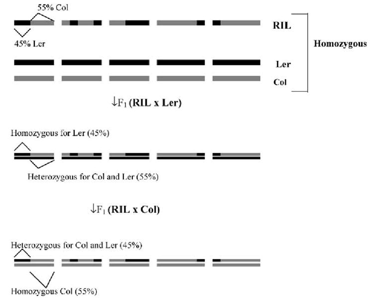
An ideogram showing genotype of homozygous RIL and the two parents, Col, Ler, and their F₁ hybrids that generate homozygosity/heterozygosity along exactly opposite regions between them and their proportion can be readily determined on each chromosome and entire genome from the published marker intervals.

The above measure of heterozygosity was then converted into weighted heterozygosity (WH) of each chromosome as follows:

WH = heterozygosity-per-chromosome×w_i

where w_i is the length of the chromosome as a proportion of the whole genome length. For example, chromosome 1 is 131.6cM long and the total genome length of A. thaliana is 579.13cM. So, w_i = 131.6/579.13=0.2272 and WH of chromosome 1 is 55 × 0.2272=12.50. Similarly, the WH of the remaining 45% on the same chromosome after crossing with the second parent is 45 × 0.2272 = 10.22. The total WH for this chromosome is 22.72 (12.50+10.22) with one weight unit = 5.79cM (131.6/22.72). Similarly, the WH was calculated for each cross/chromosome combination, and these values were averaged throughout the genome by combining the (RIL × Col and Ler) groups resulting in one weight unit = 5.86cM. The high- and low-performing crosses were separated and the mean WH was calculated for each group for all traits in five chromosomes and the whole genome. The WH values of the whole genome were estimated based on the total mean WH in a particular group for each trait.

Heterosis and regression analysis

Absolute MPH and relative mid-parent heterosis (RMPH) values were calculated following Barth et al (2003) as

$$\mathrm{MPH}=({\overline{F}}_1-\overline{P})/\overline{P}$$

$$\mathit{RMPH}=100\times ({\overline{F}}_1-\overline{P})/\overline{P}$$

Where ${\overline{F}}_1$ is the mean of a test cross family and $\overline{P}$ is its mid-parental value.

The pooling of test crosses for each trait, based on low and high performance, is informative but it does not provide the statistical confidence to predict a relationship between heterozygosity and MPH. To investigate the relationship between observed heterosis and heterozygosity, the MPH (Y) values were regressed against heterozygosity (X) across the whole genome and on individual chromosomes using linear and multiple regression, respectively. All regression analyses were performed using Minitab software version 12.2.

Results

NCIII experiment

The 16 traits measured in each individual plant are shown in Table 1. The measurement for each trait was taken on the same day for all of the plants, except for those traits that were recorded sequentially by the onset of phenotypes, such as flowering. Significant additive and dominance effects were detected for almost all the traits (Table 1). Furthermore, high values for the dominance ratio (√4VD/2VA) were detected for most of the traits, in particular plant height having values close to or more than 1, indicating the presence of overdominance (data not shown).

High F₁ hybrid performance in the test cross progenies

Complete data sets comprising the mean performance of each of the 52 RILs and their crosses with Col and Ler for RS36 and H45 are presented in Table 2a and b, respectively. It is evident from the mean performance of each RIL and its crosses with Col and Ler that a large number of crosses performed better than the mean of the corresponding parents. Interestingly, a number of crosses of RILs performed better even when crossed with either Col or Ler. This is very interesting (Figure 1) because a particular RIL when crossed with Col and Ler generates homozygosity and heterozygosity along exactly opposite regions. RMPH values were as high as 38 and 64% for RS36 and H45, respectively.

Table 2.

Mean values of indicated parents and crosses for the shown RILs (nos. as NASC) along with MPH and RMPH for each cross

(a) Rosette Size 36th day
RIL no.	RIL, mean	RIL × C, mean	RIL × L, mean	L1i P, mean	L2i P, mean	L1 MPH	L2 MPH	RMPH L1	RMPH L2
5	110.38	92.88	90.92	100.81	92.52	−7.94	−1.61	−7.87	−1.74
30	86.96	90.9	98.3	89.1	80.81	1.8	17.49	2.02	21.64
34	82.67	102.8	83.2	86.96	78.67	15.84	4.53	18.22	5.76
35	92.50	106.0	80.63	91.88	83.59	14.13	−2.96	15.37	−3.54
52	77.35	101.5	96.15	84.3	76.01	17.2	20.14	20.4	26.5
54	91.78	84.4	81.83	91.51	83.22	−7.11	−1.4	−7.77	−1.68
59	102.81	92.1	84.9	97.03	88.74	−4.93	−3.84	−5.08	−4.33
67	71.37	94.1	85.1	81.31	73.02	12.79	12.08	15.73	16.55
68	79.35	86.4	75.9	85.3	77.01	1.1	−1.11	1.29	−1.44
79	95.85	98.6	103.08	93.55	85.26	5.05	17.82	5.4	20.89
84	86.8	84.98	96.78	89.03	80.74	−4.05	16.04	−4.55	19.87
90	81.57	104.5	97.2	86.41	78.12	18.09	19.08	20.94	24.43
107	101.58	107.4	81.7	96.42	88.13	10.98	−6.43	11.39	−7.29
113	96.03	110.1	82.3	93.64	85.35	16.46	−3.05	17.58	−3.57
115	96.43	115.6	96.1	93.84	85.55	21.76	10.55	23.19	12.33
123	94.53	91.8	73.45	92.89	84.6	−1.09	−11.15	−1.17	−13.18
131	83.13	109.23	97.25	87.19	78.9	22.04	18.35	25.28	23.26
160	98.85	106.1	90.0	95.05	86.76	11.05	3.24	11.63	3.73
161	88.40	105.07	87.8	89.83	81.54	15.24	6.27	16.97	7.68
173	87.90	104	85.2	89.58	81.29	14.43	3.92	16.1	4.82
177	86.43	100.4	78.5	88.84	80.55	11.56	−2.05	13.01	−2.55
181	75.28	105.2	78.75	83.26	74.97	21.94	3.78	26.35	5.04
182	86.24	102.0	88.5	88.74	80.45	13.26	8.05	14.94	10.0
190	84.00	102.8	106.3	87.63	79.34	15.18	26.97	17.32	33.99
191	59.68	102.15	86.7	75.46	67.17	26.69	19.53	35.37	29.07
193	88.31	99.0	83.98	89.78	81.49	9.22	2.49	10.27	3.05
194	93.06	99.9	102.5	92.16	83.87	7.74	18.63	8.4	22.22
199	89.98	104.2	99.08	90.62	82.33	13.58	16.75	14.99	20.34
209	80.26	107.2	83.45	85.75	77.46	21.45	5.99	25.01	7.73
214	93.77	100.9	87.63	92.51	84.22	8.39	3.4	9.07	4.04
217	101.78	123.3	84.0	96.51	88.22	26.79	−4.22	27.76	−4.79
231	82.85	109.6	97.9	87.05	78.76	22.55	19.14	25.9	24.3
238	97.53	90.5	74.3	94.39	86.1	−3.89	−11.8	−4.12	−13.71
240	78.21	102.8	77.2	84.73	76.44	18.07	0.76	21.33	1.0
242	79.95	102.7	86.9	85.6	77.31	17.1	9.59	19.98	12.4
245	59.90	104.1	86.9	75.58	67.29	28.53	19.62	37.74	29.15
257	84.33	102.8	99.8	87.79	79.5	15.01	20.3	17.1	25.53
263	87.2	100.1	79.03	89.23	80.94	10.88	−1.9	12.19	−2.35
266	79.37	98.1	90.9	85.31	77.02	12.79	13.88	14.99	18.02
279	91.33	108.3	85.0	91.29	83.0	17.01	2.0	18.64	2.41
283	81.28	102.1	79.6	86.26	77.97	15.84	1.63	18.36	2.09
284	78.43	104.6	78.13	84.84	76.55	19.76	1.58	23.29	2.06
288	90.69	102.28	85.8	90.97	82.68	11.3	3.12	12.43	3.77
296	102.83	100.7	85.1	97.04	88.75	3.66	−3.65	3.77	−4.11
302	79.25	95.37	94.3	85.25	76.96	10.12	17.34	11.87	22.53
321	84.45	109.1	92.0	87.85	79.56	21.25	12.44	24.19	15.64
358	81.73	97.8	92.4	86.49	78.2	11.31	14.2	13.08	18.16
359	80.60	99.8	74.07	85.93	77.64	13.88	−3.57	16.15	−4.6
363	77.3	102.2	88.55	84.28	75.99	17.93	12.57	21.27	16.54
370	84.63	101.93	97.05	87.94	79.65	13.98	17.4	15.9	21.84
377	85.86	89.7	107.0	88.55	80.26	1.15	26.74	1.29	33.31
395	97.53	99.4	79.38	94.39	86.1	5.01	−6.72	5.31	−7.81
(b) Plant height 45th day
RIL no.	RIL, mean	RIL × C, mean	RIL × L, mean	L1i P, mean	L2i P, mean	L1 MPH	L2 MPH	RMPH L1	RMPH L2
5	342	361.38	392.67	365.5	303.75	−4.13	88.92	−1.13	29.27
30	320.58	378.9	458.2	354.79	293.04	24.11	165.16	6.8	56.36
34	358.0	384.6	291.1	373.5	311.75	11.1	−20.65	2.97	−6.62
35	313.33	396.9	262.75	351.17	289.42	45.73	−26.67	13.02	−9.21
52	278.25	408.63	294.93	333.63	271.88	75	23.05	22.48	8.48
54	315.08	398.5	340.7	352.04	290.29	46.46	50.41	13.2	17.37
59	406.16	419.2	284.45	397.58	335.83	21.62	−51.38	5.44	−15.3
67	275.06	372.5	318.8	332.03	270.28	40.47	48.52	12.19	17.95
68	271.2	420.4	297.9	330.1	268.35	90.3	29.55	27.36	11.01
79	399.23	375.6	431.3	394.11	332.36	−18.51	98.94	−4.7	29.77
84	268.73	323.05	370.5	328.86	267.11	−5.81	103.39	−1.77	38.71
90	274.3	424.2	413.8	331.65	269.9	92.55	143.9	27.91	53.32
107	324.25	387.8	311.5	356.63	294.88	31.18	16.63	8.74	5.64
113	335.46	403.7	261.68	362.23	300.48	41.47	−38.8	11.45	−12.91
115	309.17	390.5	421.3	349.08	287.33	41.42	133.97	11.86	46.62
123	431.85	397.0	303.6	410.43	348.68	−13.43	−45.08	−3.27	−12.93
131	309.4	400.03	373.45	349.2	287.45	50.83	86.0	14.55	29.92
160	388.98	381.65	309.08	388.99	327.24	−7.34	−18.16	−1.89	−5.55
161	312.04	393.27	307.5	350.52	288.77	42.75	18.73	12.19	6.49
173	302.95	451.3	330.73	345.98	284.23	105.33	46.5	30.44	16.36
177	389.57	401.6	276.9	389.28	327.53	12.32	−50.63	3.16	−15.46
181	280.83	458.0	263.5	334.92	273.17	123.08	−9.67	36.75	−3.54
182	320.88	399.0	292.1	354.94	293.19	44.06	−1.09	12.41	−0.37
190	355.25	425.0	466.8	372.13	310.38	52.88	156.43	14.21	50.4
191	199.68	369.9	283.1	294.34	232.59	75.56	50.51	25.67	21.72
193	250.24	424.5	312.6	319.62	257.87	104.88	54.73	32.81	21.22
194	292.19	426.0	457.1	340.59	278.84	85.41	178.26	25.08	63.93
199	316.34	364.5	404.37	352.67	290.92	11.83	113.45	3.35	39.0
209	286.8	373.6	277.25	337.9	276.15	35.7	1.1	10.57	0.4
214	379.89	405.9	328.5	384.45	322.7	21.45	5.8	5.58	1.8
217	361.75	470.4	314.0	375.38	313.63	95.03	0.38	25.31	0.12
231	262.95	410.2	423.1	325.98	264.23	84.23	158.88	25.84	60.13
238	300.29	359.3	295.3	344.65	282.9	14.65	12.4	4.25	4.38
240	274.43	411.9	290.2	331.72	269.97	80.18	20.23	24.17	7.49
242	256.43	382.7	279.5	322.72	260.97	59.98	18.53	18.59	7.1
245	233.38	372.9	268.6	311.19	249.44	61.71	19.16	19.83	7.68
257	306.7	383.9	406.95	347.85	286.1	36.05	120.85	10.36	42.24
263	321.83	403.0	325.05	355.42	293.67	47.58	31.38	13.39	10.69
266	335.97	396.2	341.7	362.49	300.74	33.71	40.96	9.3	13.62
279	319.33	397.17	292.1	354.16	292.41	43.0	−0.31	12.14	−0.11
283	244.85	396.9	277.6	316.93	255.18	79.98	22.43	25.23	8.79
284	239.18	412.3	317.95	314.09	252.34	98.21	65.61	31.27	26
288	299.48	395.93	304.7	344.24	282.49	51.68	22.21	15.01	7.86
296	320.25	423.38	338.9	354.63	292.88	68.75	46.03	19.39	15.71
302	295.48	373.73	364.2	342.24	280.49	31.5	83.71	9.2	29.85
321	283.2	409.2	305.8	336.1	274.35	73.1	31.45	21.75	11.46
358	258.63	399.4	355.8	323.81	262.06	75.59	93.74	23.34	35.77
359	324.9	428.3	283.7	356.95	295.2	71.35	−11.5	19.99	−3.9
363	265.35	416.15	290.03	327.18	265.43	88.98	24.6	27.19	9.27
370	302.11	414.88	384.6	345.55	283.8	69.32	100.8	20.06	35.52
377	250.53	353.3	412.4	319.77	258.02	33.53	154.38	10.49	59.83
395	331.83	387.0	259.5	360.41	298.66	26.59	−39.16	7.38	−13.11

L1i and L2i refer to crosses of RILs with Col and Ler, respectively, and L1 P and L2 P are means of RIL and Col and of RIL and Ler, respectively.

To have an overview of all the traits studied, Table 3 shows the mean and range values of Col, Ler and their F₁ hybrids as well as RIL × Col and RIL × Ler progenies for all traits. Col was the high-performing parent as it had higher scores than Ler for 12 out of the 16 traits. Indeed, higher values for the majority of traits were found in the crosses where Col was used as a maternal parent. However, for most traits except plant height, the differences between the reciprocal crosses were not statistically significant. In the RILs, the mean values for most of the traits examined were within the range of the two parents ruling out dominance complementation. Furthermore, the reciprocal hybrids of Col and Ler were also poor performing compared to test cross hybrids. In the test cross progeny (RILs × Col or Ler), the majority of lines displayed high F₁ hybrid performance for most of the 16 traits studied. The mean values of the RILs × Col progeny for almost all of the traits were higher than that of parental RILs and Col, except for a few crosses with low F₁ hybrid performance. The test cross progenies had higher mean values for many traits than individual RILs and reciprocal F₁ hybrids. The data indicate that total heterozygosity across the whole genome is not as important for phenotypic expression as heterozygosity of some specific tracts especially regions bearing QTLs (see below) for different traits. Furthermore, in the progeny of RIL × Col, the frequency of high- and low-performance lines for a particular trait was somewhat evenly distributed, whereas in the RIL × Ler progeny, the distribution of high- or low-performance lines was skewed. The data suggest that the effects of heterozygosity on hybrid performance are genotype dependent. Furthermore, the F₁ hybrid performance of the progenies of RILs × Col and RILs × Ler was higher than that in the RILs, suggesting that heterozygosity/overdominance and/or epistasis is one of the main factors for hybrid vigor.

Table 3.

Mean and range values for the two parents (Col and Ler) and their reciprocal crosses along with RILs and their test crosses with Col and Ler

Trait	Ler	Col	L × C	C × L	RILS		RILs × Col			RILs × Ler
	Mean	Mean	Mean	Mean	Mean	Range	Mean	High F1	Range	Mean	High F1s	Range
TL	14.85	11.8	13.0	12.0	12.39	11.5–13.6	12.02	34	11.1–13.9	12.38	51	11.1–14.5
RL26	7.77	10.45	8.33	9.53	9.72	8.5–11.9	9.93	22	8.8–11.5	9.18	42	7.6–10.9
RLFL	8.71	10.9	8.87	10.06	9.96	8.4–11.8	10.52	29	9.3–16.2	9.38	25	8.2–10.9
RS26	27.62	56.95	48.22	58.27	47.35	30.7–62.7	55.11	35	36.6–64.7	50.89	51	31.8–70.2
RS36	74.67	91.25	89.33	95.67	87.13	59.6–110.3	101.1	46	84.4–123.3	88.23	37	73.4–106.3
RSFL	68.14	75.26	70.88	76.87	66.33	46.2–88.2	76.10	43	66.3–94.4	67.23	26	53.9–83.9
CL26	1.66	5.61	4.89	5.93	4.19	0.92–10.1	4.68	25	0.85–9.3	5.29	46	0.35–10.7
CLFL	19.67	17.24	13.0	13.53	16.27	10.2–24	17.52	29	11.6–25.7	15.18	4	9.17–20.2
DF	32.11	28.5	26.8	28.46	29.14	27.3–32.4	28.91	27	26.5–33.3	28.70	48	27–31.45
BFL	10.42	11.55	8.25	9.8	10.41	8.7–12.1	10.45	17	8.7–12.9	9.75	9	7.7–12.2
HFL	37.14	46.18	52.55	58.13	35.54	19.5–56.6	50.65	46	31.3–70	38.51	26	22–65.8
H35	70.9	244.75	192.6	261.69	143.82	78.8–244.6	207.78	37	77.3–268.3	173.9	50	87.3–278.3
H45	265.5	389.0	384.3	431.9	308.95	199.6–431.8	399.25	47	323–470.4	333.38	40	261.6–466.8
LL45	42.67	46.7	50.56	49.93	46.96	31.1–56.7	54.22	48	46.5–62.8	47.42	32	38.6–57.7
Lw45	21.44	17.0	21.11	19.53	19.95	14.3–27.9	20.39	45	16.8–23.8	21.10	13	18.8–24.1
Ma	54.0	49.73	51.44	49.93	51.15	48.9–53.2	50.36	25	48.5–53	50.39	1	47.8–52.9

The numbers of high-performing F₁ hybrids over the mean of the parents are also indicated for each group.

QTL analysis

QTL cartographer, which is capable of performing CIM, was employed to map QTLs using RIL scores and additive and dominance components from the NCIII experiment, which allows us to compare the efficiency of the two methods, marker regression and CIM. The QTL analysis using the same population by marker regression approach (Kearsey and Hyne, 1994) has been reported elsewhere (Kearsey et al, 2003). The presence of QTLs was only indicated on individual chromosomes showing significant regressions of F₁ heterosis on heterozygosity in Tables 4 and 5 to determine that whether heterozygosity along chromosomes bearing QTLs is relatively more important.

Table 4.

Mean heterozygosity in cM in individual chromosomes as well as across the entire genome for (a) RILs × Col, (b) RILs × Ler groups for high- (shown in boldface) versus low-performing F_1s for the indicated traits

Trait	LG1 (131.60 cM)	LG2( 93.29 cM)	LG3 (97.68 cM)	LG4 (116.28 cM)	LG5 (140.28 cM)	Total (579.13 cM)
(a)
TL	54.7 (60.7)	63.4 (69.2)	47.4 (49.1)	50.7 (55.8)	83.0 (73.7)	299.3 (308.8)
RL26	64.3 (54.7)*	57.9 (73.5)**	46.5 (49.7)*	61.5 (48.9)	68.2 (82.3)	298.6 (309.5)
RLFL	62.1 (54.3)*	62.8 (72.7)	45.2 (52.6)	56.6 (50.8)	69.7 (85.3)*	296.5 (315.9)
RS26	62.4 (50.2)	73.5 (54.2)**	47.0 (51.7)	46.9 (68.8)*	68.9 (92.4)	298.8 (318.2)
RS36	62.3 (30.5)**	68.7 (55.9)**	47.7 (54.7)	54.6 (49.5)*	77.1 (72.6)	310.7 (263.4)
RSFL	61.1 (46.7)	67.4 (66.2)***	43.8 (60.8)	52.6 (60.8)	75.3 (82.7)	300.5 (317.4)
CL26	54.5 (62.8)*	70.3 (64.1)	50.7 (46.3)	47.8 (60.2)**	71.7 (81.5)	295.2 (315.0)
CLFL	66.9 (48.2)	68.7 (65.3)***	44.1 (54.0)	53.5 (54.7)*	74.9 (78.7)***	308.2 (301.2)
BFL	62.8 (50.1)	60.3 (81.4)	49.9 (45.5)	57.4 (47.2)	77.5 (74.7)**	308.1 (299.2)
DF	59.2 (58.1)	65.2 (69.0)	44.7 (52.1)	60.4 (48.2)**	85.1 (68.7)	314.8 (296.2)
HFL	61.2 (39.0)	68.8 (55.3)***	45.0 (75.5)	53.5 (58.6)	74.0 (96.9)**	302.5 (325.5)
H35	63.4 (46.8)***	72.7 (53.6)***	49.5 (46.0)	49.9 (64.2)	75.8 (78.5)	311.5 (289.3)
H45	62.4 (23.2)***	70.2 (38.9)***	47.0 (62.4)	50.8 (84.3)	74.0 (101.2)	304.6 (310.1)
LL45	59.7 (45.1)**	68.1 (56.3)**	49.6 (35.5)	56.3 (26.4)	78.9 (48.3)	312.9 (211.9)
LW45	58.9 (56.6)	66.6 (71.2)**	50.2 (37.3)	58.8 (23.0)	80.2 (53.2)**	315.0 (241.5)
Ma	65.9 (51.9)*	64.2 (70.0)	43.7 (52.9)*	62.9 (45.8)	78.8 (74.5)*	315.7 (295.4)
(b)
TL	73.7 (42.1)	31.1 (31.4)	53.2 (47.7)	62.2 (67.5)	61.3 (16.4)	281.8 (205.3)
RL26	72.2 (77.2)*	30.9 (32.4)**	58.3 (31.0)*	64.6 (52.9)	64.4 (44.1)	290.6 (237.7)
RLFL	70.1 (76.2)*	32.3 (30.3)	51.3 (54.9)	62.2 (62.5)	69.3 (51.5)*	285.5 (275.3)
RS26	74.1 (23.7)	31.8 (0.00)**	52.9 (63.0)	62.5 (53.5)*	61.5 (4.10)	283.0 (144.4)
RS36	75.4 (67.6)**	31.3 (30.8)**	55.2 (48.0)	58.1 (73.0)*	61.5 (57.7)	281.6 (277.3)
RSFL	74.8 (71.6)	38.2 (24.7)***	56.1 (50.3)	62.8 (62.0)	68.3 (53.1)	300.5 (261.8)
CL26	74.4 (63.0)*	31.4 (29.0)	55.0 (38.15)	59.7 (83.3)**	62.1 (47.5)	282.9 (261.0)
CLFL	71.8 (73.3)	38.6 (30.5)***	59.4 (52.6)	77.7 (61.1)*	69.6 (59.7)***	317.3 (277.3)
BFL	73.5 (73.0)	12.7 (35.0)	62.2 (51.2)	67.8 (61.3)	79.9 (56.4)**	296.4 (277.0)
DF	59.6 (74.3)	13.2 (23.7)	43.1 (53.9)	79.2 (60.9)**	52.4 (61.1)	247.7 (283.1)
HFL	77.2 (69.0)	44.0 (18.4)***	52.3 (53.9)	66.8 (58.0)	63.8 (57.1)**	304.3 (256.5)
H35	73.8 (56.0)***	32.4 (0.94)***	53.4 (45.2)	61.5 (83.9)	61.8 (26.7)	283.1 (212.8
H45	72.2 (76.3)***	33.4 (23.7)***	60.7 (27.7)	59.4 (72.1)	62.6 (53.2)	288.4 (253.3)
LL45	76.4 (67.5)**	34.1 (26.0)**	54.2 (51.2)	61.8 (63.4)	63.9 (54.5)	290.5 (262.7)
LW45	57.4 (78.4)	34.7 (30.0)**	56.1 (52.1)	65.2 (61.4)	55.6 (62.1)**	269.2 (284.0)
Ma	23.7 (74.1)*	0.0 (31.8)	63.0 (52.2)*	53.5 (62.5)	4.1 (61.5)*	144.4 (283.0)

*, ** and *** indicate the presence of a QTL beyond 0.05, 0.01 and 0.001 probability levels, respectively.

Table 5.

Significant regression coefficients with their standard deviation (SD) values of the test cross scores on total marker heterozygosity (a) and on individual chromosomes marker heterozygosity (b) for the indicated traits and crosses

(a)
Trait	RILs × Ler (b ± SD)		RILs × Col (b ± SD)		High parent (P)
TL	0.015 ± 0.007		—		Ler
RLFL	0.011 ± 0.005		—		Col
RS26	0.193 ± 0.072		—		Col
RSFL	0.156 ± 0.078		—		Col
HFL	0.362 ± 0.149		—		Col
H35	1.077 ± 0.385		—		Col
H45	—		0.62 ± 0.286		Col
(b)
Trait	Cross	Chr1 (b ± SD)	Chr2 (b ± SD)	Chr3 (b ± SD)	Chr4 (b ± SD)	Chr5 (b ± SD)
RL26	RILs × Col	—	0.041 ± 0.02*	—	—	—
RLFL	RILs × Ler	—	—	—	—	0.028 ± 0.011
RS26	RILs × Ler	—	0.537 ± 0.020*	—	—	—
RS36	RILs × Ler	—	0.643 ± 0.281*	—	—	—
RSFL	RILs × Ler	—	0.833 ± 0.206*	—	—	—
CL26	RILs × Col	—	—	—	0.129 ± 0.052*	—
DF	RILs × Col	—	—	—	0.071 ± 0.034*	—
	RILs × Ler	0.052 ± 0.024	—	—	—	—
BFL	RILs × Col	—	—	0.065 ± 0.033	—	—
HFL	RILs × Col	—	0.721 ± 0.290*	—	—	—
	RILs × Ler	—	1.758 ± 0.384*	—	—	—
H35	RILs × Col	—	2.447 ± 1.213*	—	—	—
	RILs × Ler	—	3.982 ± 1.047*	—	—	—
H45	RILs × Col	—	1.773 ± 1.495*	—	—	—
	RILs × Ler	—	5.848 ± 1.495*	—	—	—
LL45	RILs × Ler	—	0.507 ± 0.137*	—	—	—
LW45	RILs × Col	—	—	—	—	0.094 ± 0.038
	RILs × Ler	—	0.091 ± 0.043*	—	—	—
Ma	RILs × Ler	0.081 ± 0.03*	—	—	—	—

R²-values, which are between 15 and 20%, are not shown.

^*indicates the presence of a QTL on a particular chromosome.

Distribution of Col and Ler regions in the RIL population

We estimated the proportion (percentage) of Col and Ler genotype (marker intervals) regions among the selected RILs. Interestingly, each RIL used in this study had approximately 51% of the genome from Col and 49% of that from Ler in the marker genotypes analyzed in each of the five chromosomes (data not shown). Ideally, the proportion should be 50–50. Indeed, χ²-test showed that it is not significantly different from a 1:1 ratio, suggesting that the original population of RILs derived from the two parents represented a random sample of lines through single-seed descent, hence exhibiting a random distribution of recombination events for each parent. However, individual RILs had significant differences in Col and Ler regions in their genotypes and heterozygosity generated in crosses with the two parents, Col and Ler.

RILs × Col crosses

The weight of heterozygosity on each chromosome was estimated for all the RILs showing positive high F₁ hybrid performance for each trait. The total (mean) weight of heterozygosity in each chromosome was then transformed into cM by multiplying with 5.86 (see Materials and methods). The difference in total heterozygosity between low- and high-performing crosses for the majority of traits, except LL45 and LW 45, is relatively small. Heterozygosity levels in individual chromosomes of the high-performing crosses for traits RS36, CLFL, DF, BFL, H35, LL45, LW45 and Ma (Table 4) were slightly higher than that of low-performing crosses, indicating that heterozygosity in individual chromosomes bearing QTLs was more important than the total heterozygosity. In most cases (Table 4), the chromosomes bearing QTLs had a much higher level of heterozygosity in the high-performing crosses than in the low-performing crosses. For example, the mean heterozygosity for RS26, H35, HFL and H45 in better-performing pooled crosses was much higher than in the low-performing crosses. However, for many other traits, such as RSFL, CLFL and BFL, there was no significant difference in mean heterozygosity between the high- and low-performing pooled crosses. Furthermore, the highest heterozygosity in a chromosomal region is not necessarily associated with a QTL. The highest mean heterozygosity (pooled crosses) for H45 was found in chromosome 5; however, two QTLs for H45 were located in chromosomes 1 and 2 (data not shown).

RILs × Ler crosses

The RILs × Ler crosses exhibited patterns of phenotypic variation similar to that of RILs × Col crosses (Tables 2 and 3). After pooling high- and low-performing crosses for each trait, 13 out of the 16 traits showed high levels in total heterozygosity (in cM). In general, the difference in total heterozygosity between high- and low-performing crosses in RILs × Ler hybrids was higher than that in RILs × Col hybrids. Within the RILs × Ler lines, the difference between low- and high-performing crosses can be as high as 139 cM (eg for RS26). High-performing RILs × Ler hybrids had much higher levels of heterozygosity than the low-performing crosses in individual chromosomes. For example, chromosomes bearing QTLs for RLFL, RS26, CLFL, BFL, HFL and H45 had higher levels of heterozygosity in high-performing than low-performing F₁s. This difference in RILs × Ler hybrids was much larger than in RILs × Col hybrids.

F₁ performance and marker heterozygosity

To evaluate our pooling method and estimates for marker heterozygosity, total heterozygosity as well as heterozygosity along individual chromosomes was regressed against MPH values of all traits in RILs × Col and RILs × Ler crosses. Linear regression analysis suggests that the test cross performance is significantly associated with overall marker heterozygosity for several traits (Table 5a). In the RILs × Col progeny only H45 was significantly associated with total marker heterozygosity, whereas in the RILs × Ler progeny significant regression was detected for TL, RS26, RLFL, RSFL, HFL and H35, respectively. The data suggest that the hybrid performance is dependent on marker heterozygosity in some of the traits studied. However, R²-values were relatively small, ranging from 15 to 20% indicating that that only a small proportion of the observed heterosis is directly explained by heterozygosity and that some other factors are involved.

To have a better understanding of the relationship between marker heterozygosity and hybrid performance, we further performed multiple linear regression analysis using MPH values and marker heterozygosity on individual chromosomes (Table 5b). The hybrid performance in the test cross progenies was significantly associated with marker heterozygosity in most chromosomes (Tables 4 and 5). Elimination of nonsignificant regressions from the multiple regression analysis did not make much difference and the outcome essentially remained the same (data not shown). The number of traits with significant regression to marker heterozygosity was not evenly distributed among five chromosomes. Out of 19 trait/chromosome combinations in chromosome 2, 12 showed significant regression with marker heterozygosity. The number of traits in other chromosomes were low: two, one, two and two for chromosomes 1, 3, 4 and 5, respectively. It is notable that each of the 17 significant regressions of traits and marker heterozygosity in individual chromosomes was associated with one or more QTLs. This indicates that marker heterozygosity in individual chromosomes and especially in the QTL regions is more important for phenotypic variation than the total heterozygosity in the genome.

Discussion

A. thaliana Col and Ler ecotypes share similar genetic backgrounds (King et al, 1993) and, indeed, the performance of RILs for most of the traits examined remained within mean values of the two parents (Col and Ler) ruling out dominance complementation for the majority of traits. However, we observed a large amount of variation in the F₁ (or backcross) hybrids derived from each of the RILs and its parent, Col or Ler. These F₁ lines showed low and high performance for all of the traits studied (Tables 2 and 3). It is notable that high F₁ performance was observed in F₁ lines derived from RILs × Col or Ler. The reciprocal hybrids between Col and Ler did not show a comparable superiority over the two parents. Moreover, total heterozygosity is not as important as heterozygosity in individual chromosomes or segments for the observed heterosis. The data suggest that differential heterozygosity combined with epistasis may be the reason for the observed heterosis. Epistasis was indeed found for TL, RL26, RS26, CL26, DF, H35, H45, LL45 and Ma in this population (Kearsey et al, 2003).

To test the hypothesis of maximum heterozygosity for high F₁ performance (Bonierbale et al, 1993), we divided all crosses into four groups: RILs × Col (low and high F₁ hybrid performance) and RILs × Ler (low and high F₁ hybrid performance) for all traits. The proportion of heterozygosity was estimated in each linkage group. Significant QTLs were mapped for 13 out of the 16 traits examined in the RIL population using CIM (Basten et al, 2001). In the RILs × Col backcross progeny, there was no significant difference between low- and high-performing lines; however, heterozygosity on individual chromosomes bearing QTLs was associated with high-performing lines. In the RILs × Ler lines, both total heterozygosity and heterozygosity in individual chromosomes were significantly associated with high-performing lines. Ler is the low-performing parent; therefore, lines having a greater proportion of homozygous Ler background are likely to perform poorly. When the RILs are crossed to the high-performing Col, the heterozygosity in these regions likely contributes to high performance. However, a large number of RILs, when they are crossed to either Col or Ler, show high F₁ hybrid performance (Table 2a and b). This looks intriguing because homozygous Col regions in RIL × Col become heterozygous in RIL × Ler, when the same RIL is used. Similarly, heterozygous Ler regions in RIL × Col become homozygous in RIL × Ler, therefore producing heterozygosity in exactly the opposite regions in two of the test crosses nonetheless giving rise to similar high F₁ hybrid performance. This may be due to classically duplicate dominant genes (when the dominant genes at two different loci (homozygous dominant or heterozygous) each produce the same phenotype without a cumulative effect) (Kearsey and Pooni, 1996).

We used linear and multiple linear regression analysis to further explore the relationship between total heterozygosity or heterozygosity in individual chromosomes and the observed F₁ hybrid performance (MPH). The regression analysis confirmed the conclusions obtained by pooling high- and low-performing lines for each trait. The total heterozygosity is not very important in hybrid performance among RILs × Col crosses; only the regression for H45 is significant. However, in RILs × Ler crosses, F₁ hybrid performance is dependent on total heterozygosity as well as heterozygosity on individual chromosomes and especially the ones bearing QTLs. However, small R²-values (15–20%) for the significant regression show that this relationship is not straightforward because other factors including epistasis, background effects and the origin of plant material may be involved. Heterozygosity may play an important role in the high F₁ performance as the dominance ratio for plant height from the NCIII experiment is close to, or more than, 1 (data not shown). Although Ler is a low-performing parent, a large proportion of RILs × Ler crosses shows higher performance than RILs × Col crosses (Tables 2 and 3). This may be explained by the homozygous Ler background in RILs × Ler lines, where the effect of the erecta mutation in the second chromosome on plant height is known to have higher penetrance (Torii et al, 1996). Therefore, the background effects, new gene combinations and epistatic complexes play a significant role in hybrid performance (Doebley et al, 1995; Rasmusson and Phillips, 1997).

The high F₁ performance observed for all traits in general and plant heights in particular results from the effects on different genetic backgrounds. Alleles in different backgrounds give rise to a different expression pattern for a particular trait. Thus, hybridization among such populations produces new combinations and generates novel variation, even though few phenotypic differences exist between the populations (Doebley et al, 1997). Plant height in Ler is affected by a single mutation, which makes it shorter than Col, which is taller and more spreading (Lister and Dean, 1993). The RILs × Ler lines showing low F₁ hybrid performance for traits HFL and H45 are homozygous at the erecta locus (data not shown). It is notable that homozygous Ler loci in RILs remain homozygous even in RIL × Ler lines. The erecta locus contributes to a certain plant height (Ler phenotype) in homozygous RILs. However, the erecta effect on plant height reduction is greatly enhanced in RILs × Ler lines. Although the erecta locus remains homozygous in RIL × Ler lines, its negative effect on plant height increases in a different genetic background, suggesting a trans-effect of heterozygosity on plant height in other regions of chromosomes. This finding is reminiscent of results obtained by Doebley et al (1995), which indicates that two QTLs affecting plant architecture and inflorescence structure have tremendously different effects in a maize or teosinte (wild progenitor of maize) background. The importance of genetic background effects and epistatic relationships among new combination of genes has been documented (Matzke et al, 1993; Pooni et al, 1994; Cheverud and Routman, 1995; Doebley et al, 1995; Cheverud and Routman, 1996; Eshed and Zamir, 1996; Routman and Cheverud, 1997).

Our results may also have implication for issues related to introduction of genetic diversity into plant breeding pursuits. Rasmusson and Phillips (1997) argued that the genetic gap between elite gene pools and unimproved pools or germplasm collections is growing larger with each breeding cycle (Martin et al, 1991). Introgression of genetic diversity from unimproved collections is becoming more difficult. They further argued that selection gains occur due to variation present in the original gene pool as well as de novo variation and this variation is augmented by epistasis, that is, interactions involving newly created diversity as well as original diversity. Such hypotheses stem from observations (eg Sprague et al, 1960; Russell et al, 1963) that doubled haploid lines of maize soon accumulated considerable variation in agronomic traits. Such variation for lines homozygous at every locus could not be expected due to occasional mutations. Rasmusson and Phillips (1997) reviewed the contribution of various events, such as intragenic recombination, unequal crossing over, transposable elements, DNA methylation, paramutation and gene amplification, to genome plasticity coupled with epigenetic modifications, base alterations and structural changes augmented by epistasis. Many authors have indicated the importance of epistasis and background genotype in creating novel variation and have emphasized that epistatic interactions are much more important than previously realized (Matzke et al, 1993; Doebley et al, 1995; Cheverud and Routman, 1995, 1996; Routman and Cheverud, 1997; Eshed and Zamir, 1996).

The results obtained from two closely related ecotypes in the model plant Arabidopsis may be applied to the improvement of genetic diversity in major crop plants, although further testing and experimentation will be needed in other plant and crop species. The results may be relevant to the growing genetic distance between elite crop varieties and exotic germplasm. In cases where very little variation exists for further improvement, similar schemes of crossing might be used to generate novel variation. Further work should also investigate the performance of F2 and F3 families of heterotic crosses, in particular the extent to which heterosis tends to dissipate in these generations due to loss of heterozygosity and gene combinations (Fenster and Galloway, 2000). The RIL population developed will be useful to dissect the molecular basis of dominance and overdominance (Birchler et al, 2003) using functional genomic tools such as genome-wide gene expression analysis using oligo-gene microarrays.

References

- 1.Barth S, Busimi AK, Friedrich Utz H, Melchinger AE. Heterosis for biomass yield and related traits in five hybrids of Arabidopsis thaliana L. Heynh. Heredity. 2003;91:36–42. doi: 10.1038/sj.hdy.6800276. [DOI] [PubMed] [Google Scholar]
- 2.Basten CJ, Weir BS, Zeng ZB. Statistics. North Carolina State University; Raleigh, NC: 2001. QTL cartographer version 1.15. [Google Scholar]
- 3.Bell CJ, Ecker JR. Assignment of 30 microsatellite loci to the linkage map of Arabidopsis. Genomics. 1994;19:137–144. doi: 10.1006/geno.1994.1023. [DOI] [PubMed] [Google Scholar]
- 4.Birchler JA, Augar DL, Riddle NC. In search of the molecular basis of heterosis. Plant Cell. 2003;15:2236–2239. doi: 10.1105/tpc.151030. [DOI] [PMC free article] [PubMed] [Google Scholar]
- 5.Bonierbale MW, Plaisted RL, Tanksley SD. A test of the maximum heterozygosity hypothesis using molecular markers in tetraploid potatoes. Theor Appl Genet. 1993;86:481–491. doi: 10.1007/BF00838564. [DOI] [PubMed] [Google Scholar]
- 6.Boppenmaier J, Melchinger AE, Seitz G, Geiger HH, Herrmann RG. Genetic diversity for RFLPs in Euporean maize inbreds III. Performance of crosses within versus between heterotic groups for grain traits. Plant Breed. 1993;111:217–226. [Google Scholar]
- 7.Bruce AB. The Mendelian theory of heredity and the augmentation of vigor. Science. 1910;32:627–628. doi: 10.1126/science.32.827.627-a. [DOI] [PubMed] [Google Scholar]
- 8.Cheverud JM, Routman EJ. Epistasis and its contribution to genetic variance components. Genetics. 1995;139:1455–1461. doi: 10.1093/genetics/139.3.1455. [DOI] [PMC free article] [PubMed] [Google Scholar]
- 9.Cheverud JM, Routman EJ. Epistasis as source of increased additive genetic variance at population bottlenecks. Evolution. 1996;50:1042–1051. doi: 10.1111/j.1558-5646.1996.tb02345.x. [DOI] [PubMed] [Google Scholar]
- 10.Cockerham CC, Zeng ZB. Design III with marker loci. Genetics. 1996;143:1437–1456. doi: 10.1093/genetics/143.3.1437. [DOI] [PMC free article] [PubMed] [Google Scholar]
- 11.Comstock RE, Robinson HF. In: Heterosis. Gowen JW, editor. Iowa State College Press; Ames, IA: 1952. pp. 494–516. [Google Scholar]
- 12.Coors JG, Pandey S, editors. Genetics and Exploitation of Heterosis in Crops. American Society of Agronomy Inc.; Madison, WI: 1999. [Google Scholar]
- 13.Crow JF. Alternative hypothesis of hybrid vigor. Genetics. 1948;33:477–487. doi: 10.1093/genetics/33.5.477. [DOI] [PMC free article] [PubMed] [Google Scholar]
- 14.Dobzhansky T. Genetics of natural populations. XIX. Origin of heterosis through natural selection in populations Drosophila pseudobscura. Genetics. 1950;35:288–302. doi: 10.1093/genetics/35.3.288. [DOI] [PMC free article] [PubMed] [Google Scholar]
- 15.Doebley J, Stec A, Gustus C. Teosinte branched1 and the origin of maize: evidence for epistasis and the evolution of dominance. Genetics. 1995;141:333–346. doi: 10.1093/genetics/141.1.333. [DOI] [PMC free article] [PubMed] [Google Scholar]
- 16.Doebley J, Stec A, Hubbard L. The evolution of apical dominance in maize. Nature. 1997;386:485–488. doi: 10.1038/386485a0. [DOI] [PubMed] [Google Scholar]
- 17.Dudley JW, Saghai Maroof MA, Rufener GK. Molecular markers and grouping of parents in maize breeding programmes. Crop Sci. 1991;31:718–723. [Google Scholar]
- 18.East EM. Heterosis. Genetics. 1936;21:375–397. doi: 10.1093/genetics/21.4.375. [DOI] [PMC free article] [PubMed] [Google Scholar]
- 19.Eshed Y, Zamir D. Less-than-additive epistatic interactions of quantitative trait loci in tomato. Genetics. 1996;143:1807–1817. doi: 10.1093/genetics/143.4.1807. [DOI] [PMC free article] [PubMed] [Google Scholar]
- 20.Fenster CB, Galloway LF. Population differentiation in an annual legume genetic architecture. Evolution. 2000;54:1157–1172. doi: 10.1111/j.0014-3820.2000.tb00551.x. [DOI] [PubMed] [Google Scholar]
- 21.Godshalk EB, Lee M, Lamkey KR. Relationship of restriction fragment length polymorphism to single-cross hybrid performance of maize. Theor Appl Genet. 1990;80:273–280. doi: 10.1007/BF00224398. [DOI] [PubMed] [Google Scholar]
- 22.Jinks JL. A survey of the genetical basis of heterosis in a variety of diallel crosses. Heredity. 1955;9:223–238. [Google Scholar]
- 23.Jones DF. Dominance of linked factors as a means of accounting for heterosis. Genetics. 1917;2:466–479. doi: 10.1093/genetics/2.5.466. [DOI] [PMC free article] [PubMed] [Google Scholar]
- 24.Kearsey MJ, Hyne V. QTL analysis: a simple ‘marker regression approach’. Theor Appl Genet. 1994;89:698–702. doi: 10.1007/BF00223708. [DOI] [PubMed] [Google Scholar]
- 25.Kearsey MJ, Pooni HS. The Genetical Analysis of Quantitative Traits. Chapman and Hall; London: 1996. [Google Scholar]
- 26.Kearsey MJ, Pooni HS, Syed NH. The genetics of quantitative traits in Arabidopsis thaliana. Heredity. 2003;91:456–464. doi: 10.1038/sj.hdy.6800306. [DOI] [PubMed] [Google Scholar]
- 27.King G, Nienhuis J, Hussey C. Genetic similarity among ecotypes of Arabidopsis thaliana estimated by analysis of restriction fragment length polymorphism. Theor Appl Genet. 1993;86:1028–1032. doi: 10.1007/BF00211057. [DOI] [PubMed] [Google Scholar]
- 28.Lee M, Godshalk EB, Lamkey KR, Woodman WW. Association of restriction fragment length polymorphisms among maize inbreds with agronomic performance of their crosses. Crop Sci. 1989;30:1033–1040. [Google Scholar]
- 29.Li ZK, Luo LJ, Mei HW, Wang DL, Shu QY, Tabien R, et al. Overdominant epistatic loci are the primary genetic basis of inbreeding depression and heterosis in rice. I. Biomass and grain yield. Genetics. 2001;158:1737–1753. doi: 10.1093/genetics/158.4.1737. [DOI] [PMC free article] [PubMed] [Google Scholar]
- 30.Lister C, Dean C. Recombinant inbred lines for mapping RFLP and phenotypic markers in Arabidopsis thaliana. Plant J. 1993;4:745–750. doi: 10.1046/j.1365-313x.1996.10040733.x. [DOI] [PubMed] [Google Scholar]
- 31.Luo LJ, Li ZK, Mei HW, Shu QY, Tabien R, Zhong DB, et al. Overdominant epistatic loci are the primary genetic basis of inbreeding depression and heterosis in rice. II. Grain yield components. Genetics. 2001;158:1755–1771. doi: 10.1093/genetics/158.4.1755. [DOI] [PMC free article] [PubMed] [Google Scholar]
- 32.Martin JM, Blake TK, Hockett EA. Diversity among North American spring barley cultivars based on coefficients of parentage. Crop Sci. 1991;31:1131–1137. [Google Scholar]
- 33.Matzke JM, Neuhuber F, Matzke AJM. A variety of epistatic interactions can occur between partially homologous transgene loci brought together by sexual crossing. Mol Gen Genet. 1993;236:379–386. doi: 10.1007/BF00277137. [DOI] [PubMed] [Google Scholar]
- 34.Melchinger AE, Lee M, Lamkey KR, Woodman WL. Genetic diversity for restriction fragment length polymorphisms: relation to estimated genetic effects in maize inbreds. Crop Sci. 1990;30:1033–1040. doi: 10.1007/BF00226750. [DOI] [PubMed] [Google Scholar]
- 35.Mitchell-Olds T. Interval mapping of viability loci causing heterosis in Arabidopsis. Genetics. 1995;140:1105–1109. doi: 10.1093/genetics/140.3.1105. [DOI] [PMC free article] [PubMed] [Google Scholar]
- 36.Pooni HS, Virk PS, Coombs DT, Chowdhury MKU. The genetic basis of hybrid vigor in highly heterotic cross of Nicotiana tabacum. Theor Appl Genet. 1994;89:1027–1031. doi: 10.1007/BF00224534. [DOI] [PubMed] [Google Scholar]
- 37.Rasmusson DC, Phillips RL. Plant breeding progress and genetic diversity from de novo variation and elevated epistasis. Crop Sci. 1997;37:303–310. [Google Scholar]
- 38.Routman EJ, Cheverud JM. Gene effects on a quantitative trait: two locus epistatic effects measured at microsatellite markers and estimated QTL. Evolution. 1997;51:1654–1662. doi: 10.1111/j.1558-5646.1997.tb01488.x. [DOI] [PubMed] [Google Scholar]
- 39.Russell WA, Sprague GF, Penny LH. Mutations affecting quantitative characters in long time inbred lines of maize. Crop Sci. 1963;3:175–178. [Google Scholar]
- 40.Shull GH. The composition of a field of maize. Am Breeders Assoc Rep. 1908;4:296–301. [Google Scholar]
- 41.Smith OS, Smith JSC, Brown SL, Tenborg RA, Wall SJ. Similarities among a group of elite maize inbreds as measured by pedigree, F1 grain yield, grain yield heterosis and RFLPs. Theor Appl Genet. 1990;80:833–840. doi: 10.1007/BF00224201. [DOI] [PubMed] [Google Scholar]
- 42.Sprague GF, Russell WA, Penny LH. Mutations affecting quantitative traits in selfed progeny of doubled monoploid maize stocks. Genetics. 1960;45:855–865. doi: 10.1093/genetics/45.7.855. [DOI] [PMC free article] [PubMed] [Google Scholar]
- 43.Stuber CW, Lincoln SE, Wolff DW, Helentjaris T, Lander ES. Identification of genetic factors contributing to heterosis in a hybrid from two elite maize inbred lines using molecular markers. Genetics. 1992;132:823–839. doi: 10.1093/genetics/132.3.823. [DOI] [PMC free article] [PubMed] [Google Scholar]
- 44.Torii KU, Mitsukawa N, Oosumi T, Matsuura Y, Yokoyama R, Whittier RF, et al. The Arabidopsis ERECTA gene encodes a putative receptor protein kinase with extracellular leucine-rich repeats. Plant Cell. 1996;8:735–746. doi: 10.1105/tpc.8.4.735. [DOI] [PMC free article] [PubMed] [Google Scholar]
- 45.Virk PS, Pooni HS, Syed NH, Kearsey MJ. Fast and reliable genotype validation using microsatellite markers in Arabidopsis thaliana. Theor Appl Genet. 1999;98:462–464. [Google Scholar]
- 46.Xiao J, Li J, Yuan L, Tanksley SD. Dominance is the major genetic basis of heterosis in rice as revealed by QTL analysis using molecular markers. Genetics. 1995;140:745–754. doi: 10.1093/genetics/140.2.745. [DOI] [PMC free article] [PubMed] [Google Scholar]
- 47.Zeng ZB. Theoretical basis for separation of multiple linked gene effects in mapping quantitative trait loci. Proc Natl Acad Sci USA. 1993;90:10972–10976. doi: 10.1073/pnas.90.23.10972. [DOI] [PMC free article] [PubMed] [Google Scholar]