Measurement of Kinetic Parameters in Skeletal Muscle by Magnetic Resonance Imaging With an Intravascular Agent

Abstract

The purpose of this work was to investigate the use of an intravascular contrast agent to determine perfusion kinetics in skeletal muscle. A two-compartment kinetic model was used to represent the flux of contrast agent between the intravascular space and extravascular extracellular space (EES). The relationship between the image signal-to-noise ratio (SNR) and errors in estimating permeability surface area product (K^trans), interstitial volume (v_e), and plasma volume (v_p) for linear and nonlinear curve-fitting methods was estimated from Monte Carlo simulations. Similar results were obtained for both methods. For an image SNR of 60, the estimated errors in these parameters were 10%, 22%, and 17%, respectively. In vivo experiments were conducted in rabbits to examine physiological differences between these parameters in the soleus (SOL) and tibialis anterior (TA) muscles in the hind limb. Values for K^trans were significantly higher in the SOL (3.2 ± 0.9 vs. 2.0 ± 0.5 × 10⁻³ min⁻¹), as were values for v_p (3.4 ± 0.8 vs. 2.1 ± 0.7%). Differences in v_e for the two muscles (8.7 ± 2.2 vs. 8.5 ± 1.6%) were not found to be significant. These results demonstrate that relevant physiological metrics can be calculated in skeletal muscle using MRI with an intravascular contrast agent.

Contrast-enhanced magnetic resonance imaging (CEMRI) has been shown to be a valuable diagnostic tool for evaluating physiological tissue parameters in the brain (1,2), myocardium (3), and tumors (4,5). In the context of ischemic injury to either the brain or myocardium, CEMRI can be used to evaluate the extent and severity of injury, as well as response to treatment. CEMRI has also been used to characterize tumor vasculature, which correlates with invasive and metastatic potential (6). The majority of MRI contrast agents distribute into the vascular space and extravascular extracellular space (EES), and are excluded from the intracellular space. The kinetics can therefore be described using a two-compartment model, as detailed by Tofts (7). Quantitative T₁ maps are used to estimate the contrast agent concentration in the vascular and EES compartments over time, and the Tofts model is used to extract physiological parameters from these time courses. Most studies have focused on the kinetics of FDA-approved extravascular agents, such as Gd-DTPA (e.g., Magnevist^™). These agents are small enough in size (∼0.5 kDa) to allow rapid extravasation from the vascular space into the interstitium. Delivery of these agents is usually flow-limited, however, which makes them ill-suited for studying changes in vascular permeability.

Intravascular MRI contrast agents are actively being studied for many clinical applications. These agents distribute primarily in the intravascular space, and may gradually extravasate into the EES under certain conditions. The dynamics, therefore, are relatively slow compared to an extravascular agent, which makes the delivery permeability- rather than flow-limited. Intravascular agents have been used extensively to study the vascular volume and vessel permeability in tumors (5,8,9), but have had limited use in the context of skeletal (10) or myocardial (11,12) muscle. One advantage of macromolecular agents is that they are sensitive to changes in capillary permeability and thus may have application in the identification of reperfusion injury (13) or the recognition of angiogenic neovasculature (14). Because of the limited distribution volume of intravascular agents, the contrast-to-noise ratio (CNR) is lower than that obtained with extravascular agents. The goal of this work was to investigate the feasibility of using an intravascular agent in conjunction with the Tofts two-compartment model with parameters that are typical for skeletal muscle. Computer simulations were used to evaluate the expected errors in parameter estimation using the Tofts model for a range of signal-to-noise ratios (SNRs) and parameter values. Experiments were conducted in rabbits to assess the volume transfer constant (K^trans), fractional interstitial volume (v_e), and fractional plasma volume (v_p) in the soleus (SOL) and tibialis anterior (TA) muscles in the lower limb. These two muscle groups were chosen to determine how the physiological differences between the “slow-twitch” SOL and “fast-twitch” TA are reflected in the Tofts parameters.

MATERIALS AND METHODS

Contrast Agent

Gadomer (Schering AG, Berlin, Germany) is a gadolinium (Gd)-based synthetic macromolecular contrast agent that remains primarily in the intravascular space. Each molecule is comprised of 24 Gd ions chelated with lysine residues to a central core. Gadomer has a molecular weight of about 17 kDa, but because of its shape it has a larger apparent molecular weight of 30–35 kDa. This higher apparent molecular weight ensures that the agent will remain primarily in the vascular space, with a small amount of extravasation into the interstitium, and at the same time the molecule will be small enough to enable fairly rapid renal clearance (15).

Pharmacokinetic Model

Given that Gadomer distributes primarily to the intravascular space, and to a lesser degree the EES (also called the interstitial space or interstitium), with exclusion from the intracellular space, a two-compartment model can be used to model the distribution and transport of the agent across the vessel endothelium, as shown in Fig. 1 (7,16). The plasma volume fraction of the intravascular compartment is denoted by v_p, and the EES volume fraction is denoted by v_e. The transfer constant from the vascular compartment to the EES is denoted by K^trans, and the rate constant for the reflux from the interstitium back to the vascular compartment is given by k_ep. The relationship between these two rate constants is given by:

$$k_{\mathrm{ep}}=K^{\mathrm{trans}}∕v_{\mathrm{e}}$$ [1]

The tissue concentration (C_t) of the agent is a weighted sum of the concentrations in the EES (C_e) and the plasma space (C_p):

$$C_{\mathrm{t}}=v_{\mathrm{e}}{C}_{\mathrm{e}}+v_{\mathrm{p}}{C}_{\mathrm{p}}$$ [2]

The differential equation and corresponding solution for the agent concentration in the EES are:

$$\frac{{\mathit{dC}}_{\mathrm{e}}}{\mathit{dt}}=k_{\mathrm{ep}}(C_{\mathrm{p}}-C_{\mathrm{e}})$$ [3]

$$C_{\mathrm{e}}={\int }_0^t{\mathrm{C}}_{\mathrm{p}}\left(\tau \right)k_{\mathrm{ep}}{e}^{-k_{\mathrm{ep}}(\mathrm{t}-\tau )}d\tau$$ [4]

The total tissue agent concentration is then

$$C_{\mathrm{t}}=K^{\mathrm{trans}}{\int }_0^t{\mathrm{C}}_{\mathrm{p}}\left(\tau \right)e^{-k_{\mathrm{ep}}(\mathrm{t}-\tau )}d\tau +v_{\mathrm{p}}{C}_{\mathrm{p}}$$ [5]

When the transfer of contrast is permeability- rather than flow-limited, as is the case with a macromolecular tracer, K^trans is equal to the permeability surface area product, PS, multiplied by the tissue density, ρ:

$$K^{\mathrm{trans}}=\mathit{PS}\rho$$ [6]

A simulated tissue concentration curve is shown in Fig. 2. The curve was generated using Eq. [5] with the following parameters: K^trans = 4 × 10⁻³ min⁻¹, v_e = 10%, and v_p = 2%. The associated plasma concentration was modeled with a biexponential:

$$C_{\mathrm{p}}=D(a_1{e}^{-m_{1}t}+a_2{e}^{-m_{2}t})$$ [7]

where D = 0.05 mmol/kg, a₁ = 28.1 kg/l, a₂ = 2.4 kg/l, m₁ = 0.17 min⁻¹, and m₂ = 0.02 min⁻¹. These parameters were chosen based on the data obtained by Misselwitz et al. (15) for the pharmacokinetics of Gadomer. The effect of each parameter on the shape of the tissue concentration curve was calculated (Fig. 3) for K^trans = 1, 2, 4, and 10 × 10⁻³ min⁻¹ (Fig. 3a), for v_e = 1%, 10%, 20%, and 40% (Fig. 3b) and for v_p = 1%, 2%, 5%, and 10% (Fig. 3c). For each set of curves a magnified version showing the first 10 min is also shown.

FIG. 1.

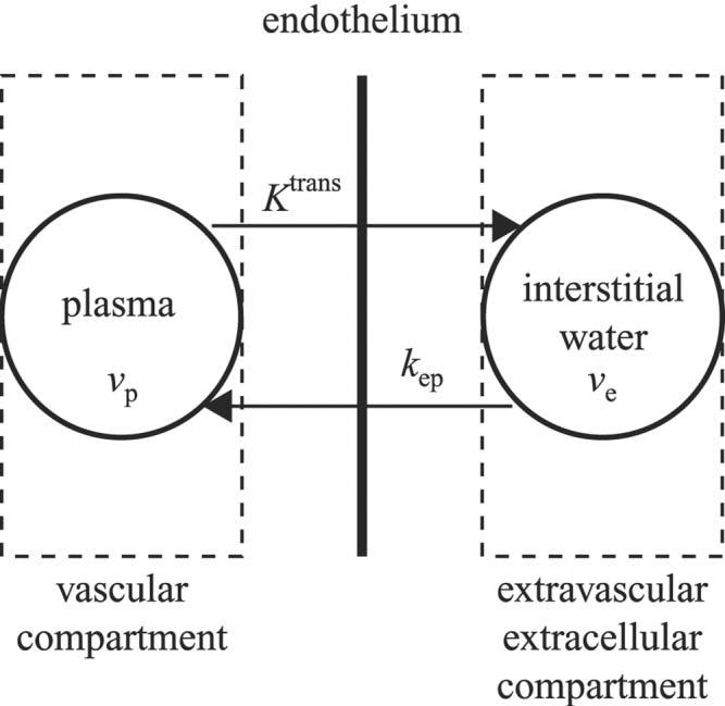
Two-compartment pharmacokinetic model used to model the transport of contrast agent between the vascular compartment and EES. The fractional plasma and EES volumes are denoted by ν_p and ν_e. The transfer constant, K^trans, describes the flux of contrast from the vascular compartment to the EES. The rate constant, k_ep, describes the efflux of contrast from the EES back to the vascular compartment.

FIG. 2.

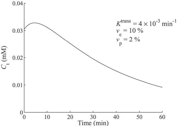
Simulated tissue concentration curve using the Tofts two-compartment model with the following kinetic parameters: K^trans = 4 × 10⁻³ min⁻¹, ν_e = 10%, and ν_p = 2%.

FIG. 3.

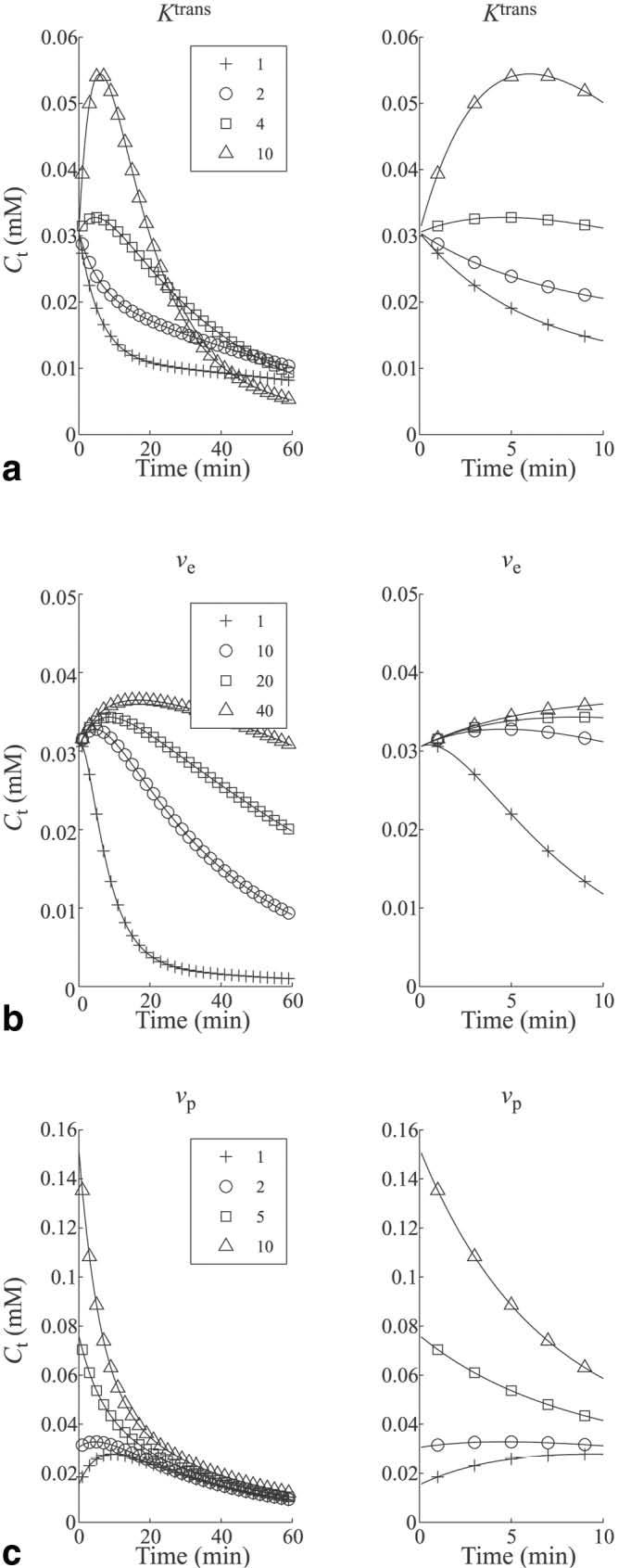
Simulated tissue concentration curves for different kinetic parameter values are shown to illustrate the effect of each individual parameter. Curves are shown for varying values of (a) K^trans (ν_e = 10%, ν_p = 2%), (b) ν_e (K^trans = 4×10⁻³ min⁻¹, v_p = 2%), and (c) ν_p (K^trans = 4×10⁻³ min⁻¹, ν_e = 10%). For each parameter the time course from 0 to 60 min is shown, as well as a magnified version from 0 to 10 min.

From Fig. 3 it can be seen that K^trans influences the initial slope and peak value of C_t. With increasing values of K^trans, contrast is more quickly transferred from the vascular space to the EES, increasing the peak tissue concentration. The v_e parameter primarily effects the washout phase of C_t. As v_e increases, the efflux rate constant k_ep = K^trans/v_e, decreases, and contrast washes out more slowly from the tissue. The v_p parameter determines the initial value of C_t. At t = 0, the integral in Eq. [5] goes to zero and the tissue concentration is equal to the plasma concentration multiplied by the fractional plasma volume. It can be seen from these curves that even for small values of v_p (5%) the shape of C_t is dominated by the shape of the plasma concentration curve, C_p (see Eq. [7]).

MRI Measurements

In Eq. [5], if C_t and C_p are measured, then the other parameters (K^trans, k_ep, and v_p) can be estimated using curve-fitting techniques. To measure C_t and C_p, MR images that are acquired at repeated time points can be used to quantify the changes in contrast agent concentration over time. To accomplish this the following relationship between the contrast agent concentration and the MR spin-lattice relaxation rate (R₁) is used:

$$\Delta R_1=R_1-R_1^0=r_1\left[C\right]$$ [8]

where $R_1^0$ and R₁ are the pre- and postcontrast relaxation rates, respectively; r₁ is the contrast agent relaxivity (13 mM⁻¹ s⁻¹); and [C] is the contrast agent concentration. Eq. [5] can then be rewritten in terms of relaxation rates:

$$\Delta R_{1,\mathrm{t}}=K^{\mathrm{trans}}{\int }_0^t\Delta R_{1,\mathrm{p}}\left(\tau \right)e^{-k_{\mathrm{ep}}(t-\tau )}d\tau +v_{\mathrm{p}}\Delta R_{1,\mathrm{p}}$$ [9]

It is assumed that the contrast agent relaxivity, r₁, is the same in the plasma compartment and EES. Cao and colleagues (17) observed that the relaxivity of Gadomer did not depend on macromolecular content in phantom experiments. This is consistent with the work of Donahue et al. (18), who showed that the relaxivities of Gd-DTPA at 8.5T were the same in saline, plasma, and cartilage (representing interstitium or EES). Work by Stanisz and Henkelman (19), however, showed that the r₁ relaxivity of Gd-DTPA increased with macromolecular concentration at 1.5T. For the present work the relaxivities of Gadomer in the plasma space and EES were assumed to be the same, but it should be noted that the relationship between relaxivity and macromolecular content is a matter of ongoing investigation.

A multislice variant of the Look-Locker sequence, termed T₁ mapping with partial inversion recovery (TAPIR), was used to measure pre- and postcontrast relaxation rates. During a TAPIR acquisition, the signal is acquired repeatedly during T₁ recovery, which results in an apparent relaxation time, T₁*, that is smaller than the true T₁ (20,21). The relationship between the two is a function of the flip angle (α) and the repetition time (TR) and is given by:

$$\frac{1}{{T_1}^{\ast }}=\frac{1}{T_1}-\frac{\ln \left(\cos \left(\alpha \right)\right)}{\mathit{TR}}$$ [10]

Note that the second term in Eq. [10] does not depend on T₁. The change in the true relaxation rate is therefore equal to the change in the apparent relaxation rate:

$$\Delta R_1=\Delta {R_1}^{\ast }$$ [11]

To increase the efficiency of the acquisition, an echo-planar readout was used to acquire four echoes for each TR. A total of 16 slices were acquired, and measurements were made before contrast administration and at regular intervals for approximately 1 hr postcontrast. For each measurement 16 points along the recovery curve were measured for each of the 16 slices in approximately 2 min.

Parameter Estimation Using Linear and Nonlinear Methods

Once the values of ΔR₁ are obtained, Eq. [9] can be used to estimate the parameters K^trans, v_e (= K^trans/k_ep), and v_p. One approach that is often used is to formulate a least-squares optimization problem and use iterative techniques to achieve an optimal solution. Recently methods have been developed to linearize Eq. [5] (22). Murase (22) compared the performance of linear and nonlinear methods in solving the Tofts two-compartment model equation. In that work the values used for the plasma agent concentration (arterial input function (AIF)) and physiological parameters (K^trans, v_e, and v_p) were taken from studies that evaluated the dynamics of an extravascular agent (Gd-DTPA) in tumors. In the case of an intravascular agent, the plasma concentration time-course will differ from that of an extravascular agent. Furthermore, the transfer constant, K^trans, which represents permeability, will be much lower in the case of an intravascular agent, which will likely make it difficult to measure accurately in the presence of noise. Because an intravascular agent distributes only nominally in the extravascular space, measurements of v_e may also be confounded. Therefore, to evaluate the performance of the Tofts two-compartment model in the case of an intravascular tracer, it is important to understand the range of errors one may expect to be associated with parameter estimation.

In our study the performance of the linear (LLSQ) and nonlinear least-squares (NLSQ) methods were evaluated in the case of an intravascular contrast agent and a range of physiologic parameters. The simulations utilized the pharmacokinetics of Gadomer described by Misselwitz et al. (15). Based on Ref. 15, the plasma concentration is assumed to be a bioexponential function defined by Eq. [7]. Rewriting Eq. [5] utilizing Eq. [7] gives (23):

$$C_{\mathrm{t}}=K^{\mathrm{trans}}D\sum _{i=1}^2\left[\frac{a_i}{m_i-k_{\mathrm{ep}}}(e^{-k_{\mathrm{ep}}t}-{\mathrm{e}}^{-m_{i}t})\right]+v_{\mathrm{p}}D\sum _{i=1}^2{a}_i{e}^{-m_{i}t}$$ [12]

or, in terms relaxation rates:

$$\Delta R_{1,\mathrm{t}}=r_1{K}^{\mathrm{trans}}D\sum _{i=1}^2\left[\frac{a_i}{m_i-k_{\mathrm{ep}}}(e^{-k_{\mathrm{ep}}t}-e^{-m_{i}t})\right]+r_1{v}_{\mathrm{p}}D\sum _{i=1}^2{a}_i{e}^{-m_{i}t}$$ [13]

The initial dose of contrast D was set to 0.05 mmol/kg. The plasma concentration time-course was biphasic, with a rapid distribution clearance followed by a slower elimination phase. Monte Carlo simulations were run to analyze the effects of noise on the accuracy of the calculations for the Tofts parameters. To propagate noise from simulated MRI acquisitions to the Tofts model calculations, the following procedure was used:

1. The two-compartment model was used to generate tissue concentration curves using a set of values for K^trans, v_e, and v_p, and a fixed set of plasma parameters (Eq. [12]).

2. Using a simulation model of the TAPIR pulse sequence, a set of T₁* recovery curves were generated that reflected the changing concentrations of contrast in the plasma and tissue compartments.

3. Random, normally distributed noise was added separately to the real and imaginary components of the signal intensity curves.

4. The T₁* values of the noisy signal intensity curves were estimated using nonlinear curve-fitting techniques.

5. The T₁* estimates were converted to the change in relaxation rates (i.e., postcontrast minus precontrast).

6. For the NLSQ method, Eq. [13] was solved using nonlinear optimization techniques.

7. For the LLSQ method, Eq. [13] was solved using linear optimization techniques (see Ref. 22).

The simulations were run for a range of SNR values and kinetic parameters. For each combination, 1000 simulations were run to calculate the mean and standard deviation (SD) for each kinetic parameter. The percent root mean square error (RMSE %) for each parameter was calculated by:

$$\mathit{RMSE}=\sqrt{\sum _{j=1}^N{(({\tilde{P}}_j-P)∕P)}^2∕(N-1)}\times 100$$ [14]

where P̃_j and P are the estimated and true values of the parameter, respectively, and N is the number of simulation runs (22).

The simulations were performed using Matlab (The MathWorks Inc., Natick, MA, USA). Random noise was generated using the randn function. For a desired SNR and equilibrium magnetization (M₀), the noise (σ]) was calculated as σ] =M_o/SNR. Noise was added separately to the real and imaginary components of the signal S to form the noisy signal S_n:

$$S_{\mathrm{n}}=S+\sigma (\mathrm{randn}+j{}^{\ast }\mathrm{randn})$$ [15]

where j =−1.

The data were phase-corrected by subtracting the phase of the most fully relaxed image from the phase of all the images and taking the real part. Computationally, this was accomplished by multiplying each image by e^−jθ, where θ is the phase angle of the most fully relaxed image. The curve-fitting for the T₁* recovery maps was accomplished by fitting the noisy data to a three-parameter equation (24):

$$S_{\mathrm{n}}=A-{\mathit{Be}}^{-\mathit{TI}∕{T_1}^{\ast }}$$ [16]

where A and B are free parameters, TI is the inversion time, and T₁* is the apparent recovery time. In Matlab, the fminsearch function was used, which uses an unconstrained nonlinear optimization technique known as the Nelder-Mead simplex method (25-27).

The Matlab lsqcurvefit function was used to calculate a NLSQ solution to the Tofts equation. This function uses a trust region method that approximates the function to be minimized by a simpler function over a restricted neighborhood, called the trust region (28,29). The preconditioned conjugate gradient method (30) is used to define the 2D subspace trust region at each iteration. Bounds are placed on each parameter to restrict the values of the parameters such that K^trans ∊ [0,∞), v_e ∊ [0,1], and v_p ∊ [0,1].

For the LLSQ method, Eq. [13] was first formulated as a linear equation (22) and then solved using the lsqnonneg function, which implements a linear optimization simplex algorithm (31) and constrains the results to be positive.

Animal Experiments

Experiments were conducted in rabbits to observe the signal intensity kinetics of an intravascular contrast agent in skeletal muscle and determine the feasibility of using the Tofts model to extract K^trans, v_e, and v_p. The animal protocol was approved by the Institutional Animal Care and Use Committee, and was conducted in accordance with National Institutes of Health guidelines. New Zealand White rabbits (N = 5) were intubated and anesthetized with isoflurane and placed supine in the bore of a 1.5 T clinical MRI scanner (General Electric Medical Systems, Waukesha, WI, USA). The animal's legs were elevated and fixed in a custom-made apparatus, and 3-inch receive-only surface coils were placed on the lateral side of each calf. A venous catheter was placed in the ear for administration of fluids and contrast. An arterial catheter was placed in the ear to monitor blood gases. A warm air blower was used to maintain the animal's body temperature.

Initial scout images of the lower limb were used to choose a set of 16 contiguous transverse slices for the contrast experiment. A set of precontrast T₁* maps were acquired using the TAPIR pulse sequence. Gadomer was injected intravenously at a dose of 0.05 mmol/kg, followed by an injection of 10 ml of saline. Sets of T₁* maps were acquired every 2–3 min for 1 hr. For each acquisition, data for 16 points along the inversion recovery curve were collected for all 16 slices with an image resolution of 1.25 mm × 1.25 mm × 4 mm. During reconstruction the images were interpolated by a factor of 2 in-plane. Other imaging parameters were TR/TE/flip = 11.5 ms/2.6 ms/20°.

Data Processing

The complex data were phase-corrected and T₁* maps were generated. For each pixel, ΔR₁ was calculated and the data were fit to Eq. [13] (or its linear form) to calculate K^trans, v_e, and v_p. The signal was measured in the great saphenous artery and fit to a biexponential (see Eq. [7]). The hematocrit was measured from arterial blood samples and was used to convert the blood Gadomer concentration to plasma Gadomer concentration.

Regions of interest (ROIs) were drawn in the TA and SOL muscles of both limbs on spin-echo scout images for four consecutive mid-calf slices, which contained the majority of the SOL muscle. The average ROI volumes were 1835 ± 163 mm³ for the TA and 512 ± 52 mm³ for the SOL. The regions were copied to parametric maps of the Tofts parameters, and mean values were computed for each region. The percent coefficient of variation (CV) within each animal was computed by dividing the SD by the mean value and multiplying by 100 for the eight measurements (four slices times two limbs). The CVs were then averaged across the animals to represent the average intra-animal variability. To compare across animals, the measurements for each muscle were averaged over the four slices, to yield 10 measurements (5 animals × 2 limbs) for each parameter.

Statistical significance was tested using the Wilcoxon rank sum test, and significance was defined as P ≤ 0.05.

RESULTS

Simulation Results

The RMSEs in the Tofts parameters for SNR values of 20–100 are shown in Table 1. The RMSE values were comparable for the NLSQ and LLSQ methods for SNR values above 20, which is consistent with the results of Murase (22). The RMSE values were higher than those obtained with an extravascular agent, due to the lower distribution volume of the intravascular agent.

Table 1.

Root Mean Square Error (RMSE) in Percent (%) for Tofts Parameters for Signal-To-Noise (SNR) Values from 20 to 100^*

SNR	LLSQ			NLSQ
	Ktrans	νe	νp	Ktrans	νe	νp
20	33	77	48	880	91	48
40	15	31	31	15	33	26
60	10	21	21	10	22	17
80	8	16	15	7	17	13
100	6	13	11	6	13	10

^*Values are shown for linear least squares (LLSQ) and nonlinear least squares (NLSQ) methods.

The mean values for each parameter vs. SNR are shown in Fig. 4. Triangles represent values determined by the LLSQ method, and circles represent values determined by the NLSQ method. The error bars are the SD for each set of 1000 runs. For K^trans, the mean and SD are comparable for the LLSQ and NLSQ methods for SNR values above 20, although the LLSQ method seems to slightly underestimate K^trans. For SNR = 20, the mean values are similar, but the SD of the NLSQ method is an order of magnitude larger than the SD of the LLSQ method. The mean and SD values for the two methods are similar for v_e for every SNR value. For v_p, the mean and SD values are similar, but the LLSQ method seems to slightly undestimate the true value, as it did for K^trans. For both methods and all parameters, the SD of the estimates decreased with increasing SNR, as expected.

FIG. 4.

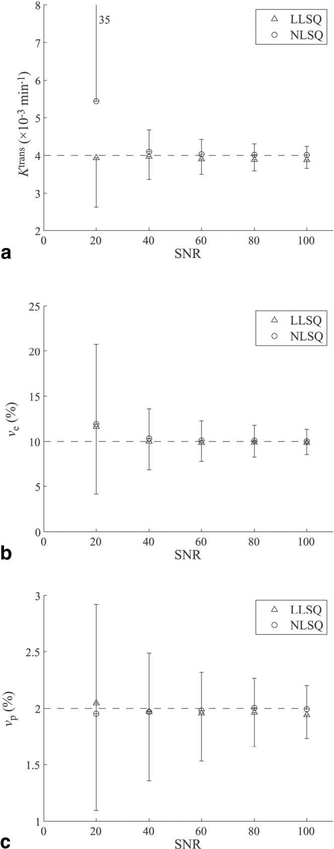
Mean values and SDs for kinetic parameters from Monte Carlo simulations for (a) K^trans, (b) ν_e, and (c) ν_p vs. SNR. As expected, the SD decreases for each parameter with increasing SNR. Values are shown for both the LLSQ method (triangles) and NLSQ method (circles).

The variation of RMSE with different parameter values was also investigated, as shown in Fig. 5. These graphs illustrate the influence that each parameter value has on the parameter estimation error of the model. For each graph the value for two parameters is fixed while the third is varied, and the RMSE is calculated as described above. Each point represents the RMSE for a 1000 Monte Carlo runs at an SNR level of 60. The trends are similar between the LLSQ and NLSQ methods.

FIG. 5.

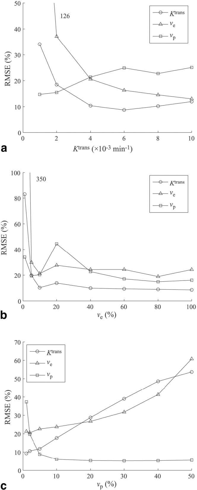
Effect of varying (a) K^trans, (b) ν_e, and (c) ν_p on RMSE for each parameter. Results are shown for the LLSQ method with SNR = 60.

The K^trans RMSE reflects the accuracy in estimating the initial slope of the concentration curve (see Fig. 3). As K^trans increases from 1 to 6 × 10⁻³ min⁻¹, the initial slope increases and the RMSE in K^trans decreases. As K^trans increases from 6 to 10 × 10⁻³ min⁻¹, the slope continues to increase and the measurement becomes hindered by the limited number of data points on the upslope of the curve, resulting in a slight increase of the RMSE. The parameter v_e is related to the later washout portion of the tissue concentration curve. As K^trans increases, the washout slope increases and the accuracy increases. The sampling frequency is sufficient to measure the washout slope throughout the range of K^trans values. The v_p parameter determines the initial value of the tissue concentration curve. For small values of K^trans, the initial data values reflect the plasma volume, but as K^trans increases, the contrast more quickly transfers out of the vascular compartment into the EES, and it becomes more difficult to accurately measure v_p, as demonstrated in Fig. 3. The v_p RMSE increases with increasing values of K^trans until K^trans = 6 × 10⁻³ min⁻¹, where it plateaus.

The effect of v_e is shown in Fig. 5b. For values of v_e below 5%, the RMSE in each of the parameters is fairly high. For low values of v_e, the tissue concentration curve decreases from its initial value of v_pC_p, so the overall SNR is low. As v_e increases, C_t gains an initial positive slope and an increase in SNR. The RMSE of all three parameters stabilizes for v_e > 5%. It is not clear why the v_p RMSE increases at v_e = 20%. A similar peak was not observed for the NLSQ method.

Figure 5c shows the effect of increasing v_p. Larger values of v_p will cause the C_t curve to be dominated by the plasma concentration, C_p, obscuring the effects of K^trans and v_e, increasing the RMSE of these two parameters. The v_p RMSE is higher for low values due to its low SNR, and remains stable after v_p > 5%.

The effect of sampling interval on the RMSE is shown in Table 2. Simulations were run for a sampling interval of 10 min and compared with simulations with a sampling interval of 2 min. The results are for SNR = 60, K^trans = 4 × 10⁻³ min⁻¹, v_e = 10%, and v_p = 2%. The RMSE for all parameters increased with a less frequent sampling interval for both the LLSQ and NLSQ methods.

Table 2.

Effect of Sampling Interval on Parameter RMSE (%)^*

Sampling interval (min.)	LLSQ			NLSQ
	Ktrans	νe	νp	Ktrans	νe	νp
2	10	21	21	10	22	17
10	29	28	30	34	31	24

^*Calculations were done for SNR = 60 and K^trans = 4 × 10⁻³ min⁻¹, ν_e = 10%, and ν_p = 2%.

In Vivo Results

Example precontrast inversion recovery curves for the TA and SOL muscles are shown in Fig. 6. These data were taken from single pixels in each muscle. In the longest-TI image (TI = 2845 ms), the measured SNR (mean signal intensity divided by the SD of the background) in the region of the selected pixels is approximately 140. The solid lines represent fits of the data to Eq. [16]. From the inversion recovery data, ΔR₁ curves were generated, as shown in Fig. 7. Data are shown for pixels within the TA and SOL muscles. The solid lines represent fits of the data to the two-compartment model (Eq. [13]).

FIG. 6.

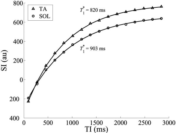
Precontrast inversion recovery curves of pixels in the TA (triangles) and SOL (circles) muscles. The solid lines represent exponential fits to the data, and T₁* is the apparent longitudinal relaxation time.

FIG. 7.

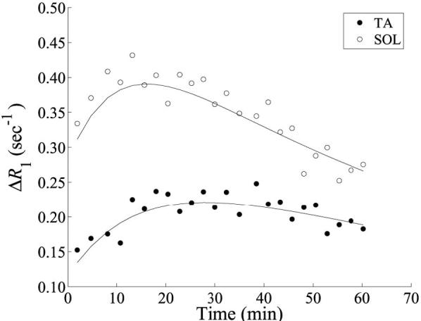
Tissue ΔR₁ curves for the TA and SOL muscles. Circles and dots represent data from single pixels within the TA and SOL regions, respectively. Solid lines are fits of the data to the two-compartment model. For the TA muscle pixel the fit parameters were K^trans = 2.5×10⁻³ min⁻¹, ν_e = 6.4%, and ν_p = 2.0%. For the SOL muscle pixel the fit parameters were K^trans = 4.8×10⁻³ min⁻¹, ν_e = 7.5%, and ν_p = 4.8%.

For each imaging slice, parametric maps were constructed for each kinetic parameter, as shown in Fig. 8. ROIs in the TA and SOL muscles were initially drawn on spin-echo images and then copied over to the parametric maps. Mean values were calculated for each ROI, and the percent CV was calculated for each animal. The average percent CVs for each parameter and muscle are listed in Table 3. The overall mean value for each parameter and muscle group are listed in Table 4. The mean values for K^trans and v_p were significantly higher for the SOL muscle than for the TA muscle. The difference in v_e for the two muscles was not found to be statistically different for this sample.

FIG. 8.

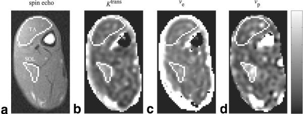
a: Spin-echo image with ROIs drawn for the TA and SOL muscles. Kinetic parameter maps for (b) K^trans,(c) ν_e, and (d) ν_p. The range for the scale bar for each parameter are K^trans: 0–6 × 10⁻³ min⁻¹; ν_e: 0–6%; ν_p: 0–6%.

Table 3.

Average Coeffecient of Variation (%) for Each Parameter for Tibialis Anterior (ANT) and Soleus (SOL) Muscles in Rabbit Hind Limb^*

	ANT	SOL
Ktrans	10	11
νe	14	6
νp	10	8

^*The numbers represent the average variation within each animal, measured over four consecutive slices in both left and right hind limbs (total of eight measurements).

Table 4.

Kinetic Parameter Values for Tibialis Anterior (ANT) and Soleus (SOL) Muscles in Rabbit Hind Limb^*

	ANT	SOL	P-value
Ktrans (× 10−3 min−1)	2.0 ± 0.5	3.2 ± 0.9	<0.01
νe (%)	8.5 ± 1.6	8.7 ± 2.2	N.S.
νp (%)	2.1 ± 0.7	3.4 ± 0.8	<0.01

^*Values are shown as mean ± SD for N = 10 (5 animals × 2 hind limbs). Values for K^trans and v_p are significantly higher in SOL muscle compared with ANT muscle.

DISCUSSION

The two-compartment Tofts model has been most commonly used to study high-permeability, flow-limited tissue with the use of a low molecular weight agent, such as Gd-DTPA. A few groups have used intravascular agents to study tumor vasculature, which is highly permeable compared to vasculature in skeletal muscle. In our study the Tofts model was simulated under conditions that represent the use of an intravascular tracer in skeletal muscle. The effects of image SNR on the accuracy of parameter estimation was examined, as was the influence of the magnitude of each parameter. Experiments were conducted in vivo to assess the feasibility of estimating kinetic parameters in skeletal muscle using the intravascular agent Gadomer.

Noise propagation in the two-compartment model was studied by adding Gaussian noise to simulated images and calculating the resulting RMSE on the parameters. In order to achieve a higher effective SNR, most analyses will average n pixel values within an ROI, giving a $\sqrt{n}$ improvement in SNR. For nominal values of K^trans (4×10⁻³ min⁻¹), v_e (10%) and v_p (2%), the simulations showed that for an SNR value of 20, the RMSE errors may be unacceptably high for both methods, but then there is almost a linear decrease in RMSE with increasing SNR for values from 40 to 100. Similar results were obtained with nonlinear and linear fit methods, although there was a slight underestimation of K^trans and v_p with the linear method. These small residual errors may be an acceptable trade-off, however, for the increased computational efficiency of the linear method. As observed by Murase (22), the linear method is faster than the nonlinear method by a factor of 6.

The measured signal in the tissue concentration curve (C_t) is related directly to the change in relaxation rate caused by the influx of contrast agent. The magnitude of this change is in turn related to the distribution volume of the agent. For low-molecular-weight agents the distribution volume is the vascular space and EES space, or 10–20% of the tissue volume. For high-molecular-weight intravascular agents, the distribution volume is primarily the plasma space (2–5%) and to some degree the EES, which is influenced by K^trans. In general, increased values of K^trans and v_e will cause a greater amount of contrast to be transferred from the plasma space to the EES, increasing the initial slope and peak of the tissue concentration curve. This increased signal results in an overall decrease in RMSE. The effect of sampling frequency may confound this trend, however, if the temporal resolution is not sufficient to capture the initial slope of C_t, which makes it important to have an estimation of the contrast kinetics when designing the imaging experiment. From a signal-processing perspective, one could analyze the frequency content of the initial portion of the anticipated C_t curve and use this to choose an appropriate sampling period. For a typical curve, as shown in Fig. 2, at a minimum one should have at least three sample points before the peak of the curve.

For the in vivo experiments, the values of K^trans and v_p were found to be significantly higher in the SOL muscle compared to the TA muscle. This is consistent with the physiological differences between the two muscles. The SOL muscle is comprised primarily of “slow-twitch” type I fibers and is more vascularized than the TA muscle, which consists mostly of “fast-twitch” type II fibers (32). The SOL muscle therefore has a larger capillary surface area. This increases both K^trans, which represents the permeability surface area product, and v_p, the fractional plasma volume. Similar results were found by Vincensini et al. (33), who used a two-compartment model and Gd-DTPA to investigate capillary permeability in rabbit skeletal muscle. They found that the permeability of the slow-twitch semimembranosus proprius muscle was about twice that of the fast-twitch semimembranosus muscle (0.25 min⁻¹ vs. 0.13 min⁻¹). They also found differences in the extracellular volume fraction (v_e) between the two types of muscles (0.189 vs. 0.095 for the semimembranosus proprius and semimembranosus, respectively)—a finding that was not seen in the current study. This may be due to inherent physiological differences between the muscles examined in this study and the muscles examined by Vincensini's group.

It is important to note that the permeability represented by K^trans in this study is the permeability of the vasculature to Gadomer—not water, as described by Schwarzbauer et al. (10). Because Gadomer is ∼30 times larger than Gd-DTPA, the permeability is much lower. For example, compared to values found by Vincensini et al. (33), the K^trans values in this study are two orders of magnitude lower. There are two advantages to using an intravascular agent instead of an extravascular agent for detecting permeability changes. The first is that with a macromolecular agent, flux is more likely to be permeability limited, so that K^trans approximately equals the permeability surface area product. In the case of a low-molecular-weight agent, the flux is more likely to be flow-limited, and K^trans will reflect the bulk blood flow rate (7). The second advantage is that the lower flux rate increases the overall time course of the contrast kinetics, enabling measurements with greater resolution and/or coverage. In the case of Gd-DTPA, it is difficult to sufficiently sample the tissue concentration curve for more than one slice, and often only the relative signal intensity is measured rather than the actual relaxation rate. With an intravascular agent, it is possible to make accurate relaxation rate maps for multiple slices with sufficient sampling frequency, as demonstrated in this study.

One potential limitation of the current study is that the plasma signal was measured directly from the MRI images from the great saphenous artery. At the level of the most superior slice, this vessel had a diameter of <2 mm, containing either a 2 × 2 or 3 × 3 set of pixels (in images that had been interpolated to 0.63 mm in-plane resolution). With this limited resolution, vessel motion and partial volume effects could impact the measurements. Ideally, the plasma signal measurement would come from a large vessel, such as the descending aorta, so that many pixels could be averaged to increase the SNR of the measurement. However, such measurements would require a separate imaging slice to obtain this input function with additional estimates of the delay in delivery of the contrast agent.

The influence of water exchange may play an important role in parameter estimation (17,34,35). There are three sites of exchange to consider: the red blood cells, the vascular endothelial wall, and the parenchymal cells in the extravascular space. The Tofts model presented here assumes that proton exchange at each of these sites is in the limit of fast exchange, i.e., the proton exchange rate across these boundaries is much faster than the difference in relaxation rates between the compartments. In the fast exchange limit, the water from multiple compartments relaxes according to a single relaxation rate constant that is a weighted sum of the relaxation rates of the individual compartments. In cases in which the fast exchange limit does not apply, then the different compartments each relax according to different time constants. In the case of red blood cells, the exchange rate is approximately 100 s⁻¹ (35). For a dose of Gadomer of 0.05 mmol/kg, the peak plasma concentration will be approximately 1.2 mM, and the peak R₁ will be 16 s⁻¹ (the peak ΔR₁ will be 15 s⁻¹, assuming a precontrast plasma R₁ of approximately 1 s). Since this is an order of magnitude less than the water exchange rate, the assumption that the water is in fast exchange across the red blood cell boundary is valid. Thus, the blood pool can be considered as a single compartment. For cells outside of the vascular space, the transcytolemmal water exchange rates may be much lower than those for red blood cells. Landis et al. (34) measured this exchange rate in rat thigh muscle to be approximately 0.8 s⁻¹ in vivo. Similarly, transendothelial exchange rates have been estimated to be 1–6 s⁻¹ in myocardium (18,35). Several approaches have been proposed to account for the effect of water exchange on the relaxation kinetics (34,36,37), although a consensus has yet to emerge on how to best account for these effects and how to balance the need for additional model parameters and the limited precision of the measurements. In the worstcase scenario, the consequence of assuming fast exchange where it does not exist is the underestimation of v_p and the overestimation of K^trans (17,38).

In conclusion, the current study demonstrates the feasibility of measuring tissue kinetic parameters in skeletal muscle using the intravascular agent Gadomer and the Tofts two-compartment model. In particular, this method is capable of measuring vascular differences between the fast-twitch TA and slow-twitch SOL muscles in the rabbit. The approach described here may be useful for assessing changes in vascular volume or permeability in settings of ischemia or proangiogenic treatment.

REFERENCES

- 1.Tofts PS, Kermode AG. Measurement of the blood–brain barrier permeability and leakage space using dynamic MR imaging. 1. Fundamental concepts. Magn Reson Med. 1991;17:357–367. doi: 10.1002/mrm.1910170208. [DOI] [PubMed] [Google Scholar]
- 2.Ewing JR, Knight RA, Nagaraja TN, Yee JS, Nagesh V, Whitton PA, Li L, Fenstermacher JD. Patlak plots of Gd-DTPA MRI data yield blood–brain transfer constants concordant with those of 14C-sucrose in areas of blood–brain opening. Magn Reson Med. 2003;50:283–292. doi: 10.1002/mrm.10524. [DOI] [PubMed] [Google Scholar]
- 3.Keijer JT, Bax JJ, van Rossum AC, Visser FC, Visser CA. Myocardial perfusion imaging: clinical experience and recent progress in radionuclide scintigraphy and magnetic resonance imaging. Int J Card Imaging. 1997;13:415–431. doi: 10.1023/a:1005737725964. [DOI] [PubMed] [Google Scholar]
- 4.Gillies RJ, Bhujwalla ZM, Evelhoch J, Garwood M, Neeman M, Robinson SP, Sotak CH, Van Der SB. Applications of magnetic resonance in model systems: tumor biology and physiology. Neoplasia. 2000;2:139–151. doi: 10.1038/sj.neo.7900076. [DOI] [PMC free article] [PubMed] [Google Scholar]
- 5.Brasch R, Pham C, Shames D, Roberts T, vanDijke K, vanBruggen N, Mann J. Ostrowitzki S, Melnyk O. Assessing tumor angiogenesis using macromolecular MR imaging contrast media. J Magn Reson Imaging. 1997;7:68–74. doi: 10.1002/jmri.1880070110. [DOI] [PubMed] [Google Scholar]
- 6.Bhujwalla ZM, Artemov D, Natarajan K, Ackerstaff E, Solaiyappan M. Vascular differences detected by MRI for metastatic versus nonmeta-static breast and prostate cancer xenografts. Neoplasia. 2001;3:143–153. doi: 10.1038/sj.neo.7900129. [DOI] [PMC free article] [PubMed] [Google Scholar]
- 7.Tofts PS, Brix G, Buckley DL, Evelhoch JL, Henderson E, Knopp MV, Larsson HB, Lee TY, Mayr NA, Parker GJ, Port RE, Taylor J, Weisskoff RM. Estimating kinetic parameters from dynamic contrast-enhanced T-weighted MRI of a diffusable tracer: standardized quantities and symbols. J Magn Reson Imaging. 1999;10:223–232. doi: 10.1002/(sici)1522-2586(199909)10:3<223::aid-jmri2>3.0.co;2-s. [DOI] [PubMed] [Google Scholar]
- 8.Su MY, Muhler A, Lao X, Nalcioglu O. Tumor characterization with dynamic contrast-enhanced MRI using MR contrast agents of various molecular weights. Magn Reson Med. 1998;39:259–269. doi: 10.1002/mrm.1910390213. [DOI] [PubMed] [Google Scholar]
- 9.Henderson E, Sykes J, Drost D, Weinmann HJ, Rutt BK, Lee TY. Simultaneous MRI measurement of blood flow, blood volume, and capillary permeability in mammary tumors using two different contrast agents. J Magn Reson Imaging. 2000;12:991–1003. doi: 10.1002/1522-2586(200012)12:6<991::aid-jmri26>3.0.co;2-1. [DOI] [PubMed] [Google Scholar]
- 10.Schwarzbauer C, Morrissey SP, Deichmann R, Hillenbrand C, Syha J, Adolf H, Noth U, Haase A. Quantitative magnetic resonance imaging of capillary water permeability and regional blood volume with an intravascular MR contrast agent. Magn Reson Med. 1997;37:769–777. doi: 10.1002/mrm.1910370521. [DOI] [PubMed] [Google Scholar]
- 11.Wilke N, Kroll K, Merkle H, Wang Y, Ishibashi Y, Xu Y, Zhang J, Jerosch-Herold M, Muhler A, Stillman AE. Regional myocardial blood volume and flow: first-pass MR imaging with polylysine-Gd-DTPA. J Magn Reson Imaging. 1995;5:227–237. doi: 10.1002/jmri.1880050219. [DOI] [PMC free article] [PubMed] [Google Scholar]
- 12.Demsar F, Roberts TP, Schwickert HC, Shames DM, van Dijke CF, Mann JS, Saeed M, Brasch RC. A MRI spatial mapping technique for microvascular permeability and tissue blood volume based on macromolecular contrast agent distribution. Magn Reson Med. 1997;37:236–242. doi: 10.1002/mrm.1910370216. [DOI] [PubMed] [Google Scholar]
- 13.Roberts HC, Saeed M, Roberts TP, Muhler A, Shames DM, Mann JS, Stiskal M, Demsar F, Brasch RC. Comparison of albumin-(Gd-DTPA)30 and Gd-DTPA-24-cascade-polymer for measurements of normal and abnormal microvascular permeability. J Magn Reson Imaging. 1997;7:331–338. doi: 10.1002/jmri.1880070213. [DOI] [PubMed] [Google Scholar]
- 14.Bhujwalla ZM, Artemov D, Natarajan K, Solaiyappan M, Kollars P, Kristjansen PE. Reduction of vascular and permeable regions in solid tumors detected by macromolecular contrast magnetic resonance imaging after treatment with antiangiogenic agent TNP-470. Clin Cancer Res. 2003;9:355–362. [PubMed] [Google Scholar]
- 15.Misselwitz B, Schmitt-Willich H, Ebert W, Frenzel T, Weinmann HJ. Pharmacokinetics of Gadomer-17, a new dendritic magnetic resonance contrast agent. MAGMA. 2001;12:128–134. doi: 10.1007/BF02668094. [DOI] [PubMed] [Google Scholar]
- 16.Tofts PS. Modeling tracer kinetics in dynamic Gd-DTPA MR imaging. J Magn Reson Imaging. 1997;7:91–101. doi: 10.1002/jmri.1880070113. [DOI] [PubMed] [Google Scholar]
- 17.Cao Y, Brown SL, Knight RA, Fenstermacher JD, Ewing JR. Effect of intravascular-to-extravascular water exchange on the determination of blood-to-tissue transfer constant by magnetic resonance imaging. Magn Reson Med. 2005;53:282–293. doi: 10.1002/mrm.20340. [DOI] [PubMed] [Google Scholar]
- 18.Donahue KM, Burstein D, Manning WJ, Gray ML. Studies of Gd-DTPA relaxivity and proton exchange rates in tissue. Magn Reson Med. 1994;32:66–76. doi: 10.1002/mrm.1910320110. [DOI] [PubMed] [Google Scholar]
- 19.Stanisz GJ, Henkelman RM. Gd-DTPA relaxivity depends on macromolecular content. Magn Reson Med. 2000;44:665–667. doi: 10.1002/1522-2594(200011)44:5<665::aid-mrm1>3.0.co;2-m. [DOI] [PubMed] [Google Scholar]
- 20.Steinhoff S, Zaitsev M, Zilles K, Shah NJ. Fast T mapping with volume coverage. Magn Reson Med. 2001;46:131–140. doi: 10.1002/mrm.1168. [DOI] [PubMed] [Google Scholar]
- 21.Zaitsev M, Steinhoff S, Shah NJ. Error reduction and parameter optimization of the TAPIR method for fast T1 mapping. Magn Reson Med. 2003;49:1121–1132. doi: 10.1002/mrm.10478. [DOI] [PubMed] [Google Scholar]
- 22.Murase K. Efficient method for calculating kinetic parameters using T1-weighted dynamic contrast-enhanced magnetic resonance imaging. Magn Reson Med. 2004;51:858–862. doi: 10.1002/mrm.20022. [DOI] [PubMed] [Google Scholar]
- 23.Verhoye M, van der Sanden BP, Rijken PF, Peters HP, Van der Kogel AJ, Pee G, Vanhoutte G, Heerschap A, Van der LA. Assessment of the neovascular permeability in glioma xenografts by dynamic T MRI with Gadomer-17. Magn Reson Med. 2002;47:305–313. doi: 10.1002/mrm.10072. [DOI] [PubMed] [Google Scholar]
- 24.Crawley AP, Henkelman RM. A comparison of one-shot and recovery methods in T1 imaging. Magn Reson Med. 1988;7:23–34. doi: 10.1002/mrm.1910070104. [DOI] [PubMed] [Google Scholar]
- 25.Nelder JA, Mead R. A simplex method for function minimization. Comput J. 1965;7:308–313. [Google Scholar]
- 26.Lagarias JC, Reeds JA, Wright MH, Wright PE. Convergence properties of the Nelder-Mead simplex method in low dimensions. Siam J Optimiz. 1998;9:112–147. [Google Scholar]
- 27.Bertsekas DP. Nonlinear programming. 2nd ed. Athena Scientific; 1999. Direct search methods; pp. 162–165. [Google Scholar]
- 28.Coleman TF, Li YY. An interior trust region approach for nonlinear minimization subject to bounds. Siam J Optimiz. 1996;6:418–445. [Google Scholar]
- 29.Bertsekas DP. Nonlinear programming. 2nd ed. Athena Scientific; 1999. Trust region methods; pp. 96–98. [Google Scholar]
- 30.Bertsekas DP. Nonlinear programming. 2nd ed. Athena Scientific; 1999. Preconditioned conjugate gradient method; pp. 138–139. [Google Scholar]
- 31.Lawson CL, Hanson RJ. Solving least squares problems. Prentice-Hall; 1974. p. 161. [Google Scholar]
- 32.Wang LC, Kernell D. Fibre type regionalisation in lower hindlimb muscles of rabbit, rat and mouse: a comparative study. J Anat. 2001;199(Pt 6):631–643. doi: 10.1046/j.1469-7580.2001.19960631.x. [DOI] [PMC free article] [PubMed] [Google Scholar]
- 33.Vincensini D, Dedieu V, Renou JP, Otal P, Joffre F. Measurements of extracellular volume fraction and capillary permeability in tissues using dynamic spin-lattice relaxometry: studies in rabbit muscles. Magn Reson Imaging. 2003;21:85–93. doi: 10.1016/s0730-725x(02)00638-0. [DOI] [PubMed] [Google Scholar]
- 34.Landis CS, Li X, Telang FW, Molina PE, Palyka I, Vetek G, Springer CS., Jr Equilibrium transcytolemmal water-exchange kinetics in skeletal muscle in vivo. Magn Reson Med. 1999;42:467–478. doi: 10.1002/(sici)1522-2594(199909)42:3<467::aid-mrm9>3.0.co;2-0. [DOI] [PubMed] [Google Scholar]
- 35.Donahue KM, Weisskoff RM, Burstein D. Water diffusion and exchange as they influence contrast enhancement. J Magn Reson Imaging. 1997;7:102–110. doi: 10.1002/jmri.1880070114. [DOI] [PubMed] [Google Scholar]
- 36.Bjornerud A, Bjerner T, Johansson LO, Ahlstrom HK. Assessment of myocardial blood volume and water exchange: theoretical considerations and in vivo results. Magn Reson Med. 2003;49:828–837. doi: 10.1002/mrm.10430. [DOI] [PubMed] [Google Scholar]
- 37.Buckley DL. Transcytolemmal water exchange and its affect on the determination of contrast agent concentration in vivo. Magn Reson Med. 2002;47:420–424. doi: 10.1002/mrm.10098. [DOI] [PubMed] [Google Scholar]
- 38.Donahue KM, Weisskoff RM, Chesler DA, Kwong KK, Bogdanov AA, Jr, Mandeville JB, Rosen BR. Improving MR quantification of regional blood volume with intravascular T1 contrast agents: accuracy, precision, and water exchange. Magn Reson Med. 1996;36:858–867. doi: 10.1002/mrm.1910360608. [DOI] [PubMed] [Google Scholar]