Automated classification of lung bronchovascular anatomy in CT using AdaBoost

Abstract

Lung CAD systems require the ability to classify a variety of pulmonary structures as part of the diagnostic process. The purpose of this work was to develop a methodology for fully automated voxel-by-voxel classification of airways, fissures, nodules, and vessels from chest CT images using a single feature set and classification method. Twenty-nine thin section CT scans were obtained from the Lung Image Database Consortium (LIDC). Multiple radiologists labeled voxels corresponding to the following structures: airways (trachea to 6th generation), major and minor lobar fissures, nodules, and vessels (hilum to peripheral), and normal lung parenchyma. The labeled data was used in conjunction with a supervised machine learning approach (AdaBoost) to train a set of ensemble classifiers. Each ensemble classifier was trained to detect voxels part of a specific structure (either airway, fissure, nodule, vessel, or parenchyma). The feature set consisted of voxel attenuation and a small number of features based on the eigenvalues of the Hessian matrix (used to differentiate structures by shape). When each ensemble classifier was composed of 20 weak classifiers, the AUC values for the airway, fissure, nodule, vessel, and parenchyma classifiers were 0.984 ± 0.011, 0.949 ± 0.009, 0.945 ± 0.018, 0.953 ± 0.016, and 0.931± 0.015 respectively. The strong results suggest that this could be an effective input to higher-level anatomical based segmentation models with the potential to improve CAD performance.

1. INTRODUCTION

The clinical motivation for this research is to improve the feasibility and accuracy of computer aided diagnosis (CAD) for pulmonary disease. Lung CAD has the potential to play a critical role in accomplishing a range of quantitative tasks; including, early cancer and disease detection, analysis of disease progression, analysis of pulmonary function and perfusion, and automate identification and tracking of implanted devices (FDA, 2006). A fully automated approach for the robust detection and segmentation of bronchovascular anatomy is an essential, yet challenging, step in building a lung CAD system.

Many effective methods have been developed for specific tasks, such as airway segmentation and quantitative evaluation (Palágyi et al., 2005; Park et al., 1998), fissure identification (Saita et al., 2004; Zhang et al., 2006; Zhou et al., 2004), nodule detection (Armato et al., 2001; Brown et al., 2003; Fiebich et al., 1999), and vessel segmentation (Agam et al., 2005; Krissian et al., 2000; Pizer et al. 2003; Pock et al. 2005). These methods commonly apply a structure specific pre-processing step prior to a final segmentation algorithm. A medialness function has been used prior to higher level algorithms for vessel and airway segmentation (Krissian et al. 2000; Pizer et al. 2003; Pock et al. 2005). Enhancement filters, ridgeness measures, and edge detectors have been applied for fissures during lobar segmentation (Saita et al., 2004; Zhang et al., 2006; Zhou et al., 2004). A vessel enhancement stage has been shown to reduce false positives during nodule detection (Agam et al. 2005). These enhancement stages all utilize attenuation and shape information, yet so far their implementation has always been structure specific.

The aim of this work is to develop a fully automated approach for a voxel-by-voxel classification of multiple structures (airways, fissures, nodules, and vessels) using a single feature set and classification method. Such an approach should be more versatile and practical than developing and implementing multiple methods for each structure. The voxel-by-voxel classification is intended to be a precursor step prior to higher-level anatomical based segmentation models, and an alternative to structure specific enhancement filters (Agam et al., 2005; Frangi et al., 1998; Sato et al., 1997; van Rikxoort and van Ginnekan, 2006; Wiemker et al., 2005).

The underlying hypothesis of this investigation is that lung bronchovascular anatomy can be differentiated on CT by a small but powerful feature set consisting of attenuation and shape descriptors (based on the eigenvalues of the Hessian matrix). An emphasis was placed on a strong a priori knowledge of the feature space and the discriminative ability of the feature set. Pattern recognition techniques were used to avoid heuristically chosen features, thresholds, and parameters. The AdaBoost machine learning algorithm was chosen for its strong theoretical basis and ability to concurrently select and combine relevant features from the feature set during the training of each independent classifier (one per structure). The transparency of the algorithm allows an understanding of the feature selection process and verification that the selected features match the a priori belief on the discriminative ability of the feature set.

A review of the features, AdaBoost, and evaluation dataset is presented in Section 2. A quantitative review of the feature space, feature selection, classifier performance, comparison to standard enhancement filters, and illustration of the application of the method to region-based segmentation is presented in Section 3. The potential and limitations of the approach are discussed in Section 4.

2. METHODS

The paper describes an approach for voxel-by-voxel classification of airways, fissures, nodules, vessels, and normal parenchyma that utilizes a single feature set and classification algorithm. A review of the feature computation is presented followed by a review of the AdaBoost machine learning algorithm, which was used to train one ensemble classifier per structure. A description of the dataset and methods for quantitative evaluation of the classification is also provided.

2.1. Feature set

The feature set was selected to enable detection of structures of various shapes and sizes. The eigenvalues of the Hessian matrix are used for gradient based shape analysis. A multiscale approach is used to improve the detection of various size structures.

2.1.1. Eigenvalue computation

The Hessian matrix is a matrix of second order partial derivatives (Eq. 1) and measures the 2^nd order variations in intensity about a point. The computation has been described in greater detail by other authors (Frangi et al., 1998; Krissian et al., 2000; Sato et al., 1998). The eigenvalues of the Hessian matrix are represented as κ₁, κ₂, κ₃, and are ranked according to their absolute value |κ₁| > |κ₂| > |κ₃|.

$$Hf(x,y,z)=\left[\begin{array}{ccc}{f}_{xx}& f_{yx}& f_{zx}\\ f_{xy}& f_{yy}& f_{zy}\\ f_{xz}& f_{yz}& f_{zz}\end{array}\right]$$ (1)

Multiscale analysis is performed by computing the Hessian matrix (and eigenvalues) at multiple scales. The scale, σ, refers to the amount of smoothing applied to the image (i.e. the standard deviation of the Gaussian smoothing kernel). Since the voxel dimensions of CT images are typically not isotropic, the voxel size along each axis is used when computing the second order partial derivatives of the Hessian matrix (i.e. resulting in units of HU/mm²), and also when determining the size of the Gaussian smoothing kernel.

The scales used in this study {σ = 0.7, 1.0, 1.6, 2.4, 3.5, and 6.0 mm} were chosen to correspond to the size of the structures of interest. The range of scales allows the shape of both larger and smaller objects to be detected and quantified (Florack et al., 1992; Frangi et al., 1998; Krissian et al., 2000; Lindeberg, 1994; Pock, et al., 2005). At lower scales, the shape of larger structures may not be accurately captured due to noise and small inhomogeneities in the structure. At higher scales, the shape of smaller objects may be distorted as neighboring structures are smoothed together. Multiplying the eigenvalues by the scale theoretically normalize the response across scales and provides a means for determining the size of an object based on the scale at which the highest response occurred.

2.1.2. Derived features

The simple feature set consists of voxel attenuation and a small number of features based on the eigenvalues of the Hessian matrix (to differentiate structures by shape). This is similar to features used by previous authors for structure enhancement (Frangi et al., 1998; Wiemker et al., 2005). The gradient based features take advantage of the fact that CT attenuation is a measure of the mean attenuation of tissues occupying each voxel and should have a similar range for a given structure across calibrated CT scanners (Brushberg et al. 2002).

Since the full complexity of shapes cannot be captured by a single feature, multiple features are computed using the eigenvalues (κ₁, κ₂, and κ₃) of the Hessian matrix. The sign and magnitude of each eigenvalue is proportional to the change in attenuation gradient along its corresponding eigenvector. The magnitude of the eigenvalues, $\sqrt{{\kappa }_1^2+{\kappa }_2^2+{\kappa }_3^2}$, is a measure of object contrast compared the local background (i.e. larger eigenvalues will correspond to higher gradients and higher magnitude). Various ratios between the eigenvalues (|κ₂/κ₁|, |κ₃/κ₁|, $\frac{\mid {\kappa }_1\mid -\mid {\kappa }_2\mid }{\mid {\kappa }_1\mid +\mid {\kappa }_2\mid }$, and $\frac{\mid {\kappa }_3\mid }{\sqrt{\mid {\kappa }_1{\kappa }_2\mid }}$) are intended to differentiate structures based on the predicted eigenvalue relationships for different shapes (Figure 1). κ₁ is expected to be relatively larger for all structures than parenchyma. κ₂ is expected to be relatively larger for airways, vessels, and nodules than fissures or parenchyma. κ₃ is expected to be small for all structures except nodules. The eigenvalues and shape features are computed at each scale along with the max and min (based on magnitude) of the feature over all scales.

Figure 1.

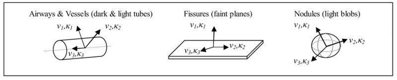
Illustration of bronchovascular structures and predicted eigenvectors/eigenvalue pairs.

Figure 1 illustrates the theoretical basis for the feature set based on the predicted eigenvectors and eigenvalues for each bronchovascular structure.

Airways and vessels are modeled as dark and light tubes respectively. The two largest eigenvalues (κ₁ and κ₂) should correspond to the attenuation change along the eigenvectors in the direction from inside to outside of the airway or vessel (ν₁ and ν₂). The sign of κ₁ and κ₂ is expected to be positive for airways (since airways are darker than airway walls and surrounding tissues) and negative for vessels (since vessels are lighter than parenchyma). The smallest eigenvalue (κ₃) should correspond to the eigenvector (ν₃) in the direction of the trajectory of the airway or vessel.

Fissures are modeled as faint, plate like structures due to their thin surface and partial volume averaging. κ₁ should correspond to the gradient change normal to the fissure plane (along ν₁). The other two eigenvalues (κ₂ and κ₃) should correspond to the eigenvectors (ν₂ and ν₃) in-plane with the fissure and should be closer to zero. Nodules, or faint to bright blob like structures, are expected to have three large negative eigenvalues corresponding to the attenuation change from inside to outside of the nodule in any direction. Non-diseased lung parenchyma lacks structure and would be expected to have three eigenvalues close to zero; however, the eigenvalues of parenchyma near the edge or between structures are likely to show a varied response.

An investigation of the feature space for the reference dataset in this study is presented in Figure 4.

Figure 4.

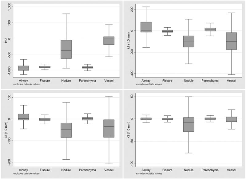
Distribution of attenuation and eigenvalues features (computed at a scale of 1.0 mm) for the bronchovascular structures. The median, upper/lower hinge of the 75^th percentile, and whiskers with upper/lower adjacent values are shown. Outlier values are not shown.

2.2. AdaBoost machine learning

The AdaBoost machine learning algorithm was used to train one ensemble classifier per structure (Freund and Schapire, 1997). AdaBoost is a relatively new algorithm that was selected based on its strong theoretical basis, simplicity to implement, transparency of feature selection, and performance for discriminative tasks (Schapire, 2001; Viola and Jones, 2001). The algorithm concurrently selects and combines relevant features from the feature set during the training of each independent classifier, thus avoiding a separate feature selection process common with other classification methods. The basic premise of the algorithm is that any number of weak classifiers with an error rate less than 50% can be combined to form an ensemble classifier whose error rate approaches that of an optimal classifier.

2.2.1. Weak classifier (feature) selection

As outlined in Figure 2, the AdaBoost algorithm determines the optimal combination of T weak classifiers {h₁(x)…h_T(x)}, chosen from any number of possible weak classifiers, when training the ensemble classifier for each structure. For generalization of results to an unseen dataset, simple weak classifiers that differentiate structures based on a threshold condition of a single feature were employed. A semi-exhaustive search technique was used to train the weak classifiers, where the decision threshold of the weak classifier was tested using values from a random selection of positive samples. The output of each weak classifier is either 1 or 0 for positive and negative classifications respectively, h_t(x) = {1,0}.

Figure 2.

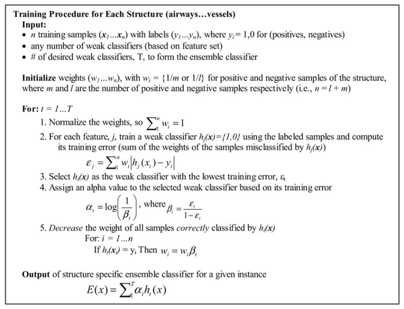
Outline of AdaBoost algorithm adapted from Freund and Schapire, 1997 and Viola and Jones, 2001. The algorithm iteratively selects and combines a small number of features to train each structure specific ensemble classifier.

Weak classifiers are iteratively selected based on their training error for a given set of n training samples (x₁…x_n) with labels (y₁…y_n). Each label is 1 or 0, depending on whether or not the sample is a positive example of the structure the ensemble classifier is being trained to detect. Weights assigned to each training sample {w_i…w_n} are used to determine the training error. The weights are initialized so that the cost of misclassification is the same for each structure. During each iteration, the weak classifier with the lowest training error (sum of the weights of misclassified samples) is selected and the weights of correctly classified samples are decreased. The sample weights allow the algorithm to adaptively select weak classifiers sensitive for samples misclassified during previous iterations (i.e. samples with higher weights, since they cost more to misclassify).

Further analysis of the weak classifier selection and the influence of the number of weak classifiers on ensemble classifier performance is presented Section 3.2 and Section 3.3 respectively.

2.2.2. Voxel classification

As mentioned, one ensemble classifier is trained for each structure. The output of each ensemble classifier is the sum of the alpha values of the weak classifiers whose classification condition has been met. The alpha values are assigned based on the training error of each selected weak classifier and allow the algorithm to optimally combine the set of weak classifiers so that weak classifiers with lower training error have greater impact on the classification decision.

The set of ensemble classifiers can be used independently or for a unique classification of each voxel. When used independently, a binary classification of the structure is formed when the ensemble output (alpha sum) for a given voxel is above a pre-determined classification threshold (ROC point) for that structure. Using the classifiers independently does not ensure a unique labeling of each voxel; since multiple structure classifiers may positively classify the voxel. To assign one unique label, the likelihood of a voxel being part of each structure can be computed using the output of each ensemble classifier. The voxel is then labeled as the structure with the highest likelihood.

2.3. Reference dataset

Twenty-nine publicly available thin section chest CT series were obtained from the Lung Image Database Consortium (LIDC, 2006). There were 28 subjects total, with one subject being scanned on two separate scanners. The images were acquired on 10 scanner models from 4 manufacturers (General Electric, Philips, Siemens, and Toshiba). The peak tube current potentials were 120 kVp (n=20), 130 kVp (n=1), 135 kVp (n=4), and 140 kVp (n=4). The tube current ranged from 40 mA to 486 mA (mean 178 mA). The in-plane voxel size of the 512x512 images ranged from 0.54 to 0.75 mm (mean 0.66 mm). The slice thicknesses were 1.25 mm (n=1), 1.5 mm (n=2), 2.0 mm (n=11), 2.5 mm (n=10), and 3.0 mm (n=5). The reconstruction intervals ranged from 0.75 mm to 3.0 mm (mean 1.94 mm). Intravenous contrast was administered in 10 scans. Reconstruction kernels vary between manufacturers, but in general these cases were reconstructed with standard or slightly enhancing reconstruction kernels. All subjects were scanned at full inspiration.

A reference dataset was compiled from two sources: one for nodules and one for all other structures. The labeled voxels for nodules were derived from radiologist markings in the public LIDC database. Markings indicated as nodules (either < 3 mm or ≥ 3 mm) by at least two of the four radiologists were defined as nodules (Ochs et. al, 2007). For this study, a limited number of points were taken from the center of each nodule in order to avoid possible bias from having more points from larger nodules than from smaller nodules.

The labeled voxels for airways, fissures, non-diseased parenchyma, and vessels was obtained from four additional radiologists (not part of the LIDC reading team), who each read a randomly assigned subset of the 29 cases (7 to 8 cases each). For each case, radiologists were instructed to label a minimum of 75 non-neighboring voxels (at least 1.0 mm apart and preferably distributed equally throughout the lung region) for each of the following eight categories: 1) trachea and main stem bronchus, defined as 0^th and 1^st generation airways, 2) lobar level, 2^nd, to 6^th generation airways, 3) visible portions of the major fissure, 4) visible portions of the minor fissure, 5) lung parenchyma within 2 mm of structures such as the chest wall and vessels, 6) lung parenchyma in the open at least 2 mm from structures, 7) hilum and lobar level arteries and veins, and 8) segmental to peripheral arteries and veins. In total, the radiologists marked over 19 000 points in the 29 cases. Figure 3 shows examples of radiologist labeled voxels.

Figure 3.

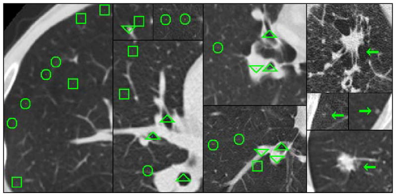
Illustration of radiologist labeled image data. Radiologists marked voxels airways (indicated by triangles), fissures (circles), parenchyma (squares), and vessels (upside-down triangles). Examples of marked nodules from the LIDC database are indicated with arrows.

2.4. Statistical analysis

Each structure specific ensemble classifier was evaluated using the output (alpha sum) of the classifier as the decision variable. ROC curves were fitted and the area under the curve was computed using Rockit (Version 0.9B beta, University of Chicago; Chicago, IL). The analysis was performed assuming equal priors for each structure. Error analysis of the performance and inter-reader agreement was performed using a four fold cross-validation technique, where cases labeled by three radiologists were used for training and cases from the fourth radiologist were used for testing. The performance of the multiclass classifier was evaluated with a confusion matrix.

3. RESULTS

Quantitative results are presented for an investigation of the feature space, weak classifier selection, influence of the number of weak classifiers on performance, multiclass classification, and comparison to structure enhancement filters. In addition, the application of the technique to region-based segmentation is presented.

3.1. Feature Space

Figure 4 illustrates the distribution for the structures in this study of the attenuation and eigenvalues features (computed at a scale of 1.0 mm). The distributions correspond to expectations given the appearance of bronchovascular structures on CT images (discussed in Section 2.1.2).

3.2. Feature selection

The transparency of the AdaBoost algorithm allows verification that the selected weak classifiers are reasonable based on the feature distributions (Figure 4) and predicted values (Section 2.1.2). Examples of the first five weak classifiers selected for the airway, fissure, nodule, and vessel ensemble classifiers are listed in Table 1.

Table 1. First five weak classifiers {h₁(x) … h₅(x)} selected for structures, with the feature and scale (or max-min over all scales), weak classifier condition, and alpha value. Mag(κ) refers to $\sqrt{{\kappa }_1^2+{\kappa }_2^2+{\kappa }_3^2}$.

Airway Classifier			Fissure Classifier			Nodule Classifier			Vessel Classifier
hi(x)		αi	hi(x)		αi	hi(x)		αi	hi(x)		αi
κ2 (max)	> 28.4	2.71	mag(κ) (max)	≤ 32.3	1.65	κ3 (max)	≤ −24.7	1.86	HU	> −235	2.02
HU	≤ −949	1.54	|κ1|−|κ2|/|κ1|+|κ2| (3.5 mm)	> 0.90	0.84	HU	> −746	1.16	κ3 (3.5 mm)	> 5.12	1.18
κ1 (max)	> 30.5	1.16	mag(κ) (max)	≤ 70.9	0.79	κ3 (max)	> 19.2	0.75	κ1 (2.4 mm)	≤ −26.6	0.87
κ2 (max)	≤ 28.3	0.61	κ1 (1.0 mm)	≤ −11.5	0.93	κ2 (1.0 mm)	≤ −10.1	0.53	|κ3|/sqrt(|κ1κ2|) (max)	≤ 0.29	0.85
κ2 (1.0 mm)	> 57.3	0.75	κ1 (max)	> 31.1	0.66	mag(κ) (2.4 mm)	≤ 77.3	0.67	κ1 (max)	≤ 32.2	0.58

3.3. Independent classifier performance

Theoretically, the error rate of the AdaBoost trained ensemble classifier should exponentially decrease towards that of an optimal classifier as the number of weak classifiers is increased (Freund and Schapire, 1997; Schapire, 2001). Table 2 summarizes the independent classifier performance with varying numbers of weak classifiers per ensemble classifier. The error analysis was obtained using a four fold cross validation technique, were cases marked by three radiologists were used for training, and cases marked by the fourth radiologists were used for testing.

Table 2. Classifier performance (AUC) improves with additional weak classifiers; however, the return with each additional weak classifier diminishes as the underlying performance is limited by the overlap of the sample distributions in feature space (Bayes error).

	Ensemble Classifier Performance
Weak Classifiers per Ensemble	Airway	Fissure	Nodule	Parenchyma	Vessel
5	0.983 ± 0.007	0.905 ± 0.005	0.906 ± 0.026	0.881 ± 0.017	0.929 ± 0.022
10	0.985 ± 0.010	0.931 ± 0.008	0.925 ± 0.015	0.899 ± 0.014	0.939 ± 0.014
20	0.984 ± 0.011	0.949 ± 0.009	0.945 ± 0.018	0.931 ± 0.015	0.953 ± 0.016
40	0.986 ± 0.007	0.953 ± 0.009	0.946 ± 0.018	0.945 ± 0.010	0.962 ± 0.012
80	0.987 ± 0.009	0.959 ± 0.008	0.945 ± 0.025	0.948 ± 0.011	0.967 ± 0.012

3.4. Multi-class classification

Table 3 illustrates the results when each voxel was assigned one unique label according to the structure specific ensemble classifier with the highest likelihood. The matrix should be read column by column, where each cell represents the percent of the structure (column heading) assigned the given label (row heading). For instance, 92% of voxels labeled as large airways and 86% of voxels labeled as small airways were correctly identified. Stratifying the labeling process in the experimental design (Section 2.3) allows further insight into where misclassifications are likely to occur.

Table 3. Confusion matrix from the max-likelihood classification of voxels, where the voxel is assigned one unique label according to the structure specific ensemble classifier with the highest likelihood. The table shows the classification and misclassification rate for each structure.

	Classification Rate for Radiologist Labeled Testing Voxels
	Airway		Fissure		Nodule		Parenchyma		Vessel
Voxel Classification	Large	Small	Major	Minor	≥ 3 mm	< 3 mm	Edge	Open	Large	Small
Airway	92%	86%	< 1%	< 1%	3%	2%	6%	< 1%	< 1%	< 1%
Fissure	2%	1%	82%	69%	< 1%	7%	8%	25%	< 1%	1%
Nodule	< 1%	5%	3%	< 1%	58%	77%	1%	< 1%	7%	16%
Parenchyma	6%	6%	15%	29%	< 1%	5%	84%	73%	< 1%	< 1%
Vessel	< 1%	2%	5%	< 1%	38%	10%	< 1%	< 1%	92%	83%

3.5. Comparison to enhancement filters

A quantitative comparison to a fissure and a vessel enhancement filter was also performed. The enhancement filters are designed for a specific structure based on intensity and/or the eigenvalues of the Hessian matrix (Frangi et al., 1998; Wiemker et al., 2005). The two filters in this comparison use manually defined fitting parameters as opposed to machine learning. This comparison was motivated by a similar study that used a pattern recognition technique to achieve better performance for fissure enhancement than an alternative filter that relied on manually defined structure specific fitting parameters (van Rikxoort and van Ginnekan, 2006).

Following guidelines proposed by Frangi et al. (1998) for the vessel enhancement filter (Eq. 2), α, β, and c were set to 0.5, 0.5, and 200 respectively and κ₁ and κ₂ were required to be negative. The AUC value for the filter was 0.871 ± 0.028 when the max value over all scales in this study was used as the decision variable for the ROC analysis.

$$V(\kappa )=\left(1-e^{\frac{-{\kappa }_2^2}{2{\alpha }^2{\kappa }_1^2}}\right)\left(e^{\frac{-{\kappa }_3^2}{2{\beta }^2\mid {\kappa }_1{\kappa }_2\mid }}\right)\left(e^{-({\kappa }_1^2+{\kappa }_2^2+{\kappa }_3^2)/2c^2}\right)$$ (2)

The fissure enhancement filter (Eq. 3) proposed by Wiemker et al. (2005) was tested with the following parameters μ = −845 and ρ = 50. I(x,y,z) refers to the intensity at that point. The max value over all scales in this study was computed as the decision variable for ROC analysis. The AUC for the filter was 0.924 ± 0.017.

$$P(I,\kappa )=\left(e^{\frac{-{(I(x,y,z)-\mu )}^2}{2{\rho }^2}}\right)\frac{\mid {\kappa }_1\mid -\mid {\kappa }_2\mid }{\mid {\kappa }_1\mid +\mid {\kappa }_2\mid },\text{only}\hspace{0.17em}\text{if}\hspace{0.17em}{\kappa }_1\le 0,\hspace{0.17em}\text{otherwise}\hspace{0.17em}P(I,\kappa )=0$$ (3)

3.6. Preliminary application to region based segmentation

To demonstrate the potential of the voxel-based classification as an input to region-based segmentation algorithm the trained classifiers were applied to all lung voxels in a single CT dataset after the segmentation of the lung and central airway region (Brown et al., 1997). The classifiers were used independently to form a binary classification of each structure, and the decision threshold was determined empirically. Using classifiers independently was done since selecting the individual decision threshold for each classifier is more straightforward than trying to incorporate prior probabilities and cost functions for multiple structures.

The CT dataset was acquired at 25 mAs, 2 mm slice thickness, 1.8 mm slice interval, no contrast, and reconstructed with a medium smooth reconstruction kernel. The voxel-by-voxel classification time was roughly 25 minutes using an AMD 1.8 GHz processor with 2 GB RAM when implemented in Java. Various techniques could improve computation speed, such as reducing the number of scales.

Figure 6 illustrate an initial segmentation of the lung bronchovascular anatomy based on simple region growing and morphological operations, which were applied heuristically using the results of the binary classification (future work will be to develop advanced techniques that use the voxel classification in conjunction with expert knowledge of anatomy and imaging physics to form a final segmentation).

Figure 6.

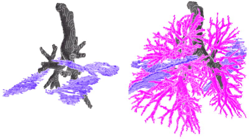
3D renderings of the lung bronchovascular anatomy after refining the voxel-by-voxel classification to form an initial segmentation of airway and airway walls, fissures, and vessels.

4. DISCUSSION

The results presented in this paper show the potential of using of a single approach for the classification of lung bronchovascular anatomy. The classification is intended to serve as an input to more advanced algorithms for the final segmentation. An understanding of the features, feature space, feature selection, dataset, and classifier performance at a fundamental level not only contributes to the field of medical image analysis but may also offer insights to the computer vision community for an application of multiclass classification. The following discussion reviews the methodology and results in more detail in order to provide a thorough understanding of the potential and limitations of this approach.

The simple feature set of attenuation and shape based features was shown to have good performance for differentiating multiple structures. The feature space for the bronchovascular structures presented in Figure 4 corresponds with the a priori expectations for each structure. Even with a good grasp of the feature space, the optimal selection and combination of features is a difficult decision, which is why this process was left to the AdaBoost algorithm. Table 1 suggests that the selected weak classifiers are reasonable based on the feature space. While some classification decisions may appear contradictory, it is likely that with these decisions the algorithm has identified a boundary that provides a relatively low classification error.

Steps were taken to validate the performance and avoid sources of bias; including, having multiple radiologists label a large number of voxels, labeling structures of different sizes, labeling areas of confusion (such as the edge of parenchyma), investigating how the number of weak classifiers impacted performance, and testing on a diverse dataset.

Classifiers were tested independently for comparison with the theoretical AdaBoost performance and enhancement filters. The performance reported in Table 2, indicates the versatility of the feature set and training algorithm even when a limited number of weak classifiers are trained. Qualitatively, the classifier performance appeared to increase with additional weak classifiers as it approached some fundamental limit. Comparison to enhancement filters showed similar or better results. The fissure enhancement method of van Rikxoort and van Ginnekan (2006) also used a pattern recognition technique and a similar feature set. As such, their method is likely to show similar results if applied to multiple structures. Their approach required manual contouring of all fissures in subjects while the method presented in this paper only required the labeling of 150 voxels per structure from each subject. They reported a 0.9044 AUC value for fissure enhancement on a dataset that consisted of 16 scans acquired with 100 to 175 mAs, 0.7 mm thickness, and 16 × 0.75 collimation.

The classifier AUC values were derived from equal numbers of sample voxels from each anatomic structure. When analyzing the whole lung, the number of voxels of each structure will be different, and as such, Table 3 and Figure 5, are better indicators of performance for the whole lung. The results for the multiclass classification presented in Table 3 are more informative of where misclassifications are likely to occur and correlate with the results illustrated in Figure 5. Airways are confused with edge parenchyma, likely due to the airway like appearance of parenchyma near the edge of structures. Fissures are confused with open parenchyma which is reasonable since fissures are faint and distant from nearby structure. Nodules and vessels are commonly confused, which is likely due to branch points, which may appear less tubular and more blob like.

Figure 5.

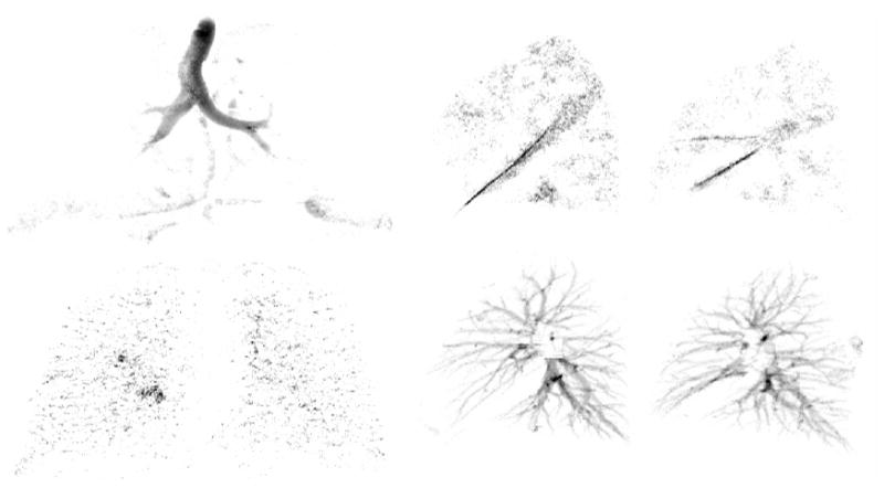
Projection of the airway and nodule classification onto the coronal plane (top and bottom left images), respectively. Projection of the classified fissures and vessels in the left and right lungs onto the sagittal plane (top middle-right) and (bottom middle-right), respectively. The output offers promising results for input to advanced segmentation methods.

The use of cases acquired with a range of imaging protocols for training and testing suggests the robustness of the method. Using attenuation and shape features, computing features over multiple scales, and training on multiple protocols was intentionally done to increase the robustness of the classifier for changing imaging protocols. The average slice thickness of our dataset was 2.3 mm. The method is likely to perform better on thinner images, were there would be less partial volume averaging of structures. While better performance would likely be achieved if the classifier was trained for a single protocol, this is impractical for clinical applications that will receive data from multiple scanners.

Limitations to this study include testing on cases with little or no lung disease, which may confuse the classifiers when encountered. The range of nodule characteristics may also influence the classifier performance. This method is unlikely to detect partial or incomplete fissures. However, determining points along incomplete fissures is an advanced task that requires knowledge of the vascular and airway tree structures. Detecting visible portions of the fissure along with airways and vessels allows further analysis to determine if the fissure is incomplete, and if so, where the fissure boundary should be located. Once segmentation of the airways, fissures, and vessels is complete, a more thorough algorithm could be used for detecting nodules and diffuse lung disease. Future work could also be done to investigate the usefulness of the current feature set for diffuse lung disease classification.

The voxel-by-voxel classification will need to be post-processed to form a final segmentation. However, our intent is to implement advanced techniques that can also remain generic, relying not on structure specific algorithms, but rather a structure specific model learned from contoured data. In this paper, a generic approach (applicable to multiple structures) was presented for use as input to another generic method, such as a deformable model or level set technique, which have the potential to segment various shaped structures (Cootes et al. 1995; Malladi et al. 1995; McInerney and Terzoplolous, 1996; Zhu and Yuille, 1996). In this type of framework, two generic methods (classification and a final segmentation) will be able to perform the function of several specialized methods. As such, this work should be seen as a stepping stone to the final segmentation.

5. CONCLUSION

In this paper, an approach for voxel-by-voxel classification of airway, fissure, nodule, and vessel structures was presented that utilized a small but powerful feature set and showed promising results on a diverse dataset. The AdaBoost algorithm automated the selection of relevant discriminative features for classification and reduced the reliance on a priori knowledge in the feature selection process.

While additional weak classifiers, advanced classification methods, additional examples of misclassified points, and training classifiers for specific imaging protocols may improve performance, it is important to remember, that the overall aim at this stage is not a perfect classification but a simple and robust classification strategy for multiple structures that can be used as input to higher level methods. Future work will be to develop advanced techniques that incorporate anatomical knowledge and imaging physics to refine the voxel-by-voxel classification and provide a thorough analysis for pulmonary disease.

References

- Agam G, Armato SG, III, Wu C. Vessel tree reconstruction in thoracic CT scans with application to nodule detection. IEEE Trans Med Imaging. 2005;24(4):486–499. doi: 10.1109/tmi.2005.844167. [DOI] [PubMed] [Google Scholar]
- Armato SG, III, Giger M, MacMahon H. Automated detection of lung nodules in CT scans: preliminary results. Med Phys. 2001;28:1552–1561. doi: 10.1118/1.1387272. [DOI] [PubMed] [Google Scholar]
- Brown MS, McNitt-Gray MF, Mankovich NJ, Goldin JG, Hiller J, Wilson LS, Aberle DR. Method for segmenting chest CT image data using an anatomical model: Preliminary results. IEEE Trans Med Imaging. 1997;16(6):828–839. doi: 10.1109/42.650879. [DOI] [PubMed] [Google Scholar]
- Brown MS, Goldin JG, Suh RD, McNitt-Gray MF, Sayre JW, Aberle DR. Lung micronodules: automated method for detection at thin-section CT-initial experience. Radiology. 2003;226:256–262. doi: 10.1148/radiol.2261011708. [DOI] [PubMed] [Google Scholar]
- Brushberg J, Seibert J, Leidholdt E, Jr, Boone J. The Essential Physics of Medical Imaging. Lippincott Williams, & Wilkins; Philadelpha: 2002. [Google Scholar]
- Cootes T, Taylor C, Cooper D, Graham J. Active shape models – their training and application. Computer Vision and Image Understanding. 1995;61(1):38–59. [Google Scholar]
- Fiebich M, Wiethold C, Renger B, Armato S, III, Hoffmann K, Wormanns D, Diederich S. Automatic detection of pulmonary nodules in low-dose screening thoracic CT examinations. Proc SPIE. 1999;3661:1434–1439. [Google Scholar]
- Florack L, ter Haar Romeny B, Koenderink J, Viergever M. Scale and the differential structure of images. Imag and Vis Comp. 1992;10(6):376–388. [Google Scholar]
- Food and Drug Administration. Critical Path Opportunities List. 2006 http://www.fda.gov/oc/initiatives/criticalpath/reports/opp_list.pdf.
- Frangi A, Niessen W, Vincken K, Viergever M. Multiscale vessel enhancement filtering. Medical Image Computing and Computer-Assisted Intervention, Lecture Notes in Computer. Science. 1998;1496:130–137. [Google Scholar]
- Freund Y, Schapire RE. A decision-theoretic generalization of on-line learning, and an application to boosting. Journal of Computer and System Sciences. 1997;55(1):119–139. [Google Scholar]
- Krissian K, Malandain G, Ayache N, Vaillant R, Trousset Y. Model Based Detection of Tubular Structures in 3D Images. Computer Vision Image Understanding. 2000;80:130–171. [Google Scholar]
- Lindeberg T. Scale-Space Theroy in Computer Vision. Kluwer Academic Publishers; Dordrecht, Netherlands: 1994. [Google Scholar]
- Lung Image Database Consortium. LIDC Release 0001. 2006 ftp://ncicbfalcon.nci.nih.gov/lidc/LIDC_Release_0001 (since moved to https://imaging.nci.nih.gov/ncia/)
- Malladi R, Sethian J, Vemuri B. Shape modeling with front propagation: a level set approach. IEEE Trans Pattern Analysis and Machine Intelligence. 1995;17(2):158–175. [Google Scholar]
- McInerney T, Terzopolous D. Deformable models in medical image analysis: a survey. Medical Image Analysis. 1996;1(2):91–108. doi: 10.1016/s1361-8415(96)80007-7. [DOI] [PubMed] [Google Scholar]
- Ochs R, Kim H, Angel E, Panknin C, McNitt-Gray M, Brown M. Impact of LIDC reader agreement on the reference dataset and reported CAD sensitivity. Proc SPIE. 2007:6514–82. [Google Scholar]
- Palágyi K, Tschirren J, Hoffman EA, Sonka M. Quantitative analysis of pulmonary airway tree structures. Comput Biol Med. 2005 July 30; doi: 10.1016/j.compbiomed.2005.05.004. [DOI] [PubMed] [Google Scholar]
- Park W, Hoffman EA, Sonka M. Segmentation of intrathoracic airway trees: A fuzzy logic approach. IEEE Trans Med Imag. 1998;17(4):489–97. doi: 10.1109/42.730394. [DOI] [PubMed] [Google Scholar]
- Pizer S, Gerig G, Joshi S, Aylward S. Multiscale medial shape-based analysis of image objects. Proc of the IEEE. 2003;91(10):1670–1679. [Google Scholar]
- Pock T, Janko C, Beichel R, Bischof H. Multiscale medialness for robust segmentation of 3D tubular structures. Proceedings of the Computer Vision Winter Workshop 2005 2005 [Google Scholar]
- Saita S, Yasutomo M, Kubo M, Kawata Y, Niki N, Eguchi K, Ohmatsu H, Kakinuma R, Kaneko M, Kusumoto M, Moriyama N, Sasagawa M. An extraction algorithm of pulmonary fissures from mutli-slice CT image. Proc SPIE. 2004;5370:1590–1597. [Google Scholar]
- Sato Y, Nakajima S, Shiraga N, Atsumi H, Yoshida S, Koller T, Gerig G, Kikinis R. Three-dimensional multi-scale line filter for segmentation and visualization of curvilinear structures in medical images. Med Image Anal. 1998;2(2):143–168. doi: 10.1016/s1361-8415(98)80009-1. [DOI] [PubMed] [Google Scholar]
- Schapire R. MSRI Workshop on Nonlinear Estimation and Classification. Berkeley, CA; 2001. The boosting approach to machine learning: an overview. [Google Scholar]
- van Rikxoort E, van Ginnekan B. A pattern recognition approach to enhancing structures in 3D CT data. Proc SPIE. 2006;6144:61441O. [Google Scholar]
- Wiemker R, Bülow T, Blaffert T. Unsupervised extraction of the pulmonary interlobar fissures from high resolution thoracic CT data. Computer Assisted Radiology and Surgery Berlin 2005. 2005:1121–1126. [Google Scholar]
- Viola P, Jones M. Rapid object detection using a boosted cascade of simple features. IEEE CVPR. 2001;(1):I-511–I-518. [Google Scholar]
- Zhang L, Hoffman E, Reinhardt J. Atlas-driven lung lobe segmentation in volumetric X-Ray CT Images. IEEE Trans Med Imaging. 2006;25(1):1–16. doi: 10.1109/TMI.2005.859209. [DOI] [PubMed] [Google Scholar]
- Zhou X, Hayashi T, Hara T, Fujita H, Yokoyama R, Kiryu T, Hosi H. Automatic recognition of lung lobes and fissures from multi-slice CT images. Proc SPIE. 2004;5370:1629–1633. [Google Scholar]
- Zhu S, Yuille A. FORMS: A flexible object recognition and modelling system. Int J Comput Vision. 1996;20(3):187–212. [Google Scholar]