A biomagnetic system for in vivo cancer imaging

Abstract

An array of highly sensitive biomagnetic sensors of the superconducting quantum interference detector (SQUID) type can identify disease in vivo by detecting and imaging microscopic amounts of nanoparticles. We describe in detail procedures and parameters necessary for implementation of in vivo detection through the use of antibody-labelled magnetic nanoparticles as well as methods of determining magnetic nanoparticle properties. We discuss the weak field magnetic sensor SQUID system, the method of generating the magnetic polarization pulse to align the magnetic moments of the nanoparticles, and the measurement techniques to measure their magnetic remanence fields following this pulsed field. We compare these results to theoretical calculations and predict optimal properties of nanoparticles for in vivo detection.

1. Introduction

Magnetic nanoparticles are a class of particles with diameters of a few to several hundred nanometres (nm) possessing special magnetic characteristics. They normally consist of ferromagnetic cores containing iron, cobalt or nickel but also may include the rare earths. The most typically used particles contain magnetite (Fe₃O₄) or maghemite (Fe₂O₃). Depending upon the size distribution of the nanoparticles, their magnetic properties and the temperature, an aggregate of these single domain ferromagnetic nanoparticles may exhibit an exceedingly strong paramagnetic behaviour: superparamagnetism. Such magnetic nanoparticles behave as free paramagnetic particles in a solution without attracting each other, but, when an external field is applied, their very large intrinsic ferromagnetic moments allow them to polarize easily to form collectively small magnets, approaching ferromagnetic strength.

One can take advantage of this behaviour for in vivo imaging of cancer, tumours or other specific physiological targets. If the nanoparticles are coated with agents that specifically bind to certain types of cells or internal structures (they are overexpressed for these objects), they may be injected into the body without clumping together and are free to circulate until they find their target. They do not display anomalously large magnetic fields until an external magnetic field is applied. At this point they align with the field and display a field typical of ferromagnetic material. When the field is turned off, the nanoparticles exhibit a decaying magnetic field, the remanence field. The remanence field magnitude is strongly dependent upon the magnetic characteristics and the distribution of diameters of the nanoparticles; typically the characteristic time for decay depends on the duration of the polarizing field for a polydisperse size distribution.

This methodology permits the detection and imaging of sub-nanograms of nanoparticles injected into the body for in vivo cancer diagnostics. Injection of magnetic nanoparticles into human beings and animals is a rapidly growing research tool. One major application is in magnetic resonance imaging (MRI) where they are used clinically as contrast agents. Other areas of investigation are magnetic drug delivery enhancement and hyperthermia treatment of tumours. The magnetic separation of specifically labelled cells obtained from serum samples is a well-established tool in biochemistry and cancer laboratories. Magnetic nanoparticles attach to specific cell types by use of special coatings or antibodies. Many types of cancer cells, having specific antigens, can be uniquely targeted by this method. The angiogenesis associated with tumour micro-vascular structure can also be targeted by a variety of angiogenesis agents. A distinct advantage in biomagnetic imaging of nanoparticle sources is the transparency of tissue and bone to low-frequency magnetic fields permitting detection and imaging of nanoparticle sources anywhere within the body. This feature has been well established in magnetoencephalography (MEG) of the brain. The ferrous nature of the nanoparticles is also not a health hazard as they are currently used as MRI contrast agents as opposed to other techniques such as quantum dot technology which contain toxic metals such as selenium, lead and cadmium which could possibly leech out of the nanoparticles.

Biomagnetic sensors have been used in the past for detecting magnetic fields emanating from the body under a variety of conditions. Much of this work is summarized in the review by Andrä and Nowak (1998). One such example is the measurement of biomagnetic susceptibility of liver iron stores where the occurrence of haemochromatosis and thalassemia may be diagnosed (Brittenham et al 1982, Carneiro et al 2002). This is accomplished through the use of a SQUID biosusceptometer. Iron accumulation in the lungs is also measured through a similar technique, magnetopneumography, and is used, e.g., in determining lung damage in miners (Cohen 1973, Nakadate et al 2001). Another application of biomagnetic methods is the measurement of small ingested iron pellets using SQUID sensors through the gut to study motility in gastroenterology (Wenger et al 1957,Baffa and Oliveira 2001).

An extensive body of magnetic nanoparticle research is in the literature (Hafeli et al 1997, Hafeli and Zbrowoski 1999, 2001). Superparamagnetic properties have been well described for such particles (Andrä and Nowak 1998, Landau and Lifschitz 1975) as have the remanence field decays either through Brownian motion for free nanoparticles or through the Nèel mechanism for particles hindered in their ability to rotate because of their attachment to target cells or other objects. The latter typically have much longer remanence times. Kötitz, Romanus, Weber and others (Kötitz et al 1995, 1999, 2000, Weber et al 2001, Romanus et al 2001) have pioneered this field of research. In addition there has been significant work on detecting minute amounts of magnetic material in biological immunoassays (Enpuku et al 2003) and in antibody–bacteria interactions (Grossman 2004). Here, we describe a system using a multi-channel SQUID system designed for imaging the nanoparticles. We also present data showing the magnetic characteristics of certain of these nanoparticles and how they affect the instrumental design.

2. Experimental method

2.1. Sensor system

A very sensitive instrument is required to detect the weak magnetic fields emanating from small clusters of magnetic nanoparticles that have been momentarily magnetized. The instrument must have a detection threshold less than the field emitted by a nanogram or less of magnetized material at a typical distance of 5 cm from the sensor system. Only SQUID sensors are capable of this sensitivity with typical thresholds of 2–5 × 10⁻¹⁵ T Hz^−1/2 for low-temperature SQUIDs (LTS) and near 5 × 10⁻¹⁴ T Hz^−1/2 for high-temperature SQUIDs (HTS). The system used in these experiments was a seven-channel LTS SQUID array originally designed for magnetoencephalography measurements by BTi corporation (BTi 2004). The physical arrangement of the system was a set of second-order gradiometers located with six in a circle of 2.15 cm radius and one at the centre. The baseline of the gradiometer was 4 cm, placing the middle coil at 4 cm and the upper coil of the gradiometer at 8 cm. This system is not optimized for this application.

The system, shown in figure 1, is mounted on a measurement platform consisting of wood with a non-metallic stage for moving samples in the x–y plane. The bottom of the liquid helium dewar is concave with a 16 cm radius of curvature, designed for MEG applications. The distance between the central SQUID and the outside of the dewar was determined to be 1.6 cm by using a small coil and measuring the fall-off of the magnetic field as the coil was moved away from the dewar. No shielding was used for the experiments described here. The SQUID feed-back electronics are able to lock at full gain in this environment due to the presence of the second-order gradiometers. However, because of RF interference on the SQUIDs and the presence of large 60 cycle noise, the performance of the system was limited to ~10⁻¹² T Hz^−1/2. If RF shielding were used to protect the SQUIDs, the noise level would be expected to be ~4 × 10⁻¹⁴ T Hz^−1/2. In a magnetically-shielded room a noise value of 5 × 10⁻¹⁵ T Hz^−1/2 is possible.

Figure 1.

Photograph of system with silicone breast phantom in place.

In order to observe the magnetic signal from the nanoparticles, an external field is applied for a short period. The SQUIDs are turned off during the magnetizing pulse by applying a square wave to the reset control of the feedback electronics. This pulse is sent by the control electronics in the data acquisition computer. It is possible to turn off or on the SQUIDs in less than 1 ms by this method.

The seven-channel SQUID system measures the remanent field emanating from clusters of nanoparticles after the magnetizing field is turned off. In general, six measurements are required to determine the vector components to localize a magnetic source. In the present case, however, for our experimental study, the magnetizing field aligns the nanoparticles along the field axis so that only four measurements are required. The seven-channel system over determines these parameters permitting greater accuracy in localization. Imaging several sources simultaneously would require a larger array of SQUIDs. Inverse theory mathematical formalisms can then be applied to determine the location of the sources (Flynn 1994, Huang et al 1998). We address this question further in section 6.

2.2. Magnetizing the nanoparticles

A cluster of magnetic nanoparticles will produce an observable field only when their magnetic moments are aligned (magnetized) by relaxing in the direction of an externally applied magnetic field. The duration of the applied field must be compatible with the characteristic relaxation times of the particles. When the field is switched off, the moments again lose their alignment as they relax back to random orientations in their characteristic times. The primary method of magnetization uses Helmholtz coils surrounding the measurement chamber as shown in figure 1. This method has been also used extensively by Kötitz et al 1995. A disadvantage of this method is the presence of small induced currents produced in the present SQUID support structure resulting in a background decaying field. Such transients must be subtracted from the nanoparticle results.

The Helmholtz coils (see figure 1) are each 16 mH inductance, 60 cm on a side, with 100 turns of no. 16 magnet wire operating in a parallel mode. A 3 KW current-regulated power supply provides up to 35 A to produce the magnetizing field. The power supply is connected to a special pulsing circuit designed for this purpose. The circuit is controlled by a computer using LabView software (National Instruments, LabView 2004). Our standard procedure is to apply a 1 s, 30 A current pulse, immediately after the current is switched off, measure the remanence flux from the magnetized nanoparticles for 2 s, and repeat this sequence for a pre-determined time depending on the magnitude of the signal being measured. Typically, we use 25 trials. The electronic circuit that turns off the coil rapidly dissipates the energy in the coils. The current is measured using a 50 A shunt and is normally set at 30 A producing a field of 32.8 G at the centre of the measurement chamber where the samples are placed. The quenching time is 1.4 ms with zero observable current in the coils after this point as measured both by the shunt and observing the residual field.

An important feature of the Helmholtz coils is the uniformity of the magnetic field in the vicinity of the SQUID sensors. These sensors are second-order gradiometer types to provide background rejection for uniform fields. The principal reason for this choice of gradiometer over a magnetometer is the rejection of distant sources such as moving metal items, electronic circuits, etc. Moreover, this uniformity offers the additional advantage in reducing the effect of the pulsed Helmholtz field on the sensors. The field uniformity at the sensors is better than 1%.

The magnetizing field produces about 0.54 of the magnetic saturation value of typical ferrite cores which is adequate to provide reasonable magnetization of the samples. New calculations indicate that the pulse duration of the magnetizing field can be reduced to 0.1 s with only a small decrease in the induced magnetization. The principal problem we have encountered is that the SQUID system was not designed to be operated in the presence of a pulsed magnetic field. The components of the SQUID support system contain some metal in which currents can be induced when the Helmholtz coils are switched off. The resulting artefact decaying field can be removed quite well with a sample-out background subtraction. A re-design of the support system could substantially reduce the need for this background subtraction.

2.3. Experimental control

A flexible multitask data-acquisition computer program, based on the programming language LabView, is used to acquire the data and control the pulsing sequence. A data acquisition card is located in the backplane of the control computer. This data acquisition hardware consists of 16 channels of analogue-to-digital conversion, at 16-bit resolution, and 100 k samples s⁻¹. There are also two channels of digital-to-analogue output and eight-digital output channels. Software parameters include the number of active channels, data acquisition rate, number of output channels, pulse length, data acquisition time and number of sequences to take. A low-pass filter to remove noise from the data, such as 60 Hz line noise is used to provide an online display. The online display parameters include gain, offset and time windows for convenient display of the data as they are being acquired. Also displayed is a selected raw data channel as well as an fft frequency spectrum. All of the filtered and raw data for all seven channels, the timing pulses for the reset, the Helmholtz coils and the shunt current are digitized and stored in a spreadsheet file.

The data acquisition sequence is triggered by a software dual-function generator. We acquire 2 s of data at 1000 samples s⁻¹ after a 1 s magnetization pulse. The output triggers from a software function generator initiate the data-acquisition sequence by (1) applying a reset pulse to the SQUID feedback controls, (2) after a short delay, sending a pulse to the Helmholtz-coil-controlling circuit to apply current to the coils, (3) after 1 s, turning off the Helmholtz coils, (4) after several milliseconds removing the SQUID reset pulse, with data acquisition occurring for 2 s. This method is precise to within 0.1 ms, permitting accurate overlap of repeat sequences for the purpose of signal averaging. Typically, we operate the program for 75 000 ms with 25 3 s pulse sequences. The results are then signal-averaged to increase the signal-to-background ratio by a factor of 5. The number of sequences can be increased or decreased by software command to accommodate the remanence field signal strength.

We use a code written in IDL language (Research Systems Inc. 2004) to analyse these data by summing all of the pulse sequences and averaging them. This analysis is also done for the no-sample background run in the same code and any background signal is subtracted. The data are converted from volts to tesla and graphically presented for all seven SQUIDs. The conversion factor was experimentally measured using a coil that produced a known magnetic field at each sensor. An electromagnetic finite element code (Flynn 2004) is used to calculate the exact fields at the sensors taking into account that they are second-order gradiometers and the finite size of the sensor coils.

2.4. Nanoparticle properties

A number of superparamagnetic nanoparticles with various magnetic characteristics were investigated. The nanoparticles chosen have biocoatings that are adaptable for coating with antibodies for specific cancers, angiogenesis agents or other organ-specific molecules. A cartoon of a coated magnetic nanoparticles is shown in figure 2. Nanoparticles from a number of commercial suppliers were selected to explore various properties and remanence time distributions for each type of particle. Nanoparticles were obtained from Bang’s Laboratories Inc. (2004), Spherotech Inc. (2004),Chemicell GmbH (2004) and Miltenyi Biotech Inc. (2004). The Miltenyi nanoparticles we used were already attached to lymphoma cells by antibodies during a cell separation procedure performed in the University of New Mexico Cancer Research and Treatment Center and had been deposited on slides and allowed to dry. These particular slide preparations contained known numbers of cells and nanoparticle sites per cell. Some properties of these nanoparticles are shown in table 1.

Figure 2.

Cartoon of coated nanoparticle.

Table 1.

Properties of nanoparticles used in this study.

Spherotech	~15 nm	CM-10−10 Carboxyl, 1.1 μm hydrodynamic diameter
Bang Labs	Unknown	MC04N DiViny/Benson/V-C004, Mag 41%, 0.7 μm hydro. dia.
Chemicell	~25 nm	SiMAG-1/1411 & −1/1410 30 mg ml−1
Chemicell	~50 nm	FluidMag-GA/2G 75 mg ml−1
Miltenyi	~5–8 nm	With antibodies attached to lymphoma cells

The specialized properties of magnetic nanoparticles have been exploited in a number of research protocols. For example, they have been used in the ultra sensitive detection of proteins (Nam et al 2003). They have been applied in a variety of medical applications such as magnetic cell separation, drug delivery, RF heating of tumours and MRI contrast agents (Pankhurst et al 2003). Mobility measurements of cells and antibody binding have been measured with magnetically labelled cells (Chalmers et al 1999a) as have a variety of cell properties (Chalmers et al 1999b).

We investigated two methods of nanoparticle preparations, slides and injected silicone phantoms, to measure their magnetic parameters and characteristics.

2.4.1. Slides with dried nanoparticle preparations

The simplest of these preparations are measured amounts of nanoparticles in colloidal suspension subsequently dried on slides. These preparations permit definitive measurements of Nèel mechanism parameters because the particles are fixed. In some cases, the preparations were dried in the presence of strong magnetic fields to measure the effects of magnetization on the ‘easy-axis’ of magnetized materials. An assortment of slides was prepared. Amounts ranging from 1 μl to 40 μl were deposited on the slides in ~3 mm diameter wells formed by acrylic, and after drying, the preparations were covered with a thin acrylic layer to protect them. Identical slides were made without nanoparticles and used to measure artefact fields. Measurements confirmed that empty slides themselves did not produce any signal.

Calculations indicate that the ideal range of nanoparticle diameters for remanence measurements in the millisecond to second range is from 20 to 25 nm. The nanoparticles from the various laboratories chosen have a large range of core diameters and permit investigation of a range of nanoparticle characteristics.

2.4.2. Silicone phantoms

To represent better the actual conditions in breast cancer imaging that are present during magnetic in vivo remanence measurements, special phantoms were prepared and injected with nanoparticle suspensions. The most elaborate phantom consisted of a silicone material in the shape of a female breast that had been originally developed for testing mammography devices and for practicing needle biopsies. It has small non-magnetic inclusions to represent tumours or calcifications. The outer skin of the phantom is self-sealing for the needle biopsies making it ideal for directly injecting small amounts of nanoparticleladen fluid into selected sites.

For most experiments, we fabricated phantoms that were silicone molds 85 mm in diameter and about 45 mm deep with the top approximating a hemispheric surface. Figure 1 is a photo of one such phantom under the sensor system. The phantom rests on a non-magnetic, two-dimensional stage that permits movement of the phantom under the sensor system. The phantoms were injected with nanoparticle suspensions at a depth of 16 mm, at the centre of the mold top. Some phantoms had no injections and served as reference background sources. An MRI image of one of the injected silicone phantoms (phantom number P6), containing a 20 μl suspension of ChemiCell nanoparticles, is shown in figure 3. The bright spot at the centre results from the perturbation of the MRI field by the ferromagnetic cores of injected nanoparticles. It is located 15 mm from the top as expected from the position of the injection needle. The dark areas in the phantom arise from air that was trapped in the silicone during fabrication. Other silicone phantoms were injected with nanoparticle suspensions as follows: (phantom P8) 7 μl of Spherotech particles, ~1 × 10⁹ nanoparticles, (phantom P1) ~20 μl of Bang’s Laboratory nanoparticles, and (phantom P2) ~20 μl of Chemicell SiMag-1/1411, ~10¹² nanoparticles. The average diameter of each nanoparticle sample varies with the sample.

Figure 3.

MRI of phantom containing nanoparticles.

3. Results of magnetic remanence field measurements

The magnetic remanence field following a magnetization pulse is determined by the properties of these superparamagnetic, or Stoner–Wohlfarth, particles (Landau and Lifschitz 1975, Andrä and Nowak 1998, Stoner and Wohlfarth 1948) in which the ferrite core is a single-domain particle. After an array of these particles is magnetized briefly by alignment with an external field, which is subsequently removed, the remanent magnetization decays as the alignment reverts to chaos, either by Brownian motion, typically in microseconds, or, if the particle are fixed and cannot rotate freely, by the Néel mechanism, in milliseconds or longer. This behaviour is exploited for cancer-cell detection. Those nanoparticles, attached to tumour cells and unable to physically rotate, will yield an observable magnetic signal milliseconds to seconds in duration whereas free nanoparticles will disorient too rapidly to be observed after the magnetization field is switched off.

A significant additional advantage in this method for antibodies is that typically a large number of antibodies will attach to a cancer cell, meaning that large numbers of properly coated nanoparticles can bind to the cell surface. In the Miltenyi slide, discussed above for lymphocyte cells, 20 000 antibody binding sites per cell were known from cytometry measurements. In some cases, there may be as many as 10⁷ antibodies attached to each cancer cell (Lewin et al 2000). In this case, the cell can be completely tiled with nanoparticles one-layer thick. One can estimate, as shown below, that for typical nanoparticles, approximately 10⁹ particles will produce a field of 10⁻¹³ T at a distance of 5 cm, making it possible to detect clusters of from 10⁴ down to 10² cancer cells depending upon the number of antibody sites and therefore the number of nanoparticles that can bind to each cell.

3.1. Theoretical calculation of field strength

The expected remanence fields can be calculated from a localized source of magnetized nanoparticles using the formula for the field from a dipole:

$$\mathbf{B}(\mathbf{\mu },\mathbf{r})=({\mu }_0/4\pi )\hspace{0.17em}((3(\mu ·\mathbf{r})\mathbf{r})/r^5-\mu /r^3).$$ (1)

For both μ and r along the z-axis, directly under the central SQUID in the seven-channel sensor system, we have simply

$$B_z=({\mu }_0/2\pi \hspace{0.17em})(\mu /z^3)$$ (2)

where B and B_z are magnetic flux densities in tesla, μ is the magnetic moment in units of A m², r is the distance from source to sensor. The value of μ is just Nμ_p, where N is the number of nanoparticles in the localized source and μ_p is the average projection (assuming here that the Langevin function, discussed in section 5, is reasonably close to unity) of the nanoparticle dipole moment along the total magnetic dipole direction. For a ferromagnetic nanoparticle of diameter d and spontaneous magnetization M_s (units of A m⁻¹ or J T⁻¹ m⁻³), the permanent magnetic dipole moment is

$${\mu }_p=M_{\mathrm{s}}(4\pi /3)\hspace{0.17em}{(d/2)}^3.$$ (3)

There are only a few examples given in the literature of values for μ_p, magnetization saturation and particle diameter. Keller et al (2000) have provided an excellent study of one such nanoparticle identified as NC100150. The values reported were μ_p= 4.38 × 10⁻²⁰ A m² (or J T⁻¹) and a diameter, d, of 6.43 nm, maghemite (Fe₂O₃) single-domain crystal. In order to estimate the detectability of these nanoparticles, we assume a reasonable sensitivity of the SQUID to be 1 × 10⁻¹³ T (100 fT). To produce this field with a source of nanoparticles of the type described above with the source at a distance of 5 cm, using equation (2), would require a quantity of 1.4 × 10⁹ nanoparticles, a mass of ~0.7 ng of iron. We must point out that, as we shall discuss below, these small-diameter particles would have relaxation times, Néel as well as Brownian, much too small for observation by our techniques.

3.2. Theoretical calculation of remanence field and comparison to data

The remanence field data from polydisperse magnetic nanoparticle samples can be fit with a formula due to Nèel (1949) yielding a logarithmic decay of the field with time after the switching off the polarizing field. This formula works well when the time is small compared with the duration of the polarizing field. A more general formula was derived by Chantrell et al (1983), where the argument of the logarithm is 1 + t₀/t, where t₀ is the duration of the magnetizing pulse and t is the time since the turn-off. The decays we have studied are primarily due to the Nèel mechanism but may also be influenced by Brownian motion in some conditions. A general formula for fitting the data can thus be given by

$$F=a_0+a_1\ln (1+a_2/t)+a_3\sin (a_4+a_{5}t)+a_6\hspace{0.17em}\exp (-a_{7}t).$$ (4)

In this equation (1) a₀ has no physical significance and represents an arbitrary (offset) static field since a SQUID is designed to measure only changes in fields, (2) a₁ parametrizes the remanence field and depends on the overall magnetic moment of the source that reflects the number and size distribution of particles, their magnetization, and the characteristics of their ferrite cores, (3) a₂ is a time parameter, theoretically expected to be the pulse duration of the magnetizing field, t₀, which in the present case is 1000 ms, (4) a₃ is the amplitude of any sinusoidal contaminant in the data, which will be normally 60 cycle that had not been completely removed either through the low-pass filters or the signal averaging, (5) a₄ is the phase shift of this sinusoidal component, (6) a₅ is the angular frequency which has been determined to be primarily 60 Hz (if other frequencies are present they can be fit separately), (7) a₆ is the amplitude of any Brownian or other exponential contribution to the decay of the magnetic data, and (8) a₇ is the decay constant of the exponential term. In general, the trend of the data is well fit by the first two terms of this equation with the third term simply fitting the superimposed 60 Hz component. The exponential term usually has little effect beyond increasing parametrization of the fit.

This equation was used to fit the data using a Levenberg–Marquardt algorithm for nonlinear least square fitting. The algorithm was incorporated into a code written in IDL language. The code was arranged so that any parameter could be held fixed or varied as desired. In results presented below, the data, the theory and the difference between theory and data are shown. The fits, in general, are quite good except at the earliest times. The addition of the 60 Hz component of the fit does reduce somewhat the noise in the residuals but has no effect on the trend. The addition of the exponential term is not important in dried slide preparations, and is normally omitted for slides, but does show some improvement in the injected phantoms.

3.2.1. Experimental results for dried preparations on slides

Figure 4 shows the remanent magnetic field versus time for slide S1 with leukocyte cells labelled with magnetic nanoparticles. This slide contains a known number of cells with a known number of nanoparticles per cell based on cell cytometry counts. The cells were obtained from a bone marrow sample taken during a leukaemia biopsy. The serum from the biopsy was mixed with magnetic nanoparticles coated with specific antibodies for lymphocyte cells (white blood cells). The nanoparticles bound to the cells at a count of ~2 × 10⁴ per cell, and the mixture was then passed through a magnetic separation column (MACS) to sort out the labelled cells from the rest. The cells were then further identified and placed on a slide to dry. From the cytometry measurements, there are 4.8 × 10⁷ cells with 2 × 10⁴ nanoparticles/cell, giving a total of 9.7 × 10¹¹ nanoparticle sites on the slide. In figure 4, there is a 30 ms delay between the end of the field pulse and the first of the data due to an induced signal in the SQUIDs at this high gain of 1000. The signal is clear and at least an order of magnitude larger than the background noise. The formula given in equation (4) is used to fit these data and is also shown in figure 4. The lower curve is the difference between measured data and fit. The parameters from this fit are included in table 2 (S1 Miltenyi). These nanoparticles from Miltenyi are available with a large variety of antibodies and other agents. As we show below, we are able to use these measurements and the cell count to establish an average magnetic dipole moment for these nanoparticles. Unfortunately, there is little published information on their magnetic properties.

Figure 4.

Remanence fields for slide with leukocyte cells.

Table 2.

Parameters from equation (5) for four slide preparations used in this study. The parameters a₀, a₁, a₆ are in tesla, a₂ is in millisecond, a₇ is in ms⁻¹.

Sample	a0	a1	a2	a6	a7
S1 Miltenyi	−2.38 × 10−11	1.42 × 10−11	1000	0.0	0.0
S3 FluidMag	−1.60 × 10−11	3.52 × 10−10	1000	5.89 × 10−10	0.099
S5 Bang’s	3.17 × 10−11	1.86 × 10−11	1000	8.25 × 10−11	0.021
S12 Spherotech	−1.50 × 10−10	1.80 × 10−10	1000	0.0	0.0
S19 SiMag	−9.24 × 10−10	1.18 × 10−9	1000	0.0	0.0
S31 SiMag	−2.1 × 10−11	2.5 × 10−11	1000	0.0	0.0

Figure 5 presents examples of remanence magnetization for the four nanoparticle types given in table 1. The measured magnetic fields are in teslas, with an arbitrary offset, since SQUIDs respond only to changes in field. The results shown in figure 5 are also compared to equation (4). The data were obtained with larger quantities than shown in figure 4 with the purpose of determining various nanoparticle characteristics. Different particle types with different size distributions produce a considerable difference in amplitude although, except for monodisperse populations, the time to baseline remains the same. This variation in amplitude is due to a number of factors such as nanoparticle amounts on the slide, the size distribution and the magnetic characteristics of the nanoparticles. The magnetic characteristics can be approximated from other published results. There is substantial dispersion in nanoparticle size among each sample, but our system responds to only a relatively narrow band of sizes, as we shall discuss below. These observations can be used to extrapolate results to shorter times after the magnetizing pulse since the current SQUID system does not reach an equilibrium value for magnetic field until 10–40 ms after the reset is released due to transient fields generated from eddy currents in the metallic components in the SQUID supporting column. Table 2 contains the parameters for a number of slide sample fits to equation (4)

Figure 5.

Remanence fields for four nanoparticle types of table 1.

The data presented in figure 5 were obtained at a SQUID gain of 10, which corresponds to 1.5 × 10⁻⁸ fT V⁻¹, using a conversion factor obtained from a known current source. Data in figure 6 were obtained at a gain of 1000 where the conversion factor is 1.4 × 10⁻¹⁰ fT V⁻¹. In the higher gain mode, remanence fields for >1 μl suspensions of these sample nanoparticles in figure 5 are observed.

Figure 6.

Remanence fields from three different phantom sources.

We use equations (2) and (3) to extract magnetic parameters for some of our nanoparticles. The nanoparticles for the S31 sample, included in table 2, are Chemicell SiMag-1/1411nanoparticles with a hydrodynamic diameter of 75 nm (no biocompatible coating). A sample of these nanoparticles, about 7 μl in solution, was placed on a microscope slide and dried. The number of nanoparticles is estimated to be ~3 × 10¹¹ and the average diameter of the nanoparticle is ~25 nm. The remanence field from equation (4), when extrapolated to 1 ms, is a field B_z of 1.7 × 10⁻¹⁰ T (using the parameters a₁ and a₂). The distance from slide to sensor was 25 mm, resulting in a predicted total magnetic dipole moment, μ, of 1.4 × 10⁻⁸ J K ⁻¹. For the same magnetization as reported by Kellar et al (2000)μ_p would be ~(25/6.4)³ × 4.4 × 10⁻²⁰ = 2.6 × 10⁻¹⁸ J T⁻¹ and since μ = Nμ_p, the predicted N is 5.4 × 10⁹. However, the nanoparticles used here were magnetized in a field of 3.28 × 10⁻³ T. Examining the Langevin function for magnetization of these assumed maghemite particles, this field would produce ~54% of the magnetization of the saturated field. Consequently we can estimate that the value of N increases to about 10¹⁰. This is in reasonable agreement with the volume estimate for the number of nanoparticles on the slide, since the distribution could be quite broad, with only those in a narrow size interval having relaxation times in the range required to be detected.

3.2.2. Phantom results

Figure 6 is a comparison of three different nanoparticle preparations injected into the silicone phantoms shown in figures 1 and 3. The curve in the middle on the right-hand side of the plot is using nanoparticles from Chemicell, the lowest curve is using particles from Spherotech and the upper curve is from a phantom using particles from Bang’s Laboratories (the Bang nanoparticle data are much weaker than the other nanoparticles and have been multiplied by 10 for comparison on the same plot). The injected nanoparticles for these phantoms consisted of (1) 7 μl of Spherotech particles, CM-10-10 Carboxyl 2.5% w/v 1.5 g cm⁻³ hydrodynamic diameter = 1.1 μm, (2) ~20 μl of Bang’s Laboratory MC04N P S nanoparticles with diveny/benson/v-coooh/mag coatings with a mean hydrodynamic diameter of 0.7 μm, and (3) ~20 μl of Chemicell SiMag-1/1411nanoparticles with a hydrodynamic diameter of 75 nm. The approximate number of nanoparticles injected for case (1) is ~1 × 10⁹. The number for case (3) injected is ~10¹² with the number for case (2) being uncertain. The average diameter of the nanoparticle ferromagnetic core varies for each nanoparticle with case (1) ~15 nm, (2) ~5 nm, (3) ~25 nm. How these nanoparticles are fabricated and how the magnetically active sites are distributed in the particle itself may have a very large effect upon the remanence fields measured in this method.

The first sample considered in table 3 is an injected phantom containing 40 μl of solution and allowed to dry in the silicone phantom. The phantom was injected at a depth of 16 mm and pressed against the bottom of the dewar giving a total distance to the sensor similar to that of the slide preparation (25 mm). The expected ratio of magnetic source moments is the ratio of the volumes of solution allowed to dry, 40 μl for the phantom versus 7 μl for the slide, giving a ratio of 5.7. The observed ratio of phantom versus slide remanence field magnitudes, using parameter a₁ in fitting the data, is 6.8. This is considered as reasonable agreement in estimating the number of injected compared to dried nanoparticles in the phantom and slide preparations. These estimates of the number of nanoparticles that produce the observed magnitude of the remanence field are essential in an in vivo study in determining the physical character of a lesion.

Table 3.

Parameters from equation (5) for three phantom preparations used in this study. The fit was done using the log and exponential term as well as for any sinusoidal component. Same dimensions as in table 2, with a₄ unitless and a₅ in ms⁻¹. The fits for P6* and P1* were done without the exponential term for comparison.

Sample	a0	a1	a2	a3	a4	a5	a6	a7
P6	−1.6 × 10−11	1.7 × 10−10	1000	−1.1 × 10−12	−3.92	0.377	−1 × 10−12	0.014
P6*	−1.5 × 10−10	1.6 × 10−10	1000	−1.0 × 10−12	−3.98	0.377	0.0	0.0
P1	+6.6 × 10−12	2.3 × 10−11	1000	−9.9 × 10−13	1.59	0.377	7.7 × 10−11	0.057
P1*	+3.4 × 10−12	2.7 × 10−11	1000	−1.0 × 10−12	1.69	0.377	0.0	0.0
P8	−1.3 × 10−9	1.5 × 10−9	1000	+8.2 × 10−13	−2.87	0.377	−3.3 × 10−9	0.014

Theoretical fits to the silicone phantom data are improved by the addition of the exponential term. Resulting fit parameters for three phantoms are given in table 3 where a comparison is made with and without the exponential term for two of these cases. These results indicate that the nanoparticle solution has different characteristics within the silicone phantom than dried upon the slide. This may be due to either the preparation remaining partially liquid or the adherence to the walls of the silicone enclosure created during the injection being different than on the slide. An over- or under-abundance of particles of a certain relaxation time in the nanoparticle size distribution could also result in the addition of a positive or negative exponential term, respectively. An improvement in chi-squared values by a factor of ~2 is obtained by including the exponential for the phantom whereas no change in chi-squared was observed in the slide preparation.

4. Pre-magnetizing the magnetic nanoparticles

We examined whether the magnetic remanence fields would be affected by orientation of the magnetic ‘easy axis’ of the nanoparticle single-domain crystals. Measurements were made to determine some of the elements of the physics of the magnetization process with the goal of potential enhancement of the remanent signal from these nanoparticles.

Two different types of nanoparticles in colloidal suspension were placed, while drying on the slides, in the 5 kG field of a C-magnet consisting of two Nd–Sm–Co magnets on the pole faces of a soft-iron magnet. The slides were arranged to have the field direction perpendicular to their surface—the ‘aligned condition’—or parallel to the slide surface—the ‘tangential position.’ Each sample was placed in the magnet immediately upon deposition of the nanoparticle suspension on the surface and remained there until completely dried. They were then coated with a non-magnetic acrylic coating to assure stability of the material. Remanence measurements were taken at numerous times to determine if particle alignment changed as a function of time. Two samples of quite different average sizes were used, one containing 20 μl of ~15 nm diameter nanoparticles, and the other 7 μl of ~25 nm.

In figure 7, the results of the measurements on the smaller diameter (Spherotech) nanoparticle are shown. Three samples were used; one was magnetized perpendicular to the slide face, one tangential, and the other dried outside of the field. The uppermost curve in figure 7 is from the aligned sample and the two lower data sets are from the tangential magnetization and the non-magnetized samples. The latter two are basically indistinguishable and overlap. Since the measured magnetic field is relative because it includes arbitrary offsets, all of the three samples have been set equal at approximately 2 s after the Helmholtz pulse was turned off. The data are shown from 20 ms after the pulse to 1970 ms after. The results indicate significant effects of pre-magnetization and the importance of aligning the easy axis with the subsequent direction of the magnetizing field of the Helmholtz coils. The aligned condition has a substantially different remanence field characteristic than the tangential and the non-magnetized, the latter two being essentially equivalent. This difference reflects the presence of a larger magnetic moment for the collection of nanoparticles after the application of the pulsed polarizing field when the particles are fixed with their easy axis in the same direction as this field. This pre-orientation of the individual dipoles may affect the relaxation times or it may increase the effective torque on the dipoles when the polarizing field is applied. Because of this, the electronic structure of the magnetic core may require less energy to align during the presence of the polarizing field resulting in a larger moment. We have fit these data using the theory outlined above, and table 4 contains the results for the effective moment parameter, a₁, for these three cases.

Figure 7.

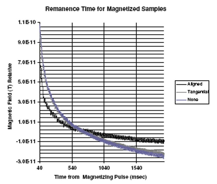
Effects of pre-magnetization on 15 nm nanoparticles.

Table 4.

A comparison of the relative strengths of the remanence fields, using the a₁ parameter, for different pre-magnetization alignments. (See the text for definitions.)

Sample (nm)	Φr Aligned (T)	ΦrTangential (T)	ΦrNone (T)
Sample 1, ~15	4.3 × 10−11	1.25 × 10−11	2.0 × 10−11
Sample 2, ~25	2.3 × 10−11	4.5 × 10−11	4.5 × 10−11

The second sample, consisting of larger nanoparticles (Chemicell), was pre-magnetized in the 5 kG field in the opposite direction to the polarizing field of the Helmholtz coils. The quantity of fluid dried on the slide was approximately one-third of the previous sample but, probably the larger average size of these particles means more are in the size range to be detected. The larger particles produce a larger signal, and the remanence field magnitudes are similar to those shown in figure 7. Again the tangentially pre-magnetizing field and no field give approximately identical remanence field behaviour. The theoretical fit values are also given in table 4. In this case, the aligned field produces a substantially reduced remanence field signal compared to the others as one might expect from the anti-alignment. The ratio of the values of Φ_r for the aligned smaller diameter sample is 3.44, whereas the ratio for the larger anti-aligned sample is 0.51. These results indicate that pre-polarization can produce a substantial change in the remanence fields, consistent with the field being in alignment with the polarizing pulse and indicative of an important ‘easy magnetic axis’ dependence of the magnetic moment. There is clearly a need for further study of this phenomenon.

5. Theoretical predictions for optimal nanoparticle diameters

The measurements we have discussed above require that the particles under study must align with the applied field in a time of the order of the duration of the applied field. When the field is switched off, they must maintain their remanent magnetization for a time also of the order of this duration down to a few tens of milliseconds. For shorter decay times the signal becomes obscured by instrumental transients. Except for free nanoparticles with very large hydrodynamic radii, the Brownian relaxation times are much too short to show up in our observations. We therefore are sensitive only to magnetic nanoparticles that are bound; they can reorient only via the Nèel mechanism (Nèel 1955). That is, the collective alignment of the unpaired electrons that contribute to the magnetism rotates, although the crystal itself remains fixed. The associated relaxation time is a remarkably strong function of the size of the nanoparticle. As a consequence only a very small range of diameters are useful in the time interval selected for the measurements.

The relaxation time τ_N is usually taken as

$${\tau }_N=C\exp \hspace{0.17em}(KV/kT),$$ (5)

where C is a constant, often taken as 1 ns, as we do in examples discussed here, K is the magnetocrystalline anisotropy energy per volume, V is the volume of the single domain, k is Boltzmann’s constant, and T is the absolute temperature. We form an expression first for the remanent polarization of a monodisperse collection of N nanoparticles each of volume V. We polarize them for a time t₀ in a magnetic field. Immediately upon turning the field off, we have a collective magnetic moment of

$${\mu }_0=N{J}_{\mathrm{s}}VL(x)\hspace{0.17em}\{1-\exp (t_0/{\tau }_N)\},$$ (6)

where L(x) is the Langevin function, with x = J_sV B/kT, with B the applied magnetic flux density and J_s is the spontaneous magnetization of the ferromagnetic substance of the nanoparticle (magnetic dipole moment per unit volume, A m⁻¹). Subsequently, measuring t from the instant of switch-off of the field, we have for the remanent dipole moment of the collection of monodisperse particles,

$$\mu (t,V)={\mu }_0\exp (-t/{\tau }_N).$$ (7)

Now let us consider a polydisperse collection described by a lognormal distribution of radii of the magnetite cores of the nanoparticles, given by

$$P(r)=\frac{1}{r\sigma \sqrt{2\pi }}\exp \left(\frac{{-(\ln \hspace{0.17em}r-m)}^2}{2{\sigma }^2}\right),$$ (8)

where the rather arbitrary parameters are given in table 5. For simplicity we have taken the nanoparticles to be spherical, so that V = 4π r³/3. In figure 8 we show the distribution of magnetic moment as a function of radius for several values of t. The remanent magnetic moment of the ensemble as a function of time then can be written as

Table 5.

The symbols, values and units used in the theoretical calculations.

Nanoparticle features	Symbol	Value	Units (all SI)
Material	Magnetite (Fe3O4)
Spontaneous magnetization	I	4.72 × 105	J T m−3
Field strength	B	0.003 28	T
Temperature	T	310	K
Boltzmann constant	k	1.38 × 10−23	J K−1
Permeability of free space	μ0	4π × 10−7	SI
Anisotropy energy density	K	1.34 × 104	J m−3
Peak of lognormal distribution	m	ln(11)	Argument is radius in nanometer
Standard deviation of lognormal distribution	σ	0.20	Unitless

Figure 8.

Effective magnetic moment for times after the termination of the magnetizing pulse as a function of the particle radius.

$$\mu (t,t_0)={\int }_0^{\infty }\hspace{0.17em}P(r)\hspace{0.17em}{\mu }_0\hspace{0.17em}(r,t_0)\hspace{0.17em}\exp \hspace{0.17em}(-t/{\tau }_N)\hspace{0.17em}\mathrm{d}r.$$ (9)

The remanent magnetic dipole moment turns out to be well approximated, just as Chantrell et al (1983) have shown, at larger t by

$$\mu \hspace{0.17em}(t,t_0)=A\hspace{0.17em}{\ln (1+t}_0/t).$$ (10)

Figure 9 displays the result of a numerical integration showing the integral result and the fit of equation (10) to the data.

Figure 9.

Average remanent dipole.

As has already been pointed out, the characteristic time of the remanent magnetization for the integral over a relatively broad distribution of nanoparticle radii is just the time of magnetization t₀. The ensemble of nanoparticles can ‘remember’ how long they had been subjected to the polarizing field. An individual particle cannot ‘remember’ because it just follows its characteristic relaxation time. The behaviour of the ensemble, on the other hand, is modelled by an integration over the individual relaxation times; the only time remaining free in the model then is just the time of application of the field, t₀.

For purposes of optimizing the experimental parameters for cancer detection, it is useful to examine some of the ‘active ingredients’ in equation (6). For simplicity, let us study the behaviour of the product of the last two terms in equation (6). In figure 10 we display the dependence of L(x) {1 − exp(t₀/τ_N)} on the particle radius for several different values of the time t₀ of application of the polarizing field. We see that t₀ can be diminished considerably without appreciably decreasing the response. Factors of 10 increase in the data-taking rate are possible over our present rate by shortening t₀.

Figure 10.

The fraction of saturation, L(x){1 − exp(t₀/τ_N)}, reached on the average by a given nanoparticle with a magnetite core of radius r is shown for a magnetizing field of 32.8 × 10⁻⁴ T with various durations of application. These results indicate that our technique can be made much more efficient if the pulse duration is reduced.

Likewise, what is the effect of the strength of the polarizing field? From figure 11 L(x) {1 − exp(t₀/τ_N)} is displayed as a function of the particle radius for several different values of the polarizing field. Figure 12 shows the peak values versus field strength. Saturation corresponds to L(x){1 – exp(t₀/τ_N)} = 1. The field we used in our measurements, 32.8 G, is about 56% of saturation. And one can see at this field we are quickly approaching the point of diminishing returns.

Figure 11.

The fraction of saturation, L(x){1 − exp(t₀/τ_N)}, reached on the average by a given nanoparticle with a magnetite core of radius r is shown using a magnetizing pulse duration of 1 s for various strengths of the magnetizing field.

Figure 12.

The peak fractions of saturation for various field strengths shown in figure 13 plotted versus the field strength. We see that our signal can be increased by increasing the field strength, but that we are nearing the point of diminishing returns at around 50 G.

6. Imaging of sources

There is a distribution of remanence field amplitudes across all of the sensors in the seven-channel system due to the spatial distribution of the SQUIDs within the dewar. This information is used to localize and image the nanoparticle source using an algorithm involving a least-squares approach to model the electromagnetic inverse problem. In order to obtain an experimental verification of the spatial accuracy for imaging sources, we performed a complete mapping of SQUID response over a grid of ±10 cm centred around the central SQUID and 50 mm below the dewar using one of our phantom sources. There are two surfaces to consider in these measurements: one is the surface containing the sensors and the other contains the sources, in this case, the stage containing the phantom. The relative orientation of these two surfaces is obtained by examining contour images of off-centre sources and rotating the sensor plane until the contour map asymmetry aligns with the source plane axis.

We have performed a theoretical analysis of these data using a magnetic dipole source to simulate the phantom source with the finite element code, Pcdipole. Contour calculations are used as a guide to ascertain the direction of the x-axis through the sensor plane relative to the x-axis of the stage containing the phantom. We then use the theoretical results to predict the spatial uncertainty in localizing the source. The calculation was made at 1 mm intervals and a chi-squared value between calculation and data obtained. The source image is shown in figure 13 with contour lines indicating the chi-square values and the central region indicating the maximum likelihood position. The results indicate that the spatial accuracy is ~ ±4 mm. This spatial resolution may be improved to ~1 mm by smaller and more densely packed sensor coils and an increase in sensor sensitivity. The current resolution is comparable to PET resolution where the image size is determined primarily by the mean path of the positron. MRI can achieve significantly better resolution. However, the image contrast in MRI when magnetic nanoparticles are used is substantially poorer than the biomagnetic method because all of the nanoparticles affect their local magnetic field since they are all aligned by the large MRI field. The signal-to-background noise of the biomagnetic method is much better since only the nanoparticles connected to cancer cells or otherwise trapped produce a measurable field with the remaining circulating nanoparticles producing a net zero field due to Brownian motion incoherence.

Figure 13.

Source image from electromagnetic forward calculation compared to measured data. The results are shown in terms of goodness of fit using contour lines to indicate chi-squared values. The central region indicates an error of ±4 mm in localizing the source. The x and y axes are in millimetres in relative values.

Because the 3D electromagnetic inverse problem is indeterminate, theoretical modelling must be used to constrain the solutions. This is a difficult problem in studies such as MEG where sources are distributed throughout the brain with random locations, orientations and timing. A large amount of theoretical work has been done to obtain approximate spatio-temporal solutions for these measurements. The imaging of biomagnetic fields from magnetized nanoparticles has a number of distinctive advantages over MEG which simplify the modelling for inverse solutions in 3D. These are (1) anatomical constraints to the specific organ under investigation, (2) the orientation of the source is known as it correlates with the applied magnetization field, (3) the time of the signal is exactly known in reference to the applied field, and (4) the time and frequency characteristics of the signal are exactly known from the nanoparticle properties and can be used as a temporal or frequency filter. This method also avoids a general problem of locating sources in 3D such as in MEG where ‘blind sources’ are possible. A blind source consists of groups of individual sources which are orientated in all directions such that the net magnetic vector at the sensors is zero. This is not possible here as all of the vectors are aligned along the magnetizing field. We do not address here the problem of multiple sources which will require larger sensor arrays and more sophisticated inverse codes.

7. Conclusion

A biomagnetic sensor system, designed and constructed to measure the properties of magnetic nanoparticles for potential in vivo cancer diagnostics, has proven to be quite feasible. The methods described can be carried over to a prototype sensor system specifically designed for this application, eliminating the deficits encountered in this SQUID system originally designed for MEG measurements. The measurements made in this study suggest that an improvement in nanoparticle sensitivity and remanence field detection can be at least a factor of 1000 with the potential to detect tens of cancer cells.

References

- Andrä W, Nowak H, editors. Magnetism in Medicine. Berlin: Wiley-VCH; 1998. [Google Scholar]
- Baffa O, Oliveira RB. In: Neonen J, et al., editors. Biomagnetic research in gastroenterology; Biomag 2000 Proc 12th Int Conf on Biomagnetism; Espoo, Finland. Espoo, Finland: Helsinki University of Technology; 2001. p. 1023. [Google Scholar]
- Bang’s Laboratories Inc. 2004 9025 Technology Drive, Fishers, IN 46038–2886
- Brittenham GM, et al. Magnetic susceptibility measurement of human iron stores. N Engl J Med. 1982;307:1671. doi: 10.1056/NEJM198212303072703. [DOI] [PubMed] [Google Scholar]
- BTi (4-D Neuroimaging) 2004 9727 Pacific Heights Blvd., San Diego, CA 92121
- Carneiro AAO, et al. Preliminary liver iron evaluation using an ac superconducting magnetic susceptometer. In: Nowak H, et al., editors. Biomag 2002 Proc 13th Int Conf on Biomagnetism; Jena, Germany. Berlin: Verlag; 2002. p. 1060. [Google Scholar]
- Chalmers JJ, et al. An instrument to determine the magnetophoretic mobility of labeled, biological cells and paramagnetic particles. J Magn Magn Mater. 1999a;194:231. [Google Scholar]
- Chalmers JJ, et al. Quantification of cellular properties from external fields and resulting induced velocity: magnetic susceptibility. Biotech Bioeng. 1999b;64:519. [PubMed] [Google Scholar]
- Chantrell RW, Hoon SR, Tanner BK. Time-dependent magnetization in fine-particle ferromagnetic systems. J Magn Magn Mater. 1983;38:133–141. [Google Scholar]
- Chemicell GmbH 2004 Wartburgstrasse 6, 10823 Berlin, Germany
- Cohen D. Ferromagnetic contamination in the lungs and other organs of the human body. Science. 1973;173:745. doi: 10.1126/science.180.4087.745. [DOI] [PubMed] [Google Scholar]
- Enpuku K, et al. High Tc SQUID system and magnetic marker for biological assays. IEEE Trans Appl Supercond. 2003;13:371. [Google Scholar]
- Flynn ER. Factors which affect spatial resolving power in large array biomagnetic sensor arrays. Rev Sci Instrum. 1994;65:922–35. [Google Scholar]
- Flynn ER. Pcdipole, a finite element code for calculating magnetic fields. 2004 unpublished. [Google Scholar]
- Grossman HL. Detection of bacteria in suspension by using a superconducting quantum interference device. Proc Natl Acad Sci. 2004;101:129. doi: 10.1073/pnas.0307128101. [DOI] [PMC free article] [PubMed] [Google Scholar]
- Hafeli U, Schutt W, Teller J, Zbrowoski M, editors. Scientific and Clinical Applications of Magnetic Carriers. New York: Plenum; 1997. [Google Scholar]
- Hafeli U, Zbrowoski M, editors. J Magn Magn Mater. Vol. 194. 1999. Int. Conf. on Scientific and Clinical Applications of Magnetic Carriers. [DOI] [PMC free article] [PubMed] [Google Scholar]
- Hafeli U, Zbrowoski M, editors. J Magn Magn Mater. Vol. 225. 2001. Int. Conf. on Scientific and Clinical Applications of Magnetic Carriers. [DOI] [PMC free article] [PubMed] [Google Scholar]
- Huang M, Aine CJ, Supek S, Best E, Ranken D, Flynn ER. Multi-start downhill simplex methods for spatio-temporal source localization in magnetoencephalography. Electroenceph Clin Neurophys. 1998;108:32–44. doi: 10.1016/s0168-5597(97)00091-9. [DOI] [PubMed] [Google Scholar]
- Kellar KE, et al. NC100150 Injection, a preparation of optimized iron oxide nanoparticles for positive-contrast MR angiography. J Mag Res Imaging. 2000;11:488. doi: 10.1002/(sici)1522-2586(200005)11:5<488::aid-jmri4>3.0.co;2-v. [DOI] [PubMed] [Google Scholar]
- Kötitz R, et al. Ferrofluid relaxation for biomagnetic imaging. In: Baumgartner C, et al., editors. Biomagnetism: Fundamental Research and Clinical Applications. Amsterdam: Elsevier; 1995. p. 785. [Google Scholar]
- Kötitz R, et al. Detection of biodegradation of ferrofluid by relaxation methods. In: Aine C, et al., editors. Biomag 96. Berlin: Springer; 2000. p. 655. [Google Scholar]
- Kötitz R, Weitschies W, Trahms L, Semmler W. Investigation of Brownian and Neel relaxation in magnetic fluids. J Magn Magn Mater. 1999;201:102–4. [Google Scholar]
- Lewin M, Carlesso N, Tung C, Tang X, Cory D, Scadden D, Weissleder R. Tat peptide-derivatized magnetic nanoparticles allow in vivo tracking and recovery of progenitor cells. Nat Biotechnol. 2000;18:410–4. doi: 10.1038/74464. [DOI] [PubMed] [Google Scholar]
- Landau L, Lifschitz E. Electrodynamics of Continuous Media. Oxford: Pergamon; 1975. [Google Scholar]
- Miltenyi Biotec Inc., 2004 12740 Earhart Ave., Auburn, CA 95602
- Nakadate T, et al. In: Neonen J, et al., editors. Longitudinal change in magnetopneumographic measurements in Japanese arc welders in relationship with working conditions, pulmonary function, and chest x-ray findings; Biomag 2000 Proc 12th Int Conf on Biomagnetism (Espoo, Finland); Espoo, Finland. Espoo Finland: Helsinki University of Technology; 2001. p. 1023. [Google Scholar]
- Nam J, et al. Nanoparticle-based bio-bar codes for the ultrasensitive detection of proteins. Science. 2003;301:1884. doi: 10.1126/science.1088755. [DOI] [PubMed] [Google Scholar]
- National Instruments, LabView 2004 11500 N Mopac Expwy, Austin, TX 78759–3504
- Nèel L. Théorie du trainage magnétique des ferromagnétiques en grains fins avec applications aus terres cuites. Ann Géophys. 1949;5:99–136. [Google Scholar]
- Nèel L. Some theoretical aspects of rock magnetism. Adv Phys. 1955;4:191. [Google Scholar]
- Pankhurst QA, et al. Applications of magnetic nanoparticles in biomedicine. J Phys D Appl Phys. 2003;36:R167. [Google Scholar]
- Research Systems Inc. 2004 IDL, 4990 Pearl East Circle, Boulder, CO 80301
- Romanus E, Huckel M, Gross C, Prass S, Brauer R, Weitsches W, Weber P. Magnetic nanoparticles as a novel tool in vivo diagnostics. ICMF9 MRX poster 2001 [Google Scholar]
- Spherotech Inc. 2004 1840 Industrial Dr. Suite 270, Libertyville, IL 60048–9467
- Stoner EC, Wohlfarth EP. Phil Trans R Soc A. 1948;240:599. [Google Scholar]
- Weber P, et al. Spatially Resolved Relaxation Measurements of Magnetic Nanoparticles as a Novel Tool for In Vivo Imaging. 2001 web site of Jena, Germany. [Google Scholar]
- Wenger MA, et al. Magnetometer method for recording gastric motility. Science. 1957;125:990. doi: 10.1126/science.125.3255.990-b. [DOI] [PubMed] [Google Scholar]