A general multi-trait-based framework for studying the effects of biodiversity on ecosystem functioning

Abstract

Environmental change is as multifaceted as are the species and communities that respond to these changes. Current theoretical approaches to modeling ecosystem response to environmental change often deal only with single environmental drivers or single species traits, simple ecological interactions, and/or steady states, leading to concern about how accurately these approaches will capture future responses to environmental change in real biological systems. To begin addressing this issue, we generalize a previous trait-based framework to incorporate aspects of frequency dependence, functional complementarity, and the dynamics of systems composed of species that are defined by multiple traits that are tied to multiple environmental drivers. The framework is particularly well suited for analyzing the role of temporal environmental fluctuations in maintaining trait variability and the resultant effects on community response to environmental change. Using this framework, we construct simple models to investigate two ecological problems. First, we show how complementary resource use can significantly enhance the nutrient uptake of plant communities through two different mechanisms related to increased productivity (over-yielding) and larger trait variability. Over-yielding is a hallmark of complementarity and increases the total biomass of the community and thus, the total rate at which nutrients are consumed. Trait variability also increases due to the lower levels of competition associated with complementarity, thus speeding up the rate at which more efficient species emerge as conditions change. Second, we study systems in which multiple environmental drivers act on species defined by multiple, correlated traits. We show that correlations in these systems can increase trait variability within the community and again lead to faster responses to environmental change. The methodological advances provided here will apply to almost any function that relates species traits and environmental drivers to growth, and should prove useful for studying the effects of climate change on the dynamics of biota.

1 Introduction

The role of biodiversity in maintaining ecosystem functioning has been a major research area in ecology for the past ten years. Experiments have been conducted in which species richness is manipulated by random sampling from a species pool that is followed by measurement of some ecosystem process as a response variable (reviews in Loreau et al., 2001; Diaz et al., 2003; Schmid et al., 2003). These experiments address how species richness affects ecosystem processes. However, there is a large discrepancy between the synthetically constructed gradients of species richness and the process by which extinctions occur in nature (Grime, 1997; Elmqvist et al., 2003; Vinebrook et al., 2004). For example, it is rare that species distributions in communities are random, and a fluctuating environment affects species in a differential manner, thus altering competition among species and the outcome of succession in the community.

The outcome of natural selection and species sorting processes in communities is determined by the properties (traits) of individuals and species that influence these competitive abilities. Such traits could be the lowest level of resources that sustain positive growth (zero net growth isoclines) (Tilman, 1982), the ability to avoid predation (Chase et al., 2000), the optimal temperature for growth (Cunningham and Read, 2003), or specific leaf area (Reich et al., 2003). Trait-based approaches (Chesson, 1994; Tilman et al,. 1997; Norberg et al., 2001; Chesson et al., 2002; Loreau et al., 2003; Leibold and Norberg, 2004; Norberg, 2004; Tilman, 2004) are especially useful for modeling these sorts of dynamics and for predicting the interactions between environmental fluctuations and ecosystem responses (Tilman, 2001; McGill et al., 2006). The generality of trait-based approaches allows for the modeling of systems that experience disparate environmental conditions and that are comprised of a broad assortment of organisms and interactions (e.g., predator-prey and competition). Within this context the notions of phenotype, species, and guild can be captured, and thus, are used interchangeably throughout the paper. Therefore, trait-based approaches can be used to describe the result of species sorting processes (Chase and Leibold, 2003) on aggregate quantities such as total biomass, average (dominant) species trait, and trait diversity (variance) among species, while simultaneously allowing natural selection to act within populations to determine these aggregate quantities. The elegance of this approach is that ecosystem dynamics can be described without following the dynamics of each species individually.

We apply trait-based approaches to two ecological problems to understand how interactions can affect the dynamics, and thus absolute rate, of ecosystem response to environmental change. First, we study how interactions among species (i.e., complementarity) affect productivity in response to changes in nutrients. Our trait-based approach allows the incorporation of both sampling effects and functional complementarity (via exploitative competition), which makes it possible to disentangle the relative roles of these two effects. Second, we investigate how interactions among traits themselves (i.e., correlations) affect the rate of response of prey biomass to changes in predator abundance and temperature..

Understanding ecosystem dynamics often requires detailed knowledge of multiple traits (Tilman, 2001; Reich et al., 2003b & 2004; McGill et al., 2006; Shipley, 2006), yet few, if any, studies have explicitly considered correlations among these traits and their environmental drivers. Such correlations must be ubiquitous in nature and can be induced by interactions among species and individuals, e.g., competition, as well as epistatic effects at the genome level. Moreover, temperature, precipitation, and light availability are three environmental drivers that have a huge impact on ecosystems, and there are strong correlations among them. Thus, a generalized trait-based approach for modeling the dynamical effects of multiple, correlated environmental factors upon a suite of correlated traits is necessary to construct realistic models of ecosystems.

To address these problems, it is necessary to extend and clarify trait-based approaches in several ways. First, we review the trait-based framework of Norberg et al. (2001) for a single trait and environmental driver to establish the quantitative, trait-based approach that we build upon. Second, we extend this trait-based framework to frequency dependent distributions because many ecological processes, such as functional complementarity, have a frequency dependent component to them. Third, we discuss complementarity in resource use, and how various forms of functional complementarity can be used to model the dynamics of communities. This extension allows us to study the roles of sampling effects and functional complementarity when ecosystems respond to change. Fourth, we show how the optimal trait value–the trait value with the maximum growth rate–can be related to environmental drivers of the system. For all our extensions, the difference between the mean trait and the optimal trait value provides a good measure of the rate at which the community is responding and adapting to environmental change. Relating this difference directly to the environmental driver thus gives more intuition for how quickly ecosystems can respond to environmental change. Fifth, we extend the trait-based framework to systems with multiple, correlated traits and multiple, correlated environmental drivers. This extension allows us to address our second ecological question of how trait interactions affect ecosystem response, and it develops a framework for studying systems with any number of traits and environmental correlations. Throughout the paper we choose well-justified biological examples to illustrate each of our extensions and additions, and this precludes the use of a single growth function throughout the paper because such a growth function does not currently exist in the literature. Thus, we close by describing how this trait-based framework could be more broadly applied to general, theoretical problems as well as empirically derived data.

2 Review of Norberg et al.’s trait-based approach

In this paper, we choose to follow the trait-based approach of Norberg et al. (2001) most closely because it provides a mechanistic basis for species interactions as well as explicit relationships among environmental dynamics, ecosystem processes, and community properties. Norberg et al. (2001) define a growth equation for biomass or population size that depends on a single trait with a growth function that describes a trade-off. The growth equation for the trait-based framework, which is the fundamental equation for these models, is given by:

$$\dot{C}(z)=f(E,C_T,z)C(z)+i(z),$$ (1)

where z is the trait, C(z) is the biomass of a functional group or guild characterized by the trait z, f(z) is the growth function, and C_T is the total biomass across all traits. The trait, z, is treated as continuous, and the variable E accounts for environmental effects on the biomass. The term i(z) accounts for immigration into the system, and C, f, and i are treated as continuous functions of these variables.

An example of E is ambient temperature, which changes throughout the year. Since E and C_T are inter-related, they could be subsumed in a single variable, but dividing the dependence between these two variables allows a more direct connection with previous empirical and theoretical work on the relationship between biomass and environmental variables (Tilman, 1982). Part of the exciting flexibility of this approach is that f can be constructed to model a myriad of different biological systems. We discuss several biologically interesting possibilities for f in this paper.

Norberg et al. (2001) use techniques developed in quantitative genetics (Lande, 1976; Lande, 1979; Barton and Turelli, 1991; Turelli and Barton, 1994) to study Eq. (1) and to elucidate the response of the guild to varying environmental conditions. In this paper, we use the same notation for traits, z, as used in quantitative genetics even though we refer to traits across species as well as within species. Calculating average values with respect to the biomass distribution and then Taylor expanding f(z) around the average value of the trait, $\overline{z}$, allows Eq. (1) to be expressed as

$${\dot{C}}_T=C_T\sum _{i=0}^{\infty }{f}^{(i)}(E,C_T,\overline{z})M_i+I,$$ (2)

where I is the total immigration across all traits,

$$f^{(i)}(E,C_T,\overline{z})=\frac{1}{i!}\left[\frac{d^i}{{\mathit{dz}}^i}f(E,C_T,z)\right]{\mid }_{z=\overline{z}},$$ (3)

and M_i are the central moments as defined by

$$M_i=\frac{1}{C_T}\int C(z)(z-\overline{z}{)}^i\mathit{dz}.$$ (4)

The response of the distribution can be quantified by deriving equations for the rate of change of the average trait, $\dot{\overline{z}}$, and the central moments, ${\dot{M}}_i$. Expressions for similar quantities are derived for the two- and multi-trait cases in Sec. (6), and the derivations are discussed in more detail there.

As in quantitative genetics, moment-closure techniques can be employed that permit the study of the most general types of distributions, and numerical simulations can be performed to simulate systems that are not tractable analytically. By explicitly focusing on aggregate quantities, this approach enables direct comparisons to field measurements.

3 Frequency dependent responses

Exploitative competition, such as occurs in functional complementarity (Tilman et al., 2002), and several other ecological and evolutionary processes have frequency dependent components to them (e.g., frequency dependent selection (Ayala and Campbell, 1974), predator search image and switching behavior (Allen, 1988), and Batesian mimicry (Pfenning et al., 2001)). In previous trait-based approaches, the growth function, f, was assumed to depend only on traits, environmental variables, and total biomass (Norberg et al., 2001; Chesson et al., 2002; Loreau et al., 2003; Tilman, 2004), and hence did not incorporate frequency dependence. However, within species, frequency dependence can be formally described as f = f(D(z),E,C_T , z), where D(z) = (1/C_T) ∫ F(z, z′)C(z′) dz′ describes the frequency dependence as mediated by the function, F(z, z′), that quantifies how the abundance or frequency of organisms with trait value z′ affects the growth rate of organisms with trait value z.

We can extend previous trait-based approaches to incorporate many forms of frequency dependence by expanding f around $z=\overline{z}$, the average trait, to obtain

$$\begin{array}{c}f(D(z),E,C_T,z)=\sum _{j=0}^{\infty }\frac{1}{j!}{\left[\frac{d^{j}f(D(z),E,C_T,z)}{{\mathit{dz}}^j}\right]}_{z=\overline{z}}{(z-\overline{z})}^j\\ =\sum _{j=0}^{\infty }\frac{1}{j!}{\left[{\left(\frac{\partial }{\partial z}{\mid }_{D(z)=\mathit{const}.}+\left(\frac{\partial D(z)}{\partial z}\right)\frac{\partial }{\partial D(z)}{\mid }_{z=\mathit{const}.}\right)}^{j}f(D(z),E,C_T,z)\right]}_{z=\overline{z}}{(z-\overline{z})}^j,\end{array}$$ (5)

where we used the chain rule in the last step and took partial derivatives in which we hold certain arguments (either z or D(z)) fixed. The first term in parentheses allows us to vary the organismal trait while holding the frequency dependence fixed, and the second term in parentheses allows us to vary the form of the frequency dependence while holding the organismal trait fixed. The terms arising from expansions involving $\frac{\partial D(z)}{\partial z}\frac{\partial }{\partial D(z)}{\mid }_{z=\mathit{constant}}$ are additional terms compared with the previous expansion of f, Eqs. (2) and (3), and express how frequency dependence changes the equations and results. Related results exist for the incorporation of frequency dependence into quantitative genetics theory (Lande, 1976). Inserting the expansion for f in Eq. (5) into Eqs. (2) and (3) gives the new versions of the frequency-dependent equations.

To demonstrate the effects of frequency dependence on community dynamics and to show that the same moment-closure scheme applies for frequency independent and frequency dependent growth functions, we apply our method to the following growth function from Matsuda and Abrams (1994)

$$\frac{\partial C(z)}{\partial t}=\left(\frac{R}{\frac{1}{z}+\mathit{bR}}-\frac{\mathit{z\mu P}}{1+h\overline{z}}-d-\delta C_T\right)C(z)+i(z)$$ (6)

where R is an environmental driver that represents resource abundance, P is an environmental driver that represents predator population density, z is the trait and represents foraging effort, 1/b is the maximum benefit from food consumption, μ is the encounter rate of a consumer by a searching predator, h is handling time, d is density-independent per capita mortality rate, and δ is the effect of density on the consumer’s per capita mortality rate (Matsuda and Abrams, 1994).

In Figure 1 we plot the results for simulations of the exact equations, Eq. (6), and for simulations using truncated versions of the moment-closure equation, Eqs. (2-4). The full simulation of the exact equations (i.e., the numerical solution) was performed using fourth-order Runge-Kutta, as were all of the simulations in this paper. The moment-closure simulation and truncation scheme is identical to that used in Norberg, et al. (2001). From these plots, we see that the moment-closure approximation captures most of the qualitative and quantitative behavior of the exact equations. Note that the moment-closure approximation gets successively worse for higher-order moments, as seen by the increasing difference between the simulation and the approximation results for the biomass, mean (first-order moment), and variance (second-order moment).

Figure 1.

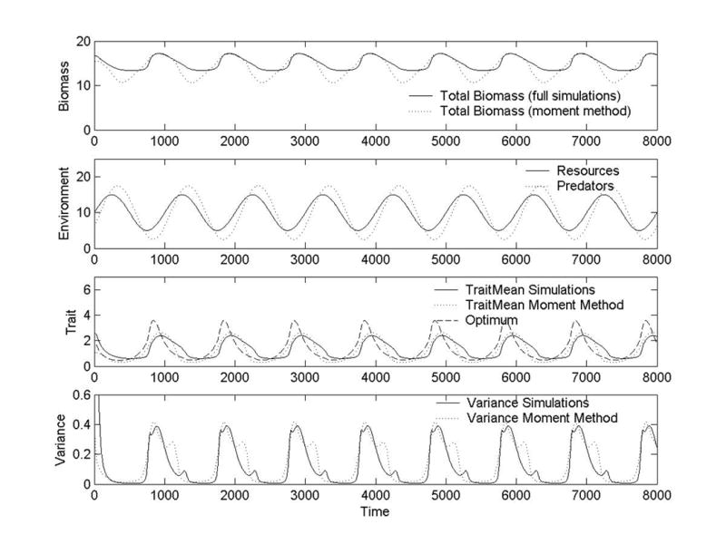
Plots of total biomass, environmental variables (resource abundance and predator population density), mean trait, optimal trait, and trait variance versus time based on simulations of both the exact equations (full simulations) and the moment-closure approximations. This simulation is for a frequency dependent growth function (Eq. (6)) using the parameter values d = 0.05, δ = 0.05, b = 1, μ = 1, h = 100. The environmental variables were chosen to be $E_1=10+5\sin \left(\frac{2\pi t}{1000}\right)$ and $E_2=10+7.5sin\left(\frac{2\pi t}{1000}+100\right)$. Total immigration per time step is 0.001.

To depict how well this system tracks the environment, we also plot the optimal trait– the trait value at which growth rate is maximum for the current environment (Panel 3, Fig. 1). The difference between this optimal trait and the mean trait for the community (also shown in Panel 3) reflects how well the system is tracking the fluctuating environment. As seen in Fig. 1, the response of the mean trait is delayed compared to the changes in the optimal trait and environment. This time delay is due to the finite time it takes for the community to change its composition, and results in fluctuations in the mean trait (community) being flatter than those in the optimal trait and environment. In Sec. (5) we directly relate the optimal trait to the environmental driver, making it even easier to interpret how well the ecosystem tracks the environment by using plots like those in Panel 3 of Fig. 1. Further, although the results are not shown here, decreasing the fluctuations in the environment (i.e., the amplitude and/or frequency of the environmental drivers) dampens the dynamics of the mean and variance, and the match between the moment-closure approximation and the full simulation improves.

There are two special cases of Eq. (5) that are also of potential biological interest. In Appendix 1, we explain these two cases and thus, how frequency dependence can be applied more broadly.

4 Functional complementarity

In communities with functional complementarity–a form of niche differentiation–ecosystem productivity increases through more efficient uptake of resources (Frost et al., 1995). Species have differential access to the pool of resources, and the total resources available to the community is larger than that available to any single species. A number of mechanisms underlying functional complementarity have been proposed, but its hallmark is over-yielding, corresponding to increased total productivity (i.e., higher rates of biomass production) when comparing the productivity for an assemblage of species to that of any single species in isolation (Tilman et al., 1997). One potential mechanism that gives a pattern consistent with functional complementarity is described in niche differentiation models with exploitative competition (Tilman and Lehman, 1997). Another potential mechanism is that facilitation (positive synergy) among species in a diverse community leads to increased efficiency of resource usptake and increased productivity (Bruno et al., 2003). Either of these mechanisms, exploitative competition or positive, synergistic interactions, have a strong frequency dependent component as well as a density dependent component.

To date, trait-based approaches have incorporated only a temporal sampling effect in explaining ecosystem function. The sampling effect (Loreau and Hector, 2001) postulates that the number of initial species increases the chance of a very efficient species being present and thus, increases the growth rate of the community once these species come to dominate through competitive exclusion. Within a fluctuating environment, which species has the maximal growth rate will continually change, increasing the likelihood that diverse communities will have higher rates of productivity than communities composed solely of the species with the highest productivity averaged over time (Norberg et al., 2001; Chesson et al., 2002). Distinguishing this temporal sampling effect from other effects, like functional complementarity, is difficult because both types of effects can lead to similar patterns of over-yielding. Despite the similar pattern, this over-yielding due to temporal sampling is distinct from that due to resource complementarity which can occur even within static environments and when a single species always has the maximal growth rate. Detailed treatments of complementarity that make the spatial structure explicit and heterogeneous can be used to model differential access to resources among different species/trait values, as discussed in Pacala and Levin (1997). For our purposes, we incorporate a simple form of frequency dependence that allows us to study functional complementarity and temporal sampling effects within the same model and to investigate their relative control over changes in rates of productivity in response to environmental change.

For any two trait values, z and z′, the strength of competition between organisms with these traits is described by an interaction function α(z, z′). We use this interaction function to construct a generalized form of the growth function in Eq. (1),

$$f(E,z)=h_1(E,z)\left(1-\frac{\int \alpha (z,z^{\prime })C(z^{\prime })d{z}^{\prime }}{K(z)}\right)+h_2(E,z).$$ (7)

The function h₁(E, z) represents the component of the growth function that is modulated by density-dependent effects, and for simple logistic growth it is equal to the the intrinsic rate of increase r. The component of the growth function that is not density dependent is represented by h₂(E, z) and can be used to model intrinsic mortality or constant rates of immigration.

Inserting Eq. (7) into Eq. (1) gives

$$\dot{C}(z)=\left(h_1(E,z)\left(1-\frac{\int \alpha (z,z^{\prime })C(z^{\prime })d{z}^{\prime }}{K(z)}\right)+h_2(E,z)\right)C(z)+i(z).$$ (8)

These equations are now able to account for the frequency dependent component of exploitative competition (α(z, z′) > 0) or positive, synergistic interactions (α(z, z′) < 0) and thus functional complementarity through α(z, z′). The density dependent component of functional complementarity is accounted for by K(z). When there is full complementarity and species experience no competition, α(z, z′) becomes a Dirac delta function δ(z − z′), so f(E, z) = h₁(E, z)(1 − C(z)/K(z)) + h₂(E, z). This reflects that each species population growth depends on just its own carrying capacity and is not affected by any other species.

We use this framework to study an example of competition and coexistence among plants. Our results demonstrate that complementarity in resource use not only leads to over-yielding (Tilman et al., 1996) but also plays a crucial role in maintaining trait variance. Two non-neutral mechanisms are often proposed to explain how plant species coexist: 1. phenological effects–species with different periodic timings for biological functions that are tied to climatic conditions, such as different nutrient uptake rates that depend on the season (e.g., R* theory (Tilman, 1982)), and 2. niche differentiation–resource competition among species being separated either in time or space, such as above/below ground competition for light and water/nutrients respectively (Fargione and Tilman, 2005). To model these effects, we define species in terms of trait values for nutrient uptake capability, z. To model niche differentiation, we use logisitic-growth type equations to describe how species compete for space and other resources to grow. Specifically, the carrying capacity, K(z), of each species can be interpreted as the maximum standing crop of that species in a monoculture with limitless nutrients. To induce phenological effects within temperate environments, we let the conversion of resources into biomass, p(t) = sin(t/365) + 1, and thus the growth rate, vary seasonally.

Combining this we have a growth function that describes the specific growth rate of a species with nutrient uptake ability, z, in an environment described by N_r for nutrients per area and p for the variation in growth rate due to seasonal variation in temperature, light, and other factors.

$$f(C(z),N_r,p,C_T,z)=p\left(1-\frac{\alpha C_T+(1-\alpha )C(z)}{K}\right)\left(\frac{N_r}{\frac{1}{z}+N_r}\right)-(m+\mathit{cz}).$$ (9)

In this equation m is mortality rate and c describes the metabolic cost of investing in a high trait value, z. The factor (1−α)C(z) forces the total intra-specific competition coefficient to always be 1 and usually differs from the level of inter-specific competition represented by α. These terms model competition for resources such as light, for which shading due to differing tree heights and structures (traits) plays a crucial role in determining differential access among different species/trait values (functional complementarity). The factor $\left(\frac{N_r}{\frac{1}{z}+N_r}\right)$ is a Monod Function that describes competition for a resource like nitrogen and dictates a maximum growth rate even when resource supply is limitless (Tilman, 1982; Wirtz and Eckhardt, 1996). (To explicitly relate this to our previous equations, h₁(p, z) = pN_r/((1/z) + N_r), h₂(z) = −(m + cz), K(z) = K, α(z, z) = α when z ≠ z (inter-specific competition), and α(z, z) = 1 when z = z (intra-specific competition).)

To illustrate the effects of different levels of functional complementarity, we perform simulations for two different values of α. We chose α = 1 to represent the absence of complementarity with equal intra-specific and inter-specific competition among all species. We also chose α = 0.5 to represent a greater degree of complementarity than for α = 1 and higher levels of competition among individuals of the same species than among individuals of different species. (Note that using the equations from Sec. (6), Eq. (9) can also be modeled as a two-trait system in which one trait is the strength of intra-specific competition and the other trait is the strength of inter-specific competition.)

For our simulations the nutrient dynamics are explicitly modeled by

$$\frac{d{N}_r}{\mathit{dt}}=\mathit{inp}-{\int }_0^{\infty }C(z)[f(C(z),N_r,p,C_T,z)+(m+\mathit{cz})]\mathit{dz}-N_{r}d$$ (10)

where d is the dilution rate in the soil, inp is the combined nutrient inputs of weathering, atmospheric load, and heterotrophic deposition, and the second term reflects the nutrient uptake rate of the plants. This assumes that the loss terms (m + cz) are not recycled, and for our simulations, we use a fixed input rate (rather than a dilution term as in Tilman 1982, Ch.3) to mimic weathering and atmospheric deposition.

Over-yielding is the amount of surplus production that exists in mixed cultures as compared to monocultures. To measure over-yielding, we thus calculate the biomass yield for our simulated systems relative to either the maximum yield of any species in monoculture or the weighted average of the species yields in monocultures (e.g. Loreau and Hector 2001, Beckage and Gross 2006). Choosing lower values of α, corresponding to higher levels of complementarity, immediately leads to faster rates of biomass production, i.e., over-yielding, and to larger total biomass. Ignoring the term (1 − α)C(z) in Eq. (9), which is often negligible, the carrying capacity, K, can be rescaled to include the factor α as K_new ≈ K/α, so that lower values of α can be interpreted as larger values for the carrying capacity, leading to faster rates of productivity, i.e., over-yielding, and larger total biomasses. In particular, the approximate ratio of biomass for a system with complementarity, α, to the biomass of a monoculture is K_new/K ≈ 1/α, showing that maximum total biomass is inversely proportional to α. This effect of complementarity is biologically realistic and important but is a mathematically trivial consequence of our framework.

To reveal the qualitative dependence of the system dynamics on the value of α, we can normalize for the straightforward effect of complementarity on over-yielding by scaling the carrying capacity as K → αK. As discussed above, this scaling neglects a factor of (1 − α)C(z) that is usually negligible, and indeed, as seen in panel 3 of Fig. 2, the biomass difference between the scaled simulation with α = 0.5 ; K∗ = 5 and the baseline simulation α = 1; K∗ = 10 is very small. Using this scaling makes the total biomass nearly equivalent for systems with different values of α, and allows us to demonstrate that complementarity leads to reduced competition and higher trait diversity, independent of the effects of over-yielding. We perform simulation and present figures with both the un-normalized and normalized versions of the carrying capacity, K, to display the separate effects of over-yielding and larger trait diversity.

Figure 2.

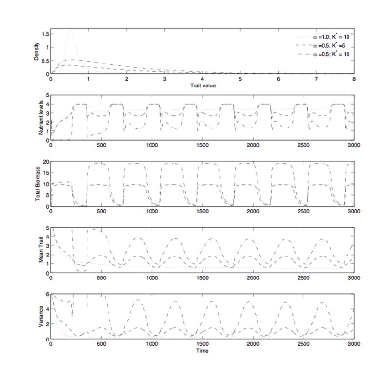
Simulation results for Eqs. (9-10) using the parameter values p = 1, m = 0.01, c = 0.02, inp = 0.2, d = 0.1, and a total immigration per time step of 0.001. The results are for three different simulations corresponding to α = 1 with a carrying capacity of K^* = 10 and to α = 0.5 with carrying capacities of K^* = 5 and K^* = 10. We use the notation K^* here, instead of K as in Sec. (4), to differentiate between the un-normalized (K) and normalized (K → αK) carrying capacities. For α = 1, K = αK, so K^* = 10 represents both cases. For α = 0.5, K^* = 10 is the un-normalized carrying capacity and K^* = α10 = 5 is the normalized value. The simulation with α set to 1 represents high competition/low complementarity and 0.5 represents low competition/high complementarity. For α = 0.5 the un-normalized value of the carrying capacity (K^* = 10) corresponds to over-yielding and larger total biomass (maximal biomass of 20), while the normalized value (K^* = 5) accounts for the effects of over-yielding and total biomass (maximal biomass of 10), revealing the effects of complementarity that are due solely to reduced competition. Panel 1 displays the trait distribution density as a function of the trait z, where values were averaged over the last cycle of the simulation. Panel 2 shows the dynamics of nutrients mainly as determined by seasonal changes in productivity. Panel 3 shows the total community biomass, C_T . Panel 4 depicts the mean trait for each community. Panel 5 displays the dynamics of the trait variance and shows that increased complementarity in resource use leads to greater trait variance.

The results of our numerical simulations for α = 0.5 and α = 1 are presented in Fig. 2. This figure demonstrates that the value of α, and thus the form of the interaction and growth functions, impact the dynamics and biomass of the system. In Panel 1 of Fig. 2, we see that complementarity (α = 0.5) results in a wider distribution (larger trait variance) and a larger trait mean (1.877 compared to 1.164) regardless of whether the carrying capacity, K, has been normalized or not. Also, the evenness index for this community is larger when complementarity is higher, 0.342 for α = 0.5 as compared with 0.317 for the community with α = 1. Further, Panel 2 displays that complementarity results in greater total nutrient uptake by the community and, therefore, lower nutrient levels. These effects occur independent of the normalization of K but are much more pronounced when over-yielding, corresponding to an un-normalized K, is present because total biomass is much larger (see Panel 3). After our approximate normalization for the effects of complementarity on total biomass, (K → αK), higher complementarity actually results in lower total biomass than in the absence of complementarity (α = 1) (as seen in Panel 3). This reduced biomass is because the trait distribution is more skewed towards species with high z, corresponding to better nutrient uptake but also higher overall metabolic costs, cz. In the community with higher complementarity (α = 0.5), the dynamics of the mean trait are always affected more by seasonal changes in productivity than in the community with full competition (α = 1) (see Panel 4). Finally, from the dynamics of the trait variance displayed in Panel 5, we observe that increased complementarity maintains trait variance throughout the simulation and not just during the last cycle (as shown in Panel 1). With complementarity (α = 0.5), the mean and variance are higher for the un-normalized (over-yielding) case due to the associated, larger fluctuations in total biomass and nutrient levels.

In classic R* theory, all species have equal access to all resources, and all competition among species is mediated by how quickly each species consumes the resources, thus removing it from the pool that is available to the other species (Tilman 1982). This is in distinct contrast to complementarity, and thus, there are no factors, like ones in our framework, to account for the effects of complementarity. Indeed, Pacala and Levin (1997) go a step further and provide a more mechanistic explanation for resource supply, uptake, and complementarity in which spatial heterogeneity dictates differential access to resources among different species.

To relate our framework to R* theory, we consider a monoculture of species, z, (i.e., C(z′) = C_T for z′ = z and is zero otherwise), leading to a simplified form of Eq. (9). Then, by setting f = 0 we solve for the minimum amount of resources required for non-negative growth

$$N_r^{\ast }=\frac{1}{z}\frac{1}{\left[\frac{p(1-\frac{C_T}{K})}{(m+\mathit{cz})}-1\right]}$$ (11)

Species with negative values for $N_r^{\ast }$ are not viable because loss rates are greater than growth rates, just as for the analogous equation from Tilman (1982, Eq. (6) on p. 97).

Within R* theory $N_r^{\ast }$ determines the competitive ability of species because species that can grow at lower values of resources, as dictated by $N_r^{\ast }$, will be able to continue growing while other species are pushed to extinction. This results in the species with the lowest values of $N_r^{\ast }$ displacing (competitively excluding) all other species (Tilman 1982). By contrast, the optimal trait, meaning the trait with the highest rate of growth, is given by

$$z_{\mathit{opt}}=-\frac{1}{N_r}+\sqrt{\frac{p(1-\frac{C_T}{K})}{c{N}_r}}$$ (12)

For the example modeled using our framework, when competition is high (α = 1) and nutrients are abundant, the simulations suggest that species that initially grow most quickly and establish a large biomass will outcompete species that are more specialized for nutrient uptake but grow more slowly. For communities of this type, turn-over rates will be low (the term $\left(1-\frac{\alpha C_T+(1-\alpha C(z))}{K}\right)\left(\frac{N_r}{(1/z+N_r)}\right)$ becomes small) and as nutrients drop during peak season, the nutrient-uptake specialized species are unable to outcompete the early, quickly growing species. This phenomena is not present when complementarity is strong (α = 0.5) because the nutrient-uptake specialized species can gain biomass, and thus establish some foothold, at the beginning of the growth period, despite the physiological advantage of the quickly growing species.

Our simulations for these systems, as seen in Fig. 2 also reveal that higher complementarity results in faster exploitation of the nutrients and hence a reduction in nutrient concentrations during peak growth season. Since nutrient loss from the system is proportional to nutrient concentration, this suggests nutrient leakage is lower with higher complementarity. This result has relevance to ecosystem services, conservation, and management because biodiversity conservation may prevent nutrient leakage.

Biological systems have the potential to give rise to many other forms for α(z, z′). These equations can be naturally divided into three cases: 1) α(z, z′) are equal for all species pairs, i.e., all pairings of z and z′, so that α(z, z′) = α. 2) The interaction function, α(z, z′) correlates with trait, z, or follows some distribution in z, so that α(z, z′) = α(z). and 3) α(z, z′) are species-pair specific. Our growth function Eq. (9) falls into case (1) for α = 1 and case (3) for α = 0.5. Interestingly, cases (1) and (2) reduce to the same form, and for a certain class of examples, case (3) also reduces to this same form. We discuss these similarities in Appendix 2 to demonstrate the range of systems that might be explored using our framework. The methods for solving these cases are the same as described above and can be simulated using moment-closure approximations as in Norberg et al. (2001).

5 Relating the optimal trait to the environmental variable

Within a fixed environment, there is a set of traits for which population growth is maximal, and this defines the optimal traits for that environment. As environments fluctuate, the optimal traits will change, and the differences between the optimal traits and the mean traits, which characterize the current state of the community, indicate how well the community is adapting to environmental change. To develop a useful diagnostic for measuring the ability of ecosystems to respond to environmental change, we directly relate optimal traits to their corresponding environmental variables. This relation eases the interpretation and enhances the intuition for how the community tracks and adapts to the environment.

Often, there is a single trait that is optimal for a specific environment. As seen in our model of functional complementarity and sampling effects, relating the optimal trait to the environment can help with interpretation of mechanisms underlying ecosystem response to environmental change (particularly in the context of productivity). To begin, we consider systems where each trait is affected by a single environmental variable. Given a growth function with a single trait, f(E,C_T , z), we find the optimal trait, z_opt, by solving

$$\frac{\partial f(E,C_T,z)}{\partial z}=0$$ (13)

When there is only one solution, g(E,C_T), that satisfies, $\frac{{\partial }^{2}f(E,C_T,g(E,C_T))}{\partial z^2}<0$, then there is a unique optimal trait given by z_opt = g(E,C_T). We then let

$$z=g(Z,C_T),$$ (14)

and let Z vary such that z has the same range as before. Consequently, Z can be considered the new definition of the trait, and since z_opt occurs at Z_opt, by Eq. (14) we have z_opt = g(Z_opt,C_T) = g(E,C_T) and therefore,

$$Z_{\mathit{opt}}=E.$$ (15)

Here, the growth function is analogous to a fitness function in quantitative genetics with a single attractive peak such that under selection the average trait moves towards the optimum.

When there are multiple traits and environmental variables, the equation for the optimal trait becomes

$$\sum _{\eta =0}^N\frac{\partial f(\overrightarrow{E},C_T,\overrightarrow{z})}{\partial z_{\eta }}=0,$$ (16)

where $\overrightarrow{E}=(E_1,E_2,\dots ,E_J)$ and $\overrightarrow{z}=(z_1,z_2,\dots ,z_N)$. If $\frac{\partial f(\overrightarrow{E},C_T,\overrightarrow{z})}{\partial z_{\eta }}=0$ for each η and each trait is associated with a single environmental variable so that J = N, then Eqs. (13-15) can be used separately for each z_η. In that case ${\overrightarrow{z}}_{\mathit{opt}}=(z_{1,\mathit{opt}},z_{2,\mathit{opt}},\dots ,z_{N,\mathit{opt}})$. When Eq. (16) cannot be separated in this way, a Jacobian must be used to simultaneously choose the correct redefinitions of all traits. In fact, when there are multiple optima that all lie along a line, e.g., z_1,opt = z_2,opt, it is often possible to choose a new and entirely different set of traits that are each a function of all of the original traits, e.g., Z₁ = u₁(z₁, z₂) and Z₂ = u₂(z₁, z₂).

For the redefinition in Eq. (14) to apply globally, g(E,C_T) must be one-to-one. When there are multiple optima, i.e., multiple solutions to Eq. (13), it is not possible to find a one-to-one mapping because g(E,C_T) must necessarily equal multiple z_opt. However, local analyses can still be performed by using Eqs. (14-15) at each optima.

Given any set of arbitrary growth functions, each with a single optima, we can use the procedure above. However, three other scenarios are more problematic. First, in practice it may not be possible to solve the equation $\frac{\partial f(E,C_T,z)}{\partial z}=0$ for z_opt = g(E,C_T), in which case we cannot write down a simple equation for Z as z = g(Z,C_T). Second, different traits may depend on the same environmental variable, E. For example, reproductive times and lifespans may both depend on temperature. Although the traits share the same environmental variable, their dependence on E can still be treated separately, and each trait can be redefined to have an optima at E with no new difficulties. Correlations between these traits may make it impossible to track E, but that does not prevent these redefinitions, which contain no information about the dynamics and whether or not the realized trait can converge to the optimal trait. Third, a single trait may depend on multiple environmental variables. In this case, the procedure above does not work, and one must either choose a single environmental variable relative to which other quantities are defined, or one can simply use the original equations.

6 Multiple, correlated traits and environmental drivers

In real ecosystems, response to environmental change is determined by the combined effects of multiple traits and multiple environmental drivers. How traits and drivers interact with one another constrains and alters the possible responses of ecosystems to environmental change. Here, we develop a multi-trait, multi-environmental driver version of trait-based frameworks to investigate how these interactions affect ecosystem response. We begin by deriving the equations for two traits and two environmental variables and use this to investigate how correlations between two traits affect the rate of response and growth of communities within fluctuating environments. We then generalize to N traits and drivers (details are in Appendix 3) because recent empirical work suggests that multiple traits are important (Reich et al., 2004; Shipley et al. 2006).

6.1 Two-trait system

For two traits Eq. (1) becomes

$$\dot{C}(z_1,z_2)=f(E_1,E_2,C_T,z_1,z_2)C(z_1,z_2)+i(z_1,z_2),$$ (17)

where C(z₁, z₂) is the biomass of guilds characterized by the two traits z₁ and z₂ and i(z₁, z₂) is a term that accounts for migration. We consider the traits to be continuous and C, f, and i to be continuous functions of these variables. E₁ and E₂ account for environmental effects on the biomass, and C_T is the total biomass, which is given by ${\int }_{z_2,z_1}C(z_1,z_2)\hspace{0.17em}d{z}_{1}d{z}_2$. Proceeding as in Sec. (2), we Taylor expand f to find

$${\dot{C}}_T=C_T\sum _{i=0}^{\infty }\sum _{j=0}^{\infty }{f}^{(i,j)}(E_1,E_2,C_T,{\overline{z}}_1,{\overline{z}}_2)M_{i,j}+I.$$ (18)

The average values of the traits, ${\overline{z}}_1$ and ${\overline{z}}_2$, are given by

$${\overline{z}}_1=\frac{1}{C_T}{\int }_{z_2,z_1}{z}_{1}C(z_1,z_2)d{z}_1\hspace{0.17em}d{z}_2;\hspace{0.17em}\mathrm{\hspace{0.17em} }{\overline{z}}_2=\frac{1}{C_T}{\int }_{z_2,z_1}{z}_{2}C(z_1,z_2)\hspace{0.17em}d{z}_1\hspace{0.17em}d{z}_2.$$ (19)

I is the total immigration across all traits,

$$I={\int }_{z_2,z_1}i(z_1,z_2)\hspace{0.17em}d{z}_1\hspace{0.17em}d{z}_2.$$ (20)

M_i,j are the central moments,

$$M_{i,j}=\frac{1}{C_T}{\int }_{z_2,z_1}C(z_1,z_2){(z_1-{\overline{z}}_1)}^i{(z_2-{\overline{z}}_2)}^j\hspace{0.17em}d{z}_1\hspace{0.17em}d{z}_2,$$ (21)

and the explicit form of the Taylor series expansion for f is

$$f(E_1,E_2,C_T,z_1,z_2)=\sum _{i=0}^{\infty }\sum _{j=0}^{\infty }{f}^{(i,j)}(E_1,E_2,C_T,{\overline{z}}_1,{\overline{z}}_2){(z_1-{\overline{z}}_1)}^i{(z_2-{\overline{z}}_2)}^j,$$ (22)

where

$$f^{(i,j)}(E_1,E_2,C_T,{\overline{z}}_1,{\overline{z}}_2)=\frac{1}{i!j!}[{\partial }_{z_1}^i{\partial }_{z_2}^{j}f(E_1,E_2,C_T,z_1,z_2)]{\mid }_{z_1={\overline{z}}_1,z_2={\overline{z}}_2}.$$ (23)

To derive the equations for the rate of change of the average traits, we define $S_{z_1}={\overline{z}}_1{C}_T$ and take its time derivative to obtain

$${\dot{S}}_{z_1}=C_T\sum _{i=0}^{\infty }\sum _{j=0}^{\infty }{f}^{(i,j)}(E_1,E_2,C_T,{\overline{z}}_1,{\overline{z}}_2)[M_{i+1,j}+{\overline{z}}_1{M}_{ij}]+I{\stackrel{\sim }{z}}_1,$$ (24)

where

$${\stackrel{\sim }{z}}_1=\frac{{\int }_{z_2,z_1}{z}_{1}i(z_1,z_2)\hspace{0.17em}d{z}_1\hspace{0.17em}d{z}_2}{I}.$$ (25)

Using this, we can show

$${\dot{\overline{z}}}_1=\sum _{i=0}^{\infty }\sum _{j=0}^{\infty }{f}^{(i,j)}(E_1,E_2,C_T,{\overline{z}}_1,{\overline{z}}_2)M_{i+1,j}+\frac{I}{C_T}({\stackrel{\sim }{z}}_1-{\overline{z}}_1).$$ (26)

In exact analogue, or by realizing the equations are symmetric under z₁ → z₂ along with i→ j, we also find

$${\dot{\overline{z}}}_2=\sum _{i=0}^{\infty }\sum _{j=0}^{\infty }{f}^{(i,j)}(E_1,E_2,C_T,{\overline{z}}_1,{\overline{z}}_2)M_{i,\mathrm{j}+1}+\frac{I}{C_T}({\stackrel{\sim }{z}}_2-{\overline{z}}_2).$$ (27)

Generalizing this method to derive equations for the rate of change of all the central moments, we define S_i,j = C_TM_i,j and find

$$\begin{array}{c}{\dot{S}}_{i,j}=C_T\sum _{l=0}^{\infty }\sum _{m=0}^{\infty }{f}^{(l,m)}(E_1,E_2,C_T,{\overline{z}}_1,{\overline{z}}_2)[M_{i+l,j+m}-i{M}_{l+1,m}{M}_{i-1,j}-j{M}_{l,m+1}{M}_{i,j-1}]\\ +I{M}_{i,j}^w-iI({\stackrel{\sim }{z}}_1-{\overline{z}}_1)M_{i-1,j}-jI({\stackrel{\sim }{z}}_2-{\overline{z}}_2)M_{i,j-1},\end{array}$$ (28)

where

$$M_{i,j}^w=\frac{1}{I}{\int }_{z_2,z_1}{(z_1-{\overline{z}}_1)}^i{(z_2-{\overline{z}}_2)}^{j}i(z_1,z_2)\hspace{0.17em}d{z}_1\hspace{0.17em}d{z}_2=\sum _{l=0}^i\sum _{m=0}^j\left(\begin{array}{c}i\\ l\end{array}\right)\left(\begin{array}{c}j\\ m\end{array}\right){({\stackrel{\sim }{z}}_1-{\overline{z}}_1)}^{i-l}{({\stackrel{\sim }{z}}_2-{\overline{z}}_2)}^{j-m}{\stackrel{\sim }{M}}_{l,m},$$ (29)

and

$${\stackrel{\sim }{M}}_{l,m}=\frac{1}{I}{\int }_{z_2,z_1}{(z_1-{\stackrel{\sim }{z}}_1)}^l{(z_2-{\stackrel{\sim }{z}}_2)}^{m}i(z_1,z_2)\hspace{0.17em}d{z}_1\hspace{0.17em}d{z}_2.$$ (30)

From the above, we obtain

$$\begin{array}{c}{\dot{M}}_{i,j}=\sum _{l=0}^{\infty }\sum _{m=0}^{\infty }\\ f^{(l,m)}(E_1,E_2,C_T,{\overline{z}}_1,{\overline{z}}_2)\\ \times [M_{i+l,j+m}-i{M}_{l+1,m}{M}_{i-1,j}-j{M}_{l,m+1}{M}_{i,j-1}-M_{l,m}{M}_{i,j}]\\ +\frac{I}{C_T}[\sum _{l=0}^i\sum _{m=0}^j\left(\begin{array}{c}i\\ l\end{array}\right)\left(\begin{array}{c}j\\ m\end{array}\right){({\stackrel{\sim }{z}}_1-{\overline{z}}_1)}^{i-l}{({\stackrel{\sim }{z}}_2-{\overline{z}}_2)}^{j-m}{\stackrel{\sim }{M}}_{l,m}\\ -i({\stackrel{\sim }{z}}_1-{\overline{z}}_1)M_{i-1,j}-j({\stackrel{\sim }{z}}_2-{\overline{z}}_2)M_{i,j-1}-M_{i,j}].\end{array}$$ (31)

These equations completely define the two-trait problem.

6.2 Effects of correlations among traits and drivers on the dynamics of ecosystem response

We investigate how trait and driver correlations affect ecosystem response in the context of a predator-prey system within a temperate habitat. Our growth function for the system is

$$f(E_1,E_2,C_T,z_1,z_2)=p\left(1-\frac{{(E_1-z_1)}^2}{{\sigma }^2}\right)\left(1-\frac{C_T}{K}\right)-r{z}_2-e^{-z_2}g{E}_2-d$$ (32)

where z₁ is a trait that represents the temperature at which growth rate is maximum for organisms with that trait, E₁ is the environmental temperature, and σ determines how quickly growth rate declines as the distance between the optimal temperature for growth, z₁, for a given organism and the environmental temperature increases (Norberg et al., 2001). For the predator-prey parts of the growth function, p is the per capita fertility of the species in the absence of density effects, K is carrying capacity, g is per capita feeding rate, E₂ is the ratio of the number of predators to the number of prey, and z₂ is a trait that represents investment in predator defense.

In Fig. 3 we depict the biomass for growth functions for each trait separately (Eq. (32) with z₂ = E₂ = 0 (optimal temperature) and z₁ = E₁ = 0 (predator-prey dynamics)) as well as the two traits combined, Eq. (32). Although the dynamics of the biomass for the two-trait system are similar to those for the single-trait system for z₁ as seen in the figure, the dynamics of the biomass for the two-trait system are not just a superposition of the two single-trait systems. In Fig. 4 we compare the mean trait values and trait variances as computed from the single- and two-trait simulations, and we show the covariance between the two traits grows to appreciable levels at many times during the simulation. This nonzero covariance, which results from immigration and environmental correlations as described below, leads to intriguing dynamics with potentially significant ecological implications.

Figure 3.

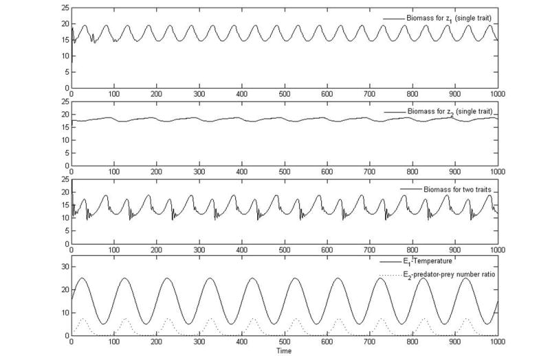
Plots of biomass versus time for growth functions modeling tradeoffs in optimal temperature (panel 1), predator-prey dynamics (panel 2), and the combined effects of predator prey and optimal temperature (panel 3), as well as a plot (panel 4) of the environmental variables (temperature and predator density) versus time. All of these use Eq. (32). For optimal temperature alone, the parameter values are p = 5,σ² = 2, K = 20, d = 0.1, $E_1=15+10sin\left(\frac{2\pi t}{100}\right)$, r = 0, g = 0, E₂ = 0, and z₁ = 0. For predator-prey dynamics alone, the parameter values are p = 5, K = 20, r = 0.1, g = 1, d = 0.1, $E_2=2sin\left(\frac{2\pi t}{100}+25\right)$, E₁ = 0, and z₂ = 0. For combined effects of predator-prey dynamics and optimal temperature tradeoffs, the parameter values are p = 5, σ² = 2, K = 20, d = 0.1, $E_1=15+10sin\left(\frac{2\pi t}{100}\right)$, r = 0.1, g = 1, and $E_2=2sin\left(\frac{2\pi t}{100}+25\right)$. Total immigration per time step is 0.1 for the single-trait simulations and 1 for the two-trait simulations. More immigration is necessary for the two-trait case because there are many more functional groups (species), and immigration occurs for each one.

Figure 4.

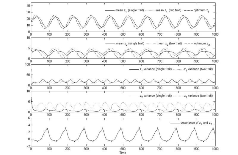
Plots of trait mean for optimal temperature, z₁ (panel 1), investment in predator defense, z₂ (panel 2), variance in z₁ (panel 3) and z₂ (panel 4), and covariance between z₁ and z₂ (panel 5) versus time for growth functions modeling tradeoffs in predator-prey dynamics, optimal temperature, and the combined effects of predator prey and optimal temperature. These are results from the same simulations as in Fig. (3). The simulations all use Eq. (32). For optimal temperature alone, the parameter values are p = 5, σ² = 2, K = 20, d = 0.1, $E_1=15+10sin\left(\frac{2\pi t}{100}\right)$, r = 0, g = 0, and E₂ = 0. For predator-prey dynamics alone, the parameter values are p = 5, K = 20, r = 0.1, g = 1, d = 0.1, $E_2=2sin(\frac{2\pi t}{100}+25)$, E₁ = 0, and z₂ = 0. For combined effects of predator-prey dynamics and optimal temperature tradeoffs, the parameter values are p = 5, σ² = 2, K = 20, d = 0.1, $E_1=15+10sin\left(\frac{2\pi t}{100}\right)$, r = 0.1, g = 1, and $E_2=2sin\left(\frac{2\pi t}{100}+25\right)$. Total immigration per time step is 0.1 for the single trait simulations and 1 for the two-trait simulations. More immigration is necessary for the two-trait case because there are many more functional groups (species), and immigration occurs for each one.

For example, this correlation significantly changes the trait means and variances as seen by comparing the results of the two-trait simulations to those for the single traits. The trait variances are higher when the traits are modeled together (the two-trait simulation) because the covariance causes each trait to be pulled further away from its respective mean. This increased variance allows z₂ to track the optimal trait better in the two-trait, than in the one-trait, simulation. This results shows that inducing correlations between traits can actually allow populations to more successfully adapt to their environments and counters the naive expectation that populations will best adapt to the environment when only a single trait is being optimized, i.e, is subject to selection pressures and sorting processes. This naive argument is incorrect because it ignores the importance of the trait variance. A large trait variance leads to greater diversity in the population by maintaining small numbers of organisms with traits far from the optimum. These small numbers can grow rapidly, and thus the population can respond rapidly to quick changes in the environment. This intriguing result reveals a crucial role for biodiversity in controlling and improving ecosystem response to environmental change.

It should also be noted, however, that the higher variance in trait diversity created by these correlations leads to the presence of less efficient functional groups, as compared to the uncorrelated case, and thus lowers the total biomass of the community. Since the amount of total biomass can impact the stability and persistence of ecosystems, the benefit of being able to better track the environment and optimal traits, as discussed above, must be weighed against the detriment of this decrease in total biomass. As seen in Fig. 3, correlations only slightly lower the total biomass for our example, and that is because of the low abundance of organisms with traits that are far from the optimum. Although these rare organisms have a small yet noticeable effect on the total biomass, they nevertheless increase the trait diversity enough to affect the communities ability to track the environment.

Several general conclusions about the existence and effects of correlations in ecosystem dynamics follow from our two-trait equations (Eq. (31)). Correlations–defined by M_i,j ≠ 0 for both i and j greater than zero–are absent when: (i) z₁ and z₂ are uncorrelated and (ii). C(z₁, z₂) is separable. In this case, M_1,1 becomes the product of M_1,0 and M_0,1, both of which are zero. We have thus identified two conditions, corresponding to mechanisms, by which correlations arise. The first mechanism violates (i), so that a change in one trait causes a change in another trait. This corresponds to the most obvious type of correlation and can occur due to genetic correlations or developmental coupling, e.g, cell size and cell number. The second mechanism violates (ii), so that, for example, a single environmental variable simultaneously acts on or selects for both traits. This is reflected in the growth function, which will contain the linkage due to this type of selection and will affect whether C(z₁, z₂) is separable. Typically, C(z₁, z₂) will not be separable, indicating that correlations are present.

Furthermore, even when the traits are initially uncoupled and C(z₁, z₂) is separable, only special forms of immigration allow the equations to remain uncoupled as the system progresses in time. This effect can be seen by using i = j = 1 in Eq. (31) with all covariance terms equal to zero (M_i,j = 0 for both i and j greater than 0) and noting that the first central moments are zero at all times (M_1,0 = M_0,1 = 0), to obtain ${\dot{M}}_{1,1}~\frac{1}{C_T}[({\stackrel{\sim }{z}}_1-{\overline{z}}_1)({\stackrel{\sim }{z}}_2-{\overline{z}}_2)+({\stackrel{\sim }{z}}_1-{\overline{z}}_1){\stackrel{\sim }{M}}_{0,1}+({\stackrel{\sim }{z}}_2-{\overline{z}}_2){\stackrel{\sim }{M}}_{1,0}]$. Since immigration is often independent of the environmental factors that determine the average traits, the right side of this equation will almost certainly be nonzero. Thus, immigration induces a correlation, and as seen in Fig. (4), M_1,1 gains a nonzero part at each time step when performing simulations using discretized versions of the equations. Similar analyses hold for multi-trait and multi-driver systems using Eq. (46).

In many ecosystems, more than two traits and drivers will likely be needed to obtain biologically meaningful results, so in Appendix 3 we generalize this framework to the N-trait problem.

7 Discussion and Conclusions

Trait-based approaches are an intriguing and useful way to model the effects of a changing environment on natural selection and species sorting processes, biodiversity, and ecosystem dynamics. These approaches are being incorporated into empirical work, and hence, the development of related theoretical approaches is greatly needed (Tilman, 2001; Reich et al., 2003b & 2004; McGill et al., 2006; Shipley et al., 2006).

We applied and extended our trait-based approach to two ecological questions regarding how interactions affect ecosystem response to environmental change. In Sec. (4), by incorporating the interaction function, α(z, z′), into the the growth function, it becomes possible to simultaneously model and disentangle the temporal sampling effect and functional complementarity. This work constitutes an extension of R* theory, particularly with regard to dynamics and the role of sustaining trait variability. Moreover, in our example (Fig. 2), we show that increased complementarity helps maintain trait variance and reduce nutrient leakage. This has important consequences for ecosystem maintenance and for understanding the effects of biodiversity loss on habitats and on human resources.

On a global scale, climatic constraints, e.g., water availability, light, and temperature, vary across regions as well as over time (Nemani et al., 2003) and are often highly correlated. If traits that mitigate the effects of these climatic constraints are also correlated, the effects of climate change may be difficult to predict using current approaches (IPCC Report, 2001). In this paper, we showed that two correlated traits (optimal temperature for growth and predator-prey defense) can better maintain biomass and biodiversity than a system with uncorrelated traits. When correlations are present, each trait tracks the environmental conditions better than the system without correlations. This improved tracking is because the correlation induces a larger trait variance, leading to the survival of organisms with trait values that are less favorable in the current environment but may be well suited for new environments that arise. This illustrates not only that correlations among traits have quantitative effects on ecosystem dynamics, but that even the qualitative effects and behaviors are difficult to predict using intuition alone. This is exactly why analytical, quantitative frameworks, such as the one developed here, are crucially needed to help predict the complicated effects of climate change on biological systems and ecosystem dynamics. Indeed, there is great interest in investigating correlations between traits in terrestrial plants (Grime et al., 1997; Grime, 2003; Lavorel and Garnier, 2003) as well as in aquatic algae (Andersen, 1997; Reynolds, 1997) to predict species distributions and community response to environmental change (McGill et al., 2006).

To date, most trait-based models have been used to analyze the response of a single trait to changes in a single environmental variable. Reich et al. (2003b) has demonstrated that for grassland and savanna species of plants, functional groupings based on only a few, a priori traits, including nitrogen-fixing capacity, are often insufficient for determining responses to varying levels of nitrogen. Instead their work suggests that a suite of traits is necessary to model ecosystem response to environmental change. Moreover, Reich et al. (2004) showed that the response of biomass accumulation in plants to levels of carbon dioxide and nitrogen is affected both by species diversity and functional group diversity. Perhaps these independent effects are due to the coarseness of the functional groupings. If so, a trait-based model that incorporates a suite of traits will be an improvement over either species groupings or traditional functional groupings used alone. Irrespective of this, these studies provide evidence that models of ecosystem responses that are based on only a single or few traits are likely to be limited in their predictive capacity.

Several recent models have begun to address the effects of multiple environmental variables upon multiple traits. In particular, Chesson et al. (2002) studied the effects of light, nitrogen, and water availability upon community biomass. Loreau et al. (2003) extended this type of approach by explicitly including the effects of dispersal. Furthermore, Tilman (2004) analyzed the combined effects of temperature and a limiting resource, while simultaneously incorporating stochastic processes related to mortality. These studies represent significant progress toward understanding ecosystem dynamics and yield informative results. However, all of them focus on limiting resources, and none explicitly consider correlations among environmental variables or among species traits. These assumptions are often not valid. For example, when grasslands experience periods of drought, intense grazing, or extreme temperatures, factors besides resource uptake may be more important in shaping the community, even though resource retention is still determined by the plants resource uptake abilities (Tilman and Downing 1994).

For such systems, it is crucial to understand how traits are correlated to one another when compared across species. In the case that a correlation exists between nutrient uptake ability and grazing resistance, the ability of the community as a whole to use nutrients for biomass production would be affected by grazing pressure. Consequently, we have developed a general trait-based framework that explicitly models multiple, correlated traits and environmental drivers. Indeed, even though trait-based approaches by Chesson et al. (2002), Loreau et al. (2003), and Tilman (2004) differ from that of Norberg et al. (2001), our equations apply equally well to those frameworks so long as the correct correspondences between variables and functions are carefully identified.

Previous ecological work has provided many insights into the correlation between physiological aspects of species within certain groups (Grime et al. 1997; Reynolds, 1997). Our framework can be used to elucidate how time-varying, limiting factors, such as light, nutrients, drought or grazing affect the types of communities and even the diversity within these communities. Our framework allows these questions to be addressed in specific systems where a suite of correlated traits are important, as well as in a more general, theoretical context such as the examples presented in this paper. The next step is to perform numerical simulations for specific systems and to evaluate the accuracy of different types of moment-closure methods. After validation, we can apply this framework to empirical systems and simplify the equations involved. These are non-trivial next steps and will take considerable work to accomplish, but our preliminary results suggest it is feasible. By gaining a deeper understanding of how the environment impacts ecosystem dynamics and composition, it may be possible to predict and quantify many of the effects that scientists are beginning to discover (Visser et al., 1998; Visser and Holleman, 2001; Root et al., 2003), including the effects of global warming on ecosystem processes such as productivity (Finney et al. 2002) and the timing of events such as the budding of flowers (Parmesan and Yohe, 2003).

Appendix 1: Two special cases of frequency dependence

Here we show how two of the most common and simple forms of frequency dependence can be incorporated into our framework. First, we consider the case where every organism’s growth depends on the frequency of organisms with a single, specific trait value, z′. In this case, F(z, z′) = δ(z − z′), D(z) a Dirac delta function, so that D(z) = C(z′)/C_T and $\frac{\partial D(z)}{\partial z}=(1/C_T)(\partial C(z^{\prime })/\partial z)=0$. Thus, the extra terms in Eq. (5) that arise rom the chain rule applied to D(z) are zero, and the mathematical structure of Eqs. (2-3) are identical to those of Norberg et al. (2001). However, because the dependencies of the growth function change, the effects of frequency dependence on the dynamics of the quations could still exhibit novel qualitative behavior and provide informative results.

Second, we consider the case where the growth rate of organisms with trait z depends on the relative frequency compared with that of organisms with the mean trait, $\overline{z}$. As a simple example, we choose $F(z,z^{\prime })=F(z,\overline{z})=\delta (z)-\delta (\overline{z})$ when $C(z)>C(\overline{z})$ and $F(z,z^{\prime })=F(z,\overline{z})=\delta (\overline{z})-\delta (z)$ when $C(\overline{z})>C(z)$. This results in $D(z)=\mid C(z)-C(\overline{z})\mid /C_T$, and thus, $\frac{\partial D(z)}{\partial z}=(1/C_T)(\partial C(z)/\partial z)$ when $C(z)>C(\overline{z})$ and $\frac{\partial D(z)}{\partial z}=-(1/C_T)(\partial C(z)/\partial z)$ when $C(\overline{z})>C(z)$. That is, the growth function is modulated according to the slope of the biomass distribution. These frequency-dependent distributions result in different dynamics than in Norberg et al. (2001), and they are described by the modified equations given in Eq. (5).

Appendix 2: General forms of functional complementarity

Here we show how to incorporate certain types of functional complementarity into our trait-based equations. Recall that in Sec. (4) we separated complementarity into three cases, and the first two cases were: 1) α(z, z′) are equal for all species pairs, i.e., all pairings of z and z′, so that α(z, z′) = α. and 2) The interaction function, α(z, z′) correlates with trait, z, or follows some distribution in z, so that α(z, z′) = α(z).

Showing the equivalence of cases (1) and (2) is straightforward. Multiplying Eq. (8) by α(z), using the fact that α(z) is independent of time so that d/dt does not act on it, and defining the new variables, Y (z) = α(z)C(z) and L(z) = α(z)i(z), it follows that

$$\dot{Y}(z)=\left(h_1(E,z)\left(1-\frac{Y_T}{K(z)}\right)+h_2(E,z)\right)Y(z)+L(z),$$ (33)

where $Y_T=\int Y(z^{\prime })\hspace{0.17em}d{z}^{\prime }$. Note that this is exactly the same mathematical structure as that in the growth equation, Eq. (1), except that C is replaced by Y, i by L, and K by K(z). The z-dependence of K introduces new terms into the moment expansion as compared to the mathematical structure of the equations of Norberg et al. (2001).

A special case of Eq. (33) is α(z) = α, which corresponds to case 1. Eq. (8) can be simplified in this case to be,

$$\dot{C}(z)=\left(h_1(E,z)\left(1-\frac{\alpha C_T}{K(z)}\right)+h_2(E,z)\right)C(z)+i(z).$$ (34)

This allows quantities to be expressed directly in terms of the total biomass.

Case (3), for which α(z, z′) are species-pair specific, is more complicated. First, we consider the class of functions that are separable, α(z, z′) = β(z)γ(z′). Multiplying Eq. (8) by γ(z), using the fact that γ(z) is time independent, and defining Y (z) = γ(z)C(z), L(z) = γ(z)i(z), and M(z) = K(z)/β(z) gives

$$\dot{Y}(z)=\left(h_1(E,z)\left(1-\frac{Y_T}{M(z)}\right)+h_2(E,z)\right)Y(z)+L(z).$$ (35)

This is the same as Eq. (33) except the carrying capacity, K(z), is replaced by M(z). The only difference between the structure of these equations and those used in Norberg et al. (2001), as obtained from Eq. (1), is the additional z dependence of the carrying capacity term as reflected by K(z) and M(z). Because of this extra dependence on z, these equations are fundamentally different than those previously considered. The moment expansion is still valid, but derivatives of f will now contain terms depending on derivatives of K(z) or M(z). For the moment expansion to be useful now, the functional form of α(z, z′) and K(z) must be specified. We also considered a second class of functions in which α(z, z′) = β(z) − γ(z′). This case represents a system where species with larger differences in some trait are more likely to have different resource use and hence, experience less competition. The same approach can be applied here as for Eq. (35).

The dynamics and absolute values of calculable quantities will differ among the cases discussed thus far (cases (1) and (2) and two classes of functions for case (3)). However, the methods for solving these equations and the general framework are the same. These equations can be simulated by using moment-closure approximations as in Norberg et al. (2001) to solve for Y (z), but the exact form and perhaps the number of necessary moments will change. In order to extract the biomass distribution, C(z), the interaction function α(z, z′) must be used at the end of each iteration to translate between Y and C as well as between Y_T and C_T. Moreover, during the simulation, α(z, z′) must be multiplied by the immigration term, i(z), to find L(z). Here, we have shown that for several cases, we can use only one set of equations to describe various forms of functional complementarity, and that this will lead to a variety of dynamics. This set of equations is similar to ones analyzed in Norberg et al. (2001) (Sec. 1)). Consequently, we suspect that the moment methods of Norberg et al. and those presented in the present paper are applicable to these cases, and that functional complementarity in many biological systems can be modeled in this way.

Appendix 3: Multiple, correlated traits and environmental drivers

Here we derive the equations and framework for modeling muli-trait, multi-environmental driver systems. Our framework includes the correlations among traits and drivers that are of great importance biologically but have been ignored by most previous studies. A somewhat related mathematical framework has been developed and applied to the evolution of development (Chapter 8 in Rice, 2004).

We first define a vector of these N traits, $\overrightarrow{z}=(z_1,\dots ,z_N)$ and let z_η be an arbitrary component of this vector. The fundamental equation now becomes

$$\dot{C}(\overrightarrow{z})=f(\overrightarrow{E},C_T,\overrightarrow{z})C(\overrightarrow{z})+i(\overrightarrow{z}),$$ (36)

where $\overrightarrow{E}=(E_1,\dots ,E_J)$ and $f(\overrightarrow{E},C_T,\overrightarrow{z})=f(E_1,\dots ,E_J,C_T,z_1,\dots ,z_N)$. Note that J is not necessarily equal to N because a single environmental variable can affect multiple traits or a single trait can be affected by more than one environmental variable. From this, we derive

$${\dot{C}}_T=C_T\sum _{\overrightarrow{j}=0}^{\infty }{f}^{(\overrightarrow{j})}(\overrightarrow{E},C_T,\overrightarrow{\overline{z}})M_{\overrightarrow{j}}+I,$$ (37)

where $\overrightarrow{j}=(j_1,\dots ,j_N),{\sum }_{\overrightarrow{j}=0}^{\infty }={\sum }_{j_1=0}^{\infty }\dots {\sum }_{j_N=0}^{\infty }$, and $M_{\overrightarrow{j}}=M_{j_1,\dots ,j_N}$. In the above equation, the values of the average traits are calculated by

$${\overrightarrow{z}}_{\eta }=\frac{1}{C_T}{\int }_{\overrightarrow{z}}{z}_{\eta }C(\overrightarrow{z})d\overrightarrow{z},$$ (38)

where η can be 1 through N , $d\overrightarrow{z}=d{z}_1\dots d{z}_N$, and ${\int }_{\overrightarrow{z}}={\int }_{z_N}\dots {\int }_{z_1}$. I is the total immigration across all traits,

$$I={\int }_{\overrightarrow{z}}i(\overrightarrow{z})d\overrightarrow{z}.$$ (39)

$M_{\overrightarrow{j}}$ are the central moments,

$$M_{\overrightarrow{j}}=\frac{1}{C_T}{\int }_{\overrightarrow{z}}\prod _{\eta =1}^{N}C(\overrightarrow{z}){(z_{\eta }-{\overline{z}}_{\eta })}^{j_{\eta }}d\overrightarrow{z},$$ (40)

and we have expanded f in a Taylor series as

$$f(\overrightarrow{E},C_T,\overrightarrow{z})=\sum _{\overrightarrow{j}=0}^{\infty }{f}^{(\overrightarrow{j})}(\overrightarrow{E},C_T,\overrightarrow{\overline{z}})\prod _{\eta =1}^N{(z_{\eta }-{\overline{z}}_{\eta })}^{j_{\eta }}$$ (41)

where

$$f^{(\overrightarrow{j})}(\overrightarrow{E},C_T,\overrightarrow{\overline{z}})=\prod _{\eta =1}^N\frac{1}{j_{\eta }!}[\frac{{\partial }^{j_{\eta }}}{{\partial }_{z_{\eta }}}f(\overrightarrow{E},C_T,\overrightarrow{z})]{\mid }_{\overrightarrow{z}=\overrightarrow{\overline{z}}}.$$ (42)

Following the same procedure as before, we can find the rate of change of the average traits, by defining $S_{\eta }={\overline{z}}_{\eta }{C}_T$. The final result is

$${\dot{\overline{z}}}_{\eta }=\sum _{\overrightarrow{j}=0}^{\infty }{f}^{(\overrightarrow{j})}(\overrightarrow{E},C_T,\overrightarrow{\overline{z}})M_{\overrightarrow{j}\backslash j_{\eta },j_{\eta }+1}+\frac{I}{C_T}({\stackrel{\sim }{z}}_{\eta }-{\overline{z}}_{\eta }).$$ (43)

where

$${\stackrel{\sim }{z}}_{\eta }=\frac{{\int }_{\overrightarrow{z}}{z}_{\eta }i(\overrightarrow{z})d\overrightarrow{z}}{I}$$ (44)

and

$$M_{\overrightarrow{j}\backslash j_{\eta },j_{\eta }+1}=M_{j_1,.,j_{\eta -1,}{j}_{\eta }+1,j_{\eta +1},.,j_N}=\frac{1}{C_T}{\int }_{\overrightarrow{z}}C(\overrightarrow{z}){(z_{\eta }-{\overline{z}}_{\eta })}^{j_{\eta }+1}\prod _{\beta =1,\beta \ne \eta }^N{(z_{\beta }-{\overline{z}}_{\beta })}^{j_{\beta }}d\overrightarrow{z}.$$ (45)

Similarly, we define $S_{\overrightarrow{j}}=C_T{M}_{\overrightarrow{j}}$ and derive the rate of change of all central moments,

$$\begin{array}{c}{\dot{M}}_{\overrightarrow{j}}=\sum _{\overrightarrow{k}=0}^{\infty }{f}^{(\overrightarrow{k})}(\overrightarrow{E},C_T,\overrightarrow{\overline{z}})[M_{\overrightarrow{k}+\overrightarrow{j}}-\sum _{\beta =1}^N{j}_{\beta }{M}_{\overrightarrow{k}\backslash k_{\beta },k_{\beta }+1}{M}_{\overrightarrow{j}\backslash j_{\beta },j_{\beta }-1}-M_{\overrightarrow{k}}{M}_{\overrightarrow{j}}]\\ +\frac{I}{C_T}[\sum _{\overrightarrow{k}=0}^{\overrightarrow{j}}\prod _{\eta =1}^N\left(\begin{array}{c}\overrightarrow{j}\\ \overrightarrow{k}\end{array}\right){({\stackrel{\sim }{z}}_{\eta }-{\overline{z}}_{\eta })}^{j_{\eta }-k_{\eta }}{\stackrel{\sim }{M}}_{\overrightarrow{k}}-\sum _{\beta =1}^N{j}_{\beta }({\stackrel{\sim }{z}}_{\beta }-{\overline{z}}_{\beta })M_{\overrightarrow{j}\backslash j_{\beta },j_{\beta }-1}-M_{\overrightarrow{j}}].\end{array}$$ (46)

where

$$\left(\begin{array}{c}\overrightarrow{j}\\ \overrightarrow{k}\end{array}\right)=\left(\begin{array}{c}{j}_1\\ k_1\end{array}\right)\dots \left(\begin{array}{c}{j}_N\\ k_N\end{array}\right)$$ (47)

and

$${\stackrel{\sim }{M}}_{\overrightarrow{k}}=\frac{1}{I}{\int }_{\overrightarrow{z}}\prod _{\eta =1}^N{(z_{\eta }-{\stackrel{\sim }{z}}_{\eta })}^{k_{\eta }}i(\overrightarrow{z})d\overrightarrow{z}.$$ (48)

These equations completely describe the N-trait problem.

It is straightforward to show that for $N=1,\overrightarrow{z}=z_1\equiv z$ and $\overrightarrow{j}=j_1\equiv j$, the equations are exactly those derived in Norberg et al. (2001). Moreover, when $\overrightarrow{z}=(z_1=z_2)$, all of the equations in this notation are identical to those in Section 6.1. Equations can be derived for any choice of N. However, since these equations become very messy, very quickly, the N-trait notation we developed is a much more concise method.

References

- 1.Allen JA. Frequency-dependent selection by predators. Philosophical Transactions of the Royal Society of London, Series B. 1988;319:485–503. doi: 10.1098/rstb.1988.0061. [DOI] [PubMed] [Google Scholar]
- 2.Andersen T. Ecological studies. Springer; Berlin: 1997. Pelagic nutrient cycles. [Google Scholar]
- 3.Ayala FJ, Campbell CA. Frequency-dependent selection. Annual Review of Ecology and Systematics. 1974;5:115–138. [Google Scholar]
- 4.Barton NH, Turelli M. Natural and sexual selection on many loci. Genetics. 1991;127:229–255. doi: 10.1093/genetics/127.1.229. [DOI] [PMC free article] [PubMed] [Google Scholar]
- 5.Beckage B, Gross LJ. Overyielding and species diversity: What should we expect? New Phytol. 2006;172:140–148. doi: 10.1111/j.1469-8137.2006.01817.x. [DOI] [PubMed] [Google Scholar]
- 6.Bruno JF, Stachowicz JJ, Bertness MD. Inclusion of facilitation into ecological theory. Trends in Ecology and Evolution. 2003;18(3):119–125. [Google Scholar]
- 7.Chase JM, Leibold MA, Simms EL. Plant tolerance and resistance in food webs: Community-level predictions and evolutionary implications. Evol Ecol. 2000;14:289–314. [Google Scholar]
- 8.Chase JM, Leibold MA. Ecological niches: Linking classical and contemporary approaches. University of Chicago Press; Chicago: 2003. [Google Scholar]
- 9.Chesson P. Multispecies competition in variable environments. Theoret Pop Biol. 1994;45:227–276. [Google Scholar]
- 10.Chesson P, Neuhauser C, Pacala SW. Environmental niches and ecosystem functioning. In: Kinzig AP, Pacala SW, Tilman D, editors. The functional consequences of biodiversity. Monogr Pop Biol. Princeton University Press; Princeton: 2002. [Google Scholar]
- 11.Cunningham SC, Read J. Do temperate rainforest trees have a greater ability to acclimate to changing temperatures than tropical rainforest trees? New Phytol. 2003;157:55–64. doi: 10.1046/j.1469-8137.2003.00652.x. [DOI] [PubMed] [Google Scholar]
- 12.Diaz S, Symstad AJ, Chapin FS, III, Wardle DA, Huenneke LF. Functional diversity revealed by removal experiments. TREE. 2003;18:140–146. [Google Scholar]
- 13.Elmqvist T, Folke C, Nyström M, Peterson G, Bengtsson J, Walker B, Norberg J. Response diversity, ecosystem change and resilience. Front Ecol. 2003;1(9):488–494. [Google Scholar]
- 14.Fargione JE, Tilman D. Diversity decreases invasion via both sampling and complementarity effects. Ecol Lett. 2005;8:604–611. [Google Scholar]
- 15.Finney BP, Gregory-Eaves I, Douglas MSV, Smol JP. Fisheries productivity in the northeastern Pacific Ocean over the past 2,200 years. Nature. 2002;416:729–733. doi: 10.1038/416729a. [DOI] [PubMed] [Google Scholar]
- 16.Frost TM, Carpenter SR, Ives AR, Kratz TK. Species compensation and complementarity in ecosystem function. In: Jones GC, Lawton JH, editors. Linking Species and Ecosystems. Chapman and Hall; New York, NY: 1995. pp. 224–239. [Google Scholar]
- 17.Grime JP. Biodiversity and ecosystem functioning: The debate deepens. Science. 1997;277:1260–1261. [Google Scholar]
- 18.Grime JP, Thompson K, Hunt R, Hodgson JG, Cornelissen JHC, Rorison IH, Hendry GAF, Ashenden TW, Askew AP, Band SR, Booth RE, Bossard CC, Campbell BD, Cooper JEL, Davison AW, Gupta PL, Hall W, Hand DW, Hannah MA, Hillier SH, Hodkinson DJ, Jalili A, Liu Z, Mackey JML, Matthews N, Mowforth MA, Neal AM, Reader RJ, Reiling K, Ross-Fraser W, Spencer RE, Sutton F, Tasker DE, Thorpe PC, Whitehouse J. Integrated screening validates primary axes of specialisation in plants. Oikos. 1997;79:259–281. [Google Scholar]
- 19.Grime JP. Plants hold the key: Ecosystems in a changing world. Biologist. 2003;50:87–91. [Google Scholar]
- 20.IPCC report. Climate Change 2001: Impacts, Adaptation and Vulnerability - Contribution of Working Group II to the Third Assessment Report of IPCC. 2001 http://www.grida.no/climate/ipcctar/wg2/index.htm.
- 21.Lande R. Natural selection and random genetic drift in phenotypic evolution. Evol. 1976;30(2):314–334. doi: 10.1111/j.1558-5646.1976.tb00911.x. [DOI] [PubMed] [Google Scholar]
- 22.Lande R. Quantitative genetic analysis of multivariate evolution, applied to brain:body size allometry. Evol. 1979;33(1):402–416. doi: 10.1111/j.1558-5646.1979.tb04694.x. [DOI] [PubMed] [Google Scholar]
- 23.Lavorel S, Garnier E. Predicting changes in community composition and ecosystem functioning from plant traits: Revisiting the holy grail. Func Ecol. 2003;16:545–556. [Google Scholar]
- 24.Leibold MA, Norberg J. Biodiversity in metacommunities: plankton as complex adaptive systems? Limnol Oceanogr. 49(4):1278–1289. [Google Scholar]
- 25.Loreau M, Hector A. Partitioning selection and complementarity in biodiversity experiments. Nature. 2001;412:72–76. doi: 10.1038/35083573. [DOI] [PubMed] [Google Scholar]
- 26.Loreau M, Naeem S, Inchausti P, Bengtsson J, Grime JP, Hector A, Hooper DU, Huston MA, Raffaelli D, Schmid B, Tilman D, Wardle DA. Biodiversity and ecosystem functioning: Current knowledge and future challenges. Science. 2001;294:804–808. doi: 10.1126/science.1064088. [DOI] [PubMed] [Google Scholar]
- 27.Loreau M, Mouquet N, Gonzalez A. Biodiversity as spatial insurance in heterogeneous landscapes. Proc Natl Acad Sci USA. 2003;100(22):12765–12770. doi: 10.1073/pnas.2235465100. [DOI] [PMC free article] [PubMed] [Google Scholar]
- 28.Matsuda H, Abrams PA. Timid consumers: Self-Extinction due to adaptive change in foraging and anti-predator effort. Theor Pop Biol. 1994;45:76–91. [Google Scholar]
- 29.McGill BJ, Enquist BJ, Weiher E, Westoby M. Rebuilding community ecology from functional traits. Trends in Ecology and Evolution. 2006;21(4):178–185. doi: 10.1016/j.tree.2006.02.002. [DOI] [PubMed] [Google Scholar]
- 30.Nemani RR, Charles DK, Hashimoto H, Jolly WM, Piper SC, Tucker CJ, Myneni RB, Running SW. Climate-driven increases in global terrestrial net primary production from 1982 to 1999. Science. 2003;300:1560–1563. doi: 10.1126/science.1082750. [DOI] [PubMed] [Google Scholar]
- 31.Norberg J, Swaney DP, Dushoff J, Lin J, Casagrandi R, Levin SA. Phenotypic diversity and ecosystem functioning in changing environments: A theoretical framework. Proc Natl Acad Sci USA. 2001;98(20):11376–11381. doi: 10.1073/pnas.171315998. [DOI] [PMC free article] [PubMed] [Google Scholar]
- 32.Norberg J. Biodiversity and ecosystem functioning: A complex adaptive systems approach. Limnol Oceanogr. 2004;49(4):1269–1277. [Google Scholar]
- 33.Pacala SW, Levin SA. Biologically generated spatial patterns and the coexistenece of competing species. In: Tilman D, Kareiva P, editors. Spatial Ecology: The Role of Space in Population Dynamics and Interspecific Interactions. Princeton University Press; Princeton, NJ: 1997. pp. 204–232. [Google Scholar]
- 34.Parmesan C, Yohe G. A globally coherent fingerprint of climate change impacts across natural systems. Nature. 2003;421:37–42. doi: 10.1038/nature01286. [DOI] [PubMed] [Google Scholar]
- 35.Pfennig DW, Harcombe WR, Pfennig KS. Frequency-dependent Batesian mimicry. Nature. 2001;410:323. doi: 10.1038/35066628. [DOI] [PubMed] [Google Scholar]
- 36.Reich PB, Wright IJ, Cavender-Bares J, Craine JM, Oleksyn J, Westoby M, Walters MB. The evolution of plant functional variation: Traits, spectra and strategies. Int J Plant Sci. 2003;164:143–164. [Google Scholar]
- 37.Reich PB, Buschena C, Tjoelker MG, Wrage K, Knops J, Tilman D, Machado JL. Variation in growth rate and ecophysiology among 34 grassland and savanna species under contrasting N supply: A test of functional group differences. New Phyto. 2003b;157:617–631. doi: 10.1046/j.1469-8137.2003.00703.x. [DOI] [PubMed] [Google Scholar]
- 38.Reich PB, Tilman D, Naeem S, Ellsworth DS, Knops J, Craine J, Wedin D, Trost J. Species and functional group diversity independently influence biomass accumulation and its response to CO2 and N. Proc Natl Acad Sci USA. 2004;101:10101–10106. doi: 10.1073/pnas.0306602101. [DOI] [PMC free article] [PubMed] [Google Scholar]
- 39.Reynolds CS. Excellence in ecology. Ecological institute; Oldendorf: 1997. Vegetation processes in the pelagic: a model for ecosystem theory. [Google Scholar]
- 40.Rice SH. Evolutionary Theory: Mathematical and Conceptual Foundations. Sinauer Associates, Inc. Publishers; Sunderland: 2004. [Google Scholar]
- 41.Root TL, Price JT, Hall KR, Schneider SH, Rosenzweig C, Pounds A. Fingerprints of global warming on wild animals and plants. Nature. 2003;421:57–60. doi: 10.1038/nature01333. [DOI] [PubMed] [Google Scholar]
- 42.Schmid B, Joshi J, Schläpfer F. Empirical evidence for biodiversity-ecosystem functioning relationships. in The functional consequences of biodiversity. In: Kinzig AP, Pacala SW, Tilman D, editors. Monogr Pop Biol. Princeton University Press; Princeton: 2003. [Google Scholar]
- 43.Shipley B, Vile D, Garnier E. From plant traits to plant communities: A statistical mechanical approach to biodiversity. Science. 2006;314:812–814. doi: 10.1126/science.1131344. [DOI] [PubMed] [Google Scholar]
- 44.Tilman D. Monographs in Population Biology. Princeton University Press; 1982. Resource Competition and Community Structure; p. 310. [PubMed] [Google Scholar]
- 45.Tilman D, Downing JA. Biodiversity and stability in grasslands. Nature. 1994;367:363–365. [Google Scholar]
- 46.Tilman D, Wedin D, Knops J. Productivity and sustainability influenced by biodiversity in grassland ecosystems. Nature. 1996;379:718–720. [Google Scholar]
- 47.Tilman D, Lehman CL, Thomson KT. Plant diversity and ecosystem productivity: Theoretical considerations. Proc Natl Acad Sci USA. 1997;94:1857–1861. doi: 10.1073/pnas.94.5.1857. [DOI] [PMC free article] [PubMed] [Google Scholar]
- 48.Tilman D. Commentary: An evolutionary approach to ecosystem functioning. Proc Natl Acad Sci USA. 2001;98:10979–10980. doi: 10.1073/pnas.211430798. [DOI] [PMC free article] [PubMed] [Google Scholar]
- 49.Tilman D, Knops J, Wedin D, Reich P. Experimental and observational studies of diversity, productivity, and stability. In: Kinzig AP, Pacala SW, Tilman D, editors. The Functional Consequences of Biodiversity: Empirical Progress and Theoretical Extensions. Princeton University Press; Princeton, NJ: 2002. pp. 42–70. [Google Scholar]
- 50.Tilman D. Niche tradeoffs, neutrality, and community structure: A stochastic theory of resource competition, invasion, and community assmebly. Proc Natl Acad Sci USA. 2004;101:10854–10861. doi: 10.1073/pnas.0403458101. [DOI] [PMC free article] [PubMed] [Google Scholar]
- 51.Turelli M, Barton NH. Genetic and statistical analyses of strong selection on poly-genic traits: What, me normal? Genetics. 1994;138:913–941. doi: 10.1093/genetics/138.3.913. [DOI] [PMC free article] [PubMed] [Google Scholar]
- 52.Vinebrook RD, Cottingham K, Norberg J, Scheffer M, Dodson SI, Maberly SC, Sommer U. Cumulative impacts of multiple stressors on biodiversity and ecosystem functioning: The role of species co-tolerance. Oikos. 2004;104:451–457. [Google Scholar]
- 53.Visser ME, Van Noordwijk AJ, Tinbergen JM, Lessells CMW. Warmer springs lead to mis-timed reproduction in great tits (Parus major) Proc Roy Soc B. 1998;265:1867–1870. [Google Scholar]
- 54.Visser ME, Holleman LJM. Warmer springs disrupt the synchrony of oak and winter moth phenology. Proc Roy Soc B. 2001;268:289–294. doi: 10.1098/rspb.2000.1363. [DOI] [PMC free article] [PubMed] [Google Scholar]
- 55.Wirtz KW, Eckhardt B. Effective variables in ecosystem models with an application to phytoplankton succession. Ecol Model. 1996;92:3353. [Google Scholar]