Calculation of Three-dimensional Left Ventricular Strains from Biplanar Tagged MR Images

Abstract

The noninvasive measurement of time-resolved three-dimensional (3D) strains throughout the myocardium could greatly improve the clinical evaluation of cardiac disease and the ability to mathematically model the heart. On the basis of orthogonal arrays of tagged magnetic resonance (MR) images taken at several times during systole, such strains can be determined, but only after heart motion through the image planes is taken into account. An iterative material point—tracking algorithm is presented to solve this problem. It is tested by means of mathematical models of the heart with cylindric and spherical geometries that undergo deformations and bulk motions. Errors introduced by point-tracking interpolation were found to be negligible compared with those due to marker identification on the images. In a human heart studied with this technique, the corrected radial strains at the left ventricular base were approximately 2.5 times the two-dimensional estimates derived from the fixed image planes. The authors conclude that material point tracking allows accurate, time-resolved 3D strains to be calculated from tagged MR images, and that prior correction for motion of the heart through image planes is necessary.

Accurate three-dimensional (3D) measurement of myocardial deformation in small regions throughout the heart is critical to a fundamental understanding of myocardial function (1). Such an analysis is especially valuable clinically because most ischemic heart disease, the leading cause of death in the United States, affects only localized regions of the myocardium. Two major difficulties in evaluating heart disease are quantifying the degree and physical extent of the injury. Time-resolved local strains, if indicative of the tissue state, could solve these problems.

Accurate 3D strain analysis will also enhance our basic understanding of cardiac mechanics by improving analytic and finite-element models of the heart (2–4). These models may help characterize tissue properties and help predict the effects on the heart of specific abnormalities and surgical treatments.

BACKGROUND

Previously, cine-radiograph and videograph recordings of dog hearts with implanted metal beads or screws have been the most accurate and widely used methods for cardiac strain analysis (5–7). For 3D studies, however, at most two small regions (~1 cm³ in the left ventricular free wall [5,7]) have been analyzed per study because of the difficulty of bead implantation and identification. The invasiveness of the implantation procedure also alters the cardiac support structures in the chest and may change local myocardial properties. Finally, the surgery makes the method clinically inapplicable in humans (although a very low resolution study using titanium screws has been conducted in heart transplant recipients [8]).

Magnetic Resonance (MR) Imaging Tagging Method

MR imaging, in conjunction with tissue tagging, is a noninvasive method for studying cardiac deformation (1,9–11). The rapid generation of radial (12,13) and grid (14) tagging patterns, in conjunction with accurate tag/contour detection algorithms (15,16), allows the measurement of local deformations.

Strain calculations based on MR imaging data, however, have been grossly oversimplified. Most important, the translation of the deforming heart through the fixed image planes has not been taken into account. This displacement, which we define as through-plane motion, puts a different cross section of myocardium into an image plane at different times, adding artifactual deformations to the image. To measure the evolution of displacement with time, the same tissue must be examined. Thus, to track tissue in three dimensions, one must both measure through-plane motion and remove the artifact it causes on in-plane motion imaging.

Several methods for through-plane motion detection are available. Pipe et al (17), using oblique tag grids, and Pelc et al (18), with 3D phase-contrast imaging, measured through-plane motion using information encoded in the short-axis images. We use an orthogonal set of tagged images. In the normal human heart, base-to-apex motion through short-axis image planes is 12.8 mm ± 3.8 at the base, 6.9 mm ± 2.6 at the midwall, and 1.6 mm ± 2.2 at the apex (19).

Rogers et al (19) circumvented the image artifacts from through-plane motion by isolating a thin slab of tagged tissue between saturated regions and imaging thick sections. Their method, however, allows measurement of only two-dimensional (2D) deformation on the image. With an orthogonal set of tagged images, the method could be extended to 3D. The major problem would be that, without increasing imaging time, the saturated regions would degrade resolution by increasing the spacing between images.

Here, we present a solution to the through-plane motion problem, using a 3D material point—tracking algorithm. The algorithm is applied to deforming cylindric and spherical heart models, and the calculated strains are compared with the true strains and with the estimated strains without 3D correction. Finally, a study in a healthy volunteer is presented to demonstrate the use of the algorithm, its performance at various data noise levels, and the effects of through-plane correction on the calculated 3D strains.

METHODS

To measure internal motions and deformations of the heart during contraction, landmarks must be visualized in the heart tissue. They must be configured so that they identify points of myocardium, allowing local motion in all three dimensions to be measured. The density of the markers should be high enough to give the desired spatial resolution without obscuring the images. Markers should be placed throughout the heart with an approximately uniform density so that strains in different heart regions can be compared; therefore, the markers should also follow the geometry of the heart.

Data Geometry

To fulfill the above requirements, the following data acquisition scheme was used. Two orthogonal sets of images were obtained at five time points in systole. Five short-axis image planes were evenly spaced perpendicular to the base-apex (long-axis) line of the left ventricle. This short-axis image stack was tagged with six radial planes, designed to intersect along the long axis of the left ventricle. Six long-axis image planes were then prescribed in a radial pattern, each spatially coincident with the short-axis tag planes. This orthogonal image set was tagged with a stack of parallel tag planes, five of which were initially placed to coincide with the five short-axis image planes. This tagging/imaging scheme was designed to minimize the interpolation required in the subsequent point-tracking algorithm. Tagged short- and long-axis heart images were taken in a healthy volunteer who gave informed consent. Examples at early and end systole are shown in Figure 1. The intersection of a tag plane and an image plane produces a dark tag line that is visible on an image, and this tag line intersects opposite walls of the left ventricle to form two tag segments. These tag segments start and end at heart contours, which are the intersections of the endocardial or epicardial surfaces with the image plane.

Figure 1.

(a, b) Tagged short-axis images of a normal human heart at 15 (a) and 240 msec (b) after tagging. The left ventricle is seen in cross section, with the right ventricle to the lower left. Twelve radial tag segments in the left ventricle are produced by six tag planes that intersect in the middle of the left ventricular chamber, along the long axis. Note the movement and deformation of the tag segments in b. (c, d) Tagged long-axis images of a normal human heart at 15 (c) and 240 msec (d). The left ventricle is seen in longitudinal section, with the right ventricle to the left. Six pairs of tag segments are produced by six parallel tag planes. The long-axis motion of the heart is apparent from the displacement of the tags in d. Without correction for long-axis motion, the short-axis image would contain contours of the tissue located at the upper arrows, instead of contours from the same section of tissue measured earlier, located at the lower arrows.

Figure 1d also demonstrates how translation toward the apex with spatially varying wall geometry alters the apparent wall thickness and chamber diameter on short-axis images. Wall tapering toward the base makes the deformed septum appear too thin (upper arrows) relative to a section through the same tissue that was imaged earlier. If motion through the long-axis plane were zero, the correct section would be at the long-axis tag (lower arrows). Similarly, the chamber radius appears too large on the short-axis image because of the slope of the heart wall. Near the apex, where the wall is more tangential to the short-axis image planes, the images are much more sensitive to these artifacts.

Tag Detection and Image Processing

The data used in the tracking algorithm were the endocardial and epicardial endpoints of the tag segments. These are defined to be tag points. It is important to note that a tag point does not move with the endocardium or epicardium during through-plane motion of the heart; rather, it is constrained in its fixed image plane.

All images were analyzed with an automated contour and tag detection procedure (16) that defines positions along the valleys of the tag lines and around the heart contours at intervals of 1 mm. To determine the tag points from these positions in a consistent and noise-resistant manner, a fitting technique was used, as shown in Figure 2. The six contour positions nearest a particular tag/contour intersection were fitted by a least-squares technique with a cubic polynomial, and the four tag valley positions nearest that contour were fitted with a straight line. The intersection of these two functions located the tag point.

Figure 2.

Determining tag points from processed short-axis images. The contouring algorithm provides this array of positions, spaced every millimeter along the tag lines and around both contours of the left ventricle. A line is fit through the four positions (△) nearest an end of a tagsegment. The six contour positions (□) nearest this tag segment end are fit with a cubic polynomial. The intersection of these curves defines the tag point (shaded circle).

All tag points were transformed into a 3D Cartesian coordinate system, with the z axis coincident with the long axis of the left ventricle and the short-axis images lying in planes of constant z. This geometry simplified the following point-tracking algorithm.

Point Tracking

The point-tracking algorithm estimated the deformed positions of tagged tissue with an iterative technique. This is summarized by the flow diagram in Figure 3 (for a mathematical description of the algorithm, see the Appendix). The tracking method used the tag points to solve for the 3D motion of material points in the myocardium. Material points, unlike tag points, are fixed in the heart. In general, a material point can be defined to lie anywhere inside or on the surface of the myocardium. However, if it is defined to lie at the intersection of two identifiable markers—such as two tag lines or a tag and a contour—in both orthogonal sets of images, the amount of interpolation required to estimate its position is greatly reduced.

Figure 3.

Flow diagram of material point–tracking algorithm.

For the tagging method used here, the material points were initially located at the intersections, in all the undeformed short-axis image planes, of each tag plane with both cardiac contours. Thus, if we had short-axis images at the instant of tagging (before through-plane motion occurred), their tag points would locate the initial positions of the material points.

The first position estimate of a material point during systole was made assuming no through-plane motion in the z direction; thus, the first x,y coordinates of the material point were taken directly from the corresponding short-axis tag point at the time in question (Fig 3, first box).

These x,y values were then used to interpolate between the radial long-axis images to find the local z axis translation (Fig 4). Since the long-axis tags were initially placed coincident with the short-axis image planes on which the material points were defined, all material points remained on the long-axis tag surfaces as the heart deformed. Thus, the long-axis tag surfaces tracked the through-plane motion. The ring of long-axis tag points from the same tag plane and heart surface as the material point were transformed into a polar system about their mutual x,y centroid. Defining polar coordinates with respect to the centroid ensures that all angles are well defined despite translation of the heart. Next, a smooth, periodic, cubic spline was fit to the z coordinate of each tag point as a function of angle about the centroid. Then, the angle of the previous x,y position of the material point was calculated and used to find its revised z position from the spline. This completes the second box in Figure 3. The x,y coordinates of the material point were revised by interpolating between short-axis image planes at the level of this new z value of the material point (Fig 5). The centroids of all tag points from the same heart surface as the material point were found in the apical and basal short-axis images. The intersections of a straight line between these centroids and the short-axis image planes defined local polar coordinate origins in each plane. This was done to ensure well-defined angular positions. With respect to each local origin, the radius and angle of the appropriate tag point were found. This tag point (black circle in each plane in Fig 5) was the one with the same radial tag segment and heart surface as the material point. Next, the radii and angles of these tag points were fit independently as functions of z by means of cubic splines. Evaluation of the splines at the latest z estimate gave the radius-angle vector to the material point. Finally, this vector was added to the origin in the plane of the material point (also located by the intercentroid line) to get the revised x,y values. The last two steps were repeated (see loop in Fig 3) until the change in z-axis position was less than 0.01 mm.

Figure 4.

Revise the z-axis coordinate of material point, given the x,y coordinates. Locate the tag points from the same long-axis tag surface and heart contour as those of the material point (●). Fit their z coordinates with a smooth, periodic cubic spline as a function of the angle about their common centroid. Evaluate the spline at the angle of the previous x,y coordinate estimates (theta) with respect to the centroid to get the new z value.

Figure 5.

Revise the x,y coordinates of a material point, given the z-axis coordinate. In the apical and basal planes, find the centroids of all tag points on the same contour as that of the material point. Connect these with a straight line. The intersections of this line with the images give the local origins. About these origins, define local polar coordinates for the tag point (●) on each short-axis image that has the same tag segment and heart contour as those of the material point. Fit their radii and angles as functions of z by using cubic splines. Use the estimated z value to find the material point vector. Add this to an origin that is also on the intercentroid line to find the new x,y coordinates of the material point (■).

Extrapolations outside the short-axis stack (in the z dimension) were done in local polar coordinates as before, but with only the nearest two short-axis image planes with a linear fit. In our experience to date in healthy humans, only a few material points defined in the most apical plane required extrapolation, and all by less than 3 mm.

The output of this algorithm was the 3D coordinates of all the material points at each time during systole. Figure 6 shows a lateral view of the material point array at end systole, as well as the uncorrected tag point data. The base of the left ventricle is at the top of the figure. Initially, all the material points lay on the five short-axis image planes (viewed on edge), the connected tag points of which form the horizontal lines. During deformation, the material points (shown connected) moved with the heart in three dimensions to form the warped surfaces, while the tag points were constrained to remain in the image planes. From the positions of the warped material point surfaces, note the substantial, inhomogeneous through-plane motion and the translation of the base toward the apex.

Figure 6.

Lateral view of the deformed left ventricle at 240 msec shows the short-axis image plane stack (viewed on edge) as five horizontal straight lines made of connected tag points, and the corresponding 3D motion-corrected surfaces made of connected material points. All material points were initially defined coincident with the tag points of the fixed short-axis imaging planes, so their through-plane motion is evident by the displacement of each surface from the corresponding short-axis plane. This motion is largest at the base (top of the figure), which moves toward the apex. Note the inhomogeneity of this long-axis deformation.

Strain Determination

Forty-eight volume elements were defined from the material points, generating a “wire-frame” mesh of the heart for each time frame (Fig 7). The Lagrangian finite strain tensor, relative to the reference mesh at the first time frame, was computed for each element with a generalized inverse method. (For a description of the strain components and how they were calculated, see the Appendix.)

Figure 7.

Construction of volume elements from material points. Material points defined from the same plane and heart contour are connected. One volume element is highlighted.

RESULTS

Testing Point Tracking with Mathematical Models

The point-tracking and strain calculation methods were initially tested with mathematical heart models with cylindric and spherical geometries. Both had inner and outer radii of 25 and 40 mm, respectively. The models were subjected to translations, rotations, and deformations to produce all six strain components independently. Tag point positions were calculated for six radial long-axis planes with four parallel tag lines and for four parallel short-axis tag planes with 12 radial tag segments. These were entered into the point-tracking algorithm, defining 36 volume elements (radial thickness, 15 mm; section spacing, 10 mm; arc 30°). Convergence of the algorithm occurred within three iterations for all material points during these tests. Point-tracking interpolations in the undeformed cylindric model were, as expected, exact for all 3D translations and for rotations in the short-axis plane. Components of bulk x or y rotation produced erroneous nonzero strains, but absolute strain errors were less than 0.015 for motions in the expected physiologic range of less than 10° rotation. Under each stretch and shear deformation tested, the material point tracking was exact.

In the spherical model, the tracking errors were more numerous and of slightly larger magnitude, owing to the inability of a cubic function to exactly fit the curved wall. In the undeformed sphere, 2D translation, shear, and rotation in the short-axis plane were tracked perfectly, as expected. Bulk translation along the z axis or components of rotation about the x or y axis produced erroneous strains, but their magnitudes were less than 0.017 for long-axis translation or 10° rotation.

Tests on long-axis translation of the undeforming sphere produced two important results with regard to errors, despite the fact that the errors were always small. As through-plane displacement first occurred, the error in calculated 3D strain components initially increased, but then reached a maximum at about half the separation distance between short-axis image planes. As the displacement further increased, the error decreased and went to zero when displacement matched the interplane spacing. Thus, interpolation error depends on the distance of a material point from the nearest image plane, and this error is bounded. Second, the worst errors under these conditions were always in the radial-longitudinal (RL) shear. This occurred because the radial distance of a material point from the long-axis line varies noncubically with long-axis position in a sphere. Thus, the apical and basal surfaces of the element have different radial errors, producing an erroneous RL strain.

Accuracy of Strains

To test the accuracy of the 3D strain calculations in a body undergoing multiple deformations, the spherical model was subjected to simultaneous chamber volume decrease, radial thickening, global long-axis torsion, circumferential motion varying quadratically across the wall, z-axis translation changing with circumferential position, and z-axis rotation. These deformations were chosen to model those found in the normal human heart. Strains were calculated from the corrected material points, the exact material point positions, and the uncorrected short-axis tag points. These are compared in Figure 8. The corrected strains closely follow the true strains, while the uncorrected strains show substantial errors.

Figure 8.

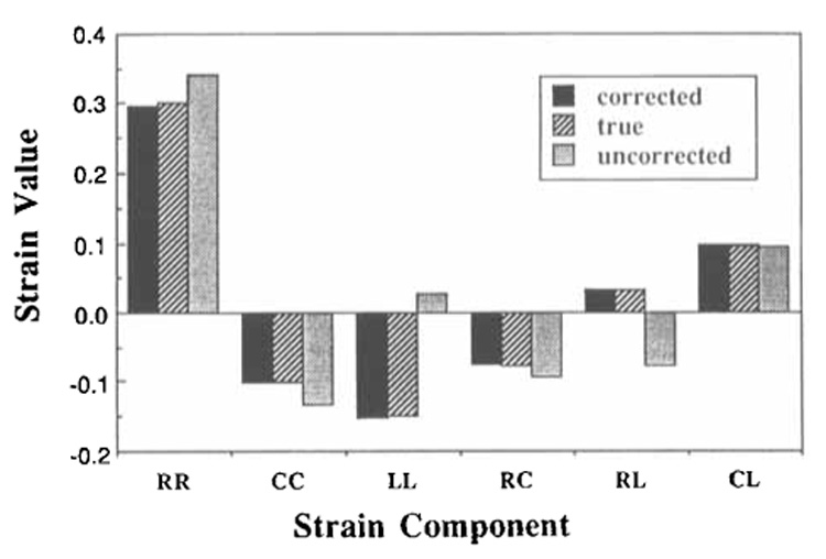
Comparison of corrected strains based on material points, uncorrected strains based on image tag points, and true strains. Strains are from a representative equatorial element of a spherical heart model under approximately physiologic deformations. Note the closeness of the corrected and true strain values, while strains based on image tag points are inaccurate. RR, CC, and LL are axial strain components in the radial, circumferential, and longitudinal dimensions, respectively; RC, RL, and CL are shears. R = radial, outward normal to the epicardial surface of the volume element; C = circumferential; L = longitudinal.

Noise Propagation Analysis

To test for noise propagation through the point-tracking algorithm, a Monte Carlo analysis (20) was done on deforming human heart data. A human heart study was used because of its physiologic geometry. This is important because, for fixed material point errors, the strain error increases with decreasing volume element size. Two-dimensional Gaussian noise was added to all tag points for eight different standard deviations of noise ranging from 0.25 to 2.0 mm (input noise) to model the uncertainty in tag point position. At each input noise level, point tracking was performed for 250 independent trials, and statistics on the material point positions and strains were calculated. All results from the reference and deformed geometries were comparable and conformed to the statistics given below.

The results for material point position error were nearly the same for all material points. For each material point and noise level, the set of error vectors from the trials followed a 3D normal distribution. At a tag point noise level of 2.0 mm, the mean vector of each distribution had a magnitude of less than 0.05 mm, and this magnitude decreased with increasing number of trials. Thus, there was no systematic bias in material point position error.

The standard deviation of the error vector magnitudes in each distribution varied linearly with input noise, reaching 1.5 mm at an input noise level of 2.0 mm. The material point position had a lower uncertainty than the tag point position because of the interpolation used in the algorithm.

The results for strain error were similar for all volume elements. The mean strain errors and standard deviations all varied linearly with input noise level. At an input noise level of 2.0 mm, the mean strain errors of all components were between −.02 and +.02, and the standard deviations were all less than 0.08. The strains with the largest standard deviations were the LL and RL strains.

The relative effects on strain of tag point position uncertainty and of point-tracking interpolation error can be calculated for the deformed spherical heart model. The spherical model was chosen because its large surface curvature aggravates interpolation error. Strain error caused by interpolation was smaller than that from tag point noise when tag point noise exceeded 0.3 mm.

Human Studies

To demonstrate that the algorithm can be applied to tagging data obtained in humans, we imaged a healthy volunteer with the geometry described in “Data Geometry,” according to the following protocol: Standard rotated-phase spin-echo imaging was done with a Signa 1.5-T imager (GE Medical Systems, Milwaukee) with 4.6 version software. The subject was positioned prone on a 5 × 11-inch (12.7 × 27.9-cm) surface coil (GE Medical Systems). The parameters were a TR equal to the RR interval (cardiac gating, average heart rate = 75 beats per minute), a TE of 14 msec (minimum), two signals averaged, a 256 × 128 matrix, and a 30-cm field of view. Short-axis sections were 10 mm thick, with gaps of 2.5 mm. Long-axis sections were 7 mm thick to reduce the saturation near the long-axis line, where the sections intersected.

The tagging pulses began 14 msec after the upslope of the electrocardiograph R wave and had a duration of 12 msec. The 90° pulse of the first image occurred 2 msec after completion of the tagging pulses, and each successive time frame was spaced at 75 msec.

Figure 9 demonstrates the need to account for through-plane motion in human heart studies. The strains are plotted for a typical basal volume element at end systole. Corrected strains are calculated from material points, and uncorrected strains are calculated from short-axis tag points. Note the substantial corrections to the strain obtained with point tracking. Error bars on the corrected strain indicate one standard deviation of the strain error for a tag point noise of 1 mm.

Figure 9.

Comparison of corrected strains based on material points and uncorrected strains based on image tag points for a typical basal volume element (at base of septum) at end systole in a normal human heart. Note the substantial differences, especially in the radial strain, which demonstrate the need to correct for through-plane motion before strain can be accurately calculated. Error bars on the corrected strain indicate one standard deviation of the strain error for a tag point noise of 1 mm.

Figure 10 demonstrates the results of applying the point-tracking and strain calculation methods to a human left ventricle. It shows typical mid—free wall strains at three time points during systole. Note the steady progression in the axial strains (RR, CC, LL) with time and the clear ability to resolve their changes above the maximum expected point-tracking error. The shear strains show more complicated time courses.

Figure 10.

Example of time-resolved 3D strains calculated with the point-tracking technique. Strains are calculated at three time points during systole for a mid-free-wall volume element in a normal human heart. Note the steady progression in the radial thickening (RR) and in circumferential (CC) and longitudinal (LL) contraction strains. The shear strains show a more complicated evolution. Error bars on the corrected strain indicate one standard deviation of the strain error for a tag point noise of 1 mm.

DISCUSSION

Three-dimensional tracking of cardiac motion provides three major benefits. First, it accounts for the substantial through-plane translation of the heart, improving the accuracy of motion and strain calculations. When studying markers at the heart surfaces, as was done here, the changes in heart wall slope and thickness with long-axis position greatly affect the apparent wall thickening on fixed short-axis images. This is the main reason that the radial strain corrections in Figure 9 were so large. With other tag point patterns, such as grids, the radial strain corrections would be smaller.

The second major benefit of 3D tracking is that it allows a more complete evaluation of cardiac mechanics. It accounts for all three motion components, nine deformation gradients, and six strains, compared with just two motions, four deformations, and three strains for 2D tracking. Given the heterogeneous, 3D nature of cardiac deformation, 3D analysis is crucial.

Finally, the method lends itself to the calculation of time-resolved strains, since the same volume of tissue is being examined at every time point.

The interpolation functions used by the point-tracking algorithm required that material point motions be described locally by third-order polynomials. Based on these functions, the algorithm converged rapidly to a unique position for each material point. That these final positions were correct was demonstrated by the accurate tracking of the deforming heart models. The accuracy of interpolation was limited mainly by the number of image planes, the smoothness of the heart wall, and the density of the tag points. The interpolation could be improved by using a more sophisticated interpolation model, such as one based on actual heart contours. This, however, would improve the calculations only if tag point localization was sufficiently accurate to make the interpolation error significant.

Tag point density and tag point uncertainty also have important effects on the strain error. As the density of tag points increases, so does the spatial resolution of the strains. However, as the dimensions of the volume elements decrease, the same uncertainty in tag point position leads to greater strain errors. To improve tag point localization, the optimization of tag profiles, taging/imaging geometries, contouring algorithms, and image signal-to-noise ratio are all important.

The presence of image artifact and stationary blood signal in the left ventricle are the principal obstacles for present contour-detection algorithms. Tag points that lie entirely within the myocardium, defined from striped or intersecting tags, would eliminate the need for an accurate estimate of the endocardial contour. Presaturation techniques could also be used to reduce blood signal intensity inside the left ventricle.

The strains calculated here were based on volume elements with eight vertices instead of the minimum four. This reduces the effect of tag point uncertainty on strain error by least-squares averaging. A problem with the strain tensor used here, however, arises from the homogeneity constraint throughout each volume element, as detailed by Douglas et al (21). Their mathematical models of contracting spherical and cylindric hearts showed substantial radial gradients in strains across the wall, with strains greatest at the endocardium. The generalized inverse method applied here gives representative average strains over each element.

Since the point-tracking method is independent of the subsequent motion or strain analyses, other methods can be applied. A finite-element strain formalism, for example, which we have also implemented but do not present here, can give representative linear transmural strain gradients in circumferential and longitudinal stretches and shears. Transmural gradients of radial strains, however, would require material points within the myocardium and cannot be determined from our data. High-resolution grid tagging permits the definition of material points within the myocardium and may allow such radial strain gradients in wall thickening to be measured (15). Although linear and higher-order approximations to certain transmural strain variations are possible, these measures are inherently more dependent on the accuracy of the tag points.

In conclusion, we have demonstrated several important points: (a) Bulk heart motion through the MR image planes can be substantial; (b) 3D point tracking accounts for the through-plane displacement of the tagged tissue; (c) local, time-resolved 3D strain tensors can be determined with orthogonal stacks of tagged MR images: and (d) tests with deforming cylinders and spheres show that this point-tracking method is accurate and crucial for analyzing cardiac mechanics.

Abbreviations

C

circumferential

L

longitudinal

R

radial

3D

three-dimensional

2D

two-dimensional

APPENDIX

Description of Tracking Algorithm

Definitions

• NLAP: Number of long-axis image planes.

• NSAP: Number of short-axis image planes.

• NSAT: Number of short-axis tag segments (equal to twice the number of short-axis tag planes).

• x_i, y_i, z_i,: Estimated coordinates of the material point at the deformed time, ith iteration (i = 0, 1, 2,….).

• X_Lm, Y_Lm, Z_Lm: Positions of the long-axis tag points from the long-axis tag plane and the heart contour containing the material point being tracked. They are indexed by m, which runs from 1 to 2 × NLAP, since each long-axis plane has two such points on opposite sides of the heart.

• X_CL, Y_CL: The x,y centroid of the long-axis tag points.

• X_Sk, Y_Sk, Z_Sk: Positions of the short-axis tag points of the same tag segment and contour as the material point. There is one such point per short-axis image. They are indexed by k, which runs from 1 to NSAP, to identify the point by its short-axis image plane.

• X_An, Y_An: Coordinates of the tag points in the most apical short-axis image sharing the same contour as the material point. They are indexed by n, which runs from 1 to NSAT, to identify the point by its short-axis tag plane.

• X_Bn, Y_Bn: Same as above, but in the most basal short-axis plane.

• X_CA, Y_CA: The x,y centroid of the above X_An, Y_An points.

• X_CB, Y_CB: The x,y centroid of the above X_Bn, Y_Bn points.

• W_k: Fractional distance from the apical short-axis image plane to the basal short-axis image plane of short-axis image plane k.

• Θ_Sk, R_Sk: Polar coordinates of an X_Sk, Y_Sk tag point with respect to its local origin, indexed by k.

• θ_S, r_S: Polar coordinates of the material point with respect to its local origin, based on the previous (x_t−1, y_t−1) estimate.

• U: Fractional distance from the apical short-axis image plane to the basal short-axis image plane of the plane of the material point at z_t.

The initial position estimate of a material point at a specified time is taken from the short-axis tag point at that time, which has the same short-axis image plane, tag, and contour used to define the material point. Thus, from the tag point we have x₀, y₀, and from the constant z value of this short-axis image plane, we have z₀.

The iteration below is repeated independently for a given material point and a given time. For the ith iteration:

A. Revise z-axis coordinate of material point to reflect through-plane motion.

Using the position estimate of the material point from the previous iteration (x_t−1, y_t−1), find the through-plane motion in this region of the heart by using the tag points in the long-axis images. Since the parallel tags in the long-axis images were all placed coincident with the short-axis image planes on which the material points were initially defined, all material points remain on the deformed long-axis tag surfaces. Thus, the long-axis tag points to be fitted are from the same tag and contour that contain the material point. Their positions are called (X_Lm, Y_Lm), where m is an index to differentiate the long-axis tag points.

To match the geometry of the heart, interpolation is done in polar coordinates. The origin is shifted to the x,y centroid (X_CL, Y_CL) of all the long-axis tag points (X_Lm, Y_Lm) to ensure that their angles are well defined. The following steps are performed:

1. Calculate the x,y centroid of the X_Lm, Y_Lm, tag points for the polar coordinate origin:

$$\begin{array}{c}{X}_{CL}=\sum _{m=1}^{2·\text{NLAP}}\frac{X_{L_m}}{2·\text{NLAP}},\\ Y_{CL}=\sum _{m=1}^{2·\text{NLAP}}\frac{X_{L_m}}{2·\text{NLAP}}.\end{array}$$

2. Shift the tag point coordinates by this centroid origin and rename them $X_{L_m}^{\prime }\text{and}{Y}_{L_m}^{\prime }$:

$$\begin{array}{c}{X}_{L_m}^{\prime }=X_{L_m}-X_{CL},\\ Y_{L_m}^{\prime }=Y_{L_m}-X_{CL}.\end{array}$$

3. Define the angular polar coordinate Θ_Lm for each long-axis tag point:

$${\Theta }_{L_m}=\text{arctan}\left(\frac{Y_{L_m}^{\prime }}{X_{L_m}^{\prime }}\right).$$

4. Fit the z-axis coordinates of these tag points, Z_Lm, with a smooth, periodic, cubic spline as a function of the angles Θ_Lm.

5. Find the angle around the spline, θ_L, at which the z-axis coordinate, Z_t, of the revised material point is to be found:

$${\theta }_L=\text{arctan}\left(\frac{y_{t-1}}{x_{t-1}}\right).$$

6. Evaluate the spline at θ_L, to obtain z_t.

B. Check for convergence.

If |z_t − z_t−1|, > 0.01 mm, go to part C and continue iterating toward the position of the material point. If not, stop iterating and the final position of the material point is x_t−1, y_t−1, z_t.

C. Revise x,y coordinates (x_t, y_t,) of material point.

This is done by interpolating between the short-axis images at the revised z_t level of the material point. The short-axis tag points to be fitted are on the same tag segment and contour as the material point. These are located at X_Sk, Y_Sk, Z_Sk. Cubic spline interpolation is done in polar coordinates with respect to shifted origins to fit these tag points as functions of the z position. To locate these origins, the centroids of the most apical (X_CA, Y_CA) and most basal (X_CB, Y_CB) short-axis images are found by using all tag points with the same contour as the material point. The local tag point origin in each short-axis image plane is the intersection of a straight line between these centroids and the image plane.

1. Calculate centroids of the apical and basal short-axis images:

$$\begin{array}{cc}{X}_{CA}=\sum _{n=1}^{\text{NSAT}}\frac{X_{A_n}}{\text{NSAT}},& Y_{CA}=\sum _{n=1}^{\text{NSAT}}\frac{Y_{A_n}}{\text{NSAT}};\\ X_{CB}=\sum _{n=1}^{\text{NSAT}}\frac{X_{B_n}}{\text{NSAT}},& Y_{CB}=\sum _{n=1}^{\text{NSAT}}\frac{Y_{B_n}}{\text{NSAT}}.\end{array}$$

2. Linearly interpolate in the z dimension between the apical and basal centroids to find local polar origins on the short-axis planes; shift tag point coordinates to local origin. Shifted tag point coordinates are designated $X_{S_k}^{\prime },Y_{S_k}^{\prime }$, and the fractional distance of the short-axis image plane k between the apex and base is W_k:

$$\begin{array}{c}{W}_k=(Z_k-Z_0)/(Z_{\text{NSAP}}-Z_0),\\ X_{S_k}^{\prime }=X_{S_k}-[W_k·X_{CA}-(1-W_k)·X_{CB}],\\ Y_{S_k}^{\prime }=Y_{S_k}-[W_k·Y_{CA}-(1-W_k)·Y_{CB}].\end{array}$$

3. Convert the short-axis tag points to polar coordinates (Θ_Sk, R_Sk):

$$\begin{array}{c}{\Theta }_{S_k}=\text{arctan}\left(\frac{Y_{S_k}^{\prime }}{X_{S_k}^{\prime }}\right),\\ R_{S_k}=\sqrt{{(X_{S_k}^{\prime })}^2+{(Y_{S_k}^{\prime })}^2}.\end{array}$$

4. Independently fit the angles Θ_Sk, and the radii R_Sk with cubic splines as functions of the z-axis coordinate, Z_Sk, of each short-axis image plane.

5. Interpolate to find the angle θ_S, and radius r_S of the material point by evaluating the splines at z_t.

6. Transform the coordinates of the material point back to Cartesian coordinates, with the long axis as the origin. Let U be the fractional distance of the plane of the material point between the apical and basal short-axis imaging planes:

$$\begin{array}{c}U=(z_t-Z_0)/(Z_{\text{NSAP}}-Z_0),\\ x_t=r_s·\text{cos}{\theta }_s+U·X_{CA}+(1-U)·X_{CB},\\ y_t=r_s·\text{sin}{\theta }_s+U·Y_{CA}+(1-U)·Y_{CB}.\end{array}$$

Return to part A of the iteration.

Strain

Description of strain components

Three-dimensional strain is represented as a symmetric 3 × 3 array of numbers, called a tensor, representing the deformation of a body in the three dimensions of a particular orthogonal coordinate system. In this case, we use the radial (R), circumferential (C), and longitudinal (L) dimensions, where radial is defined to be the epicardial outward normal to the particular volume element. Since the tensor is symmetric, there are six unique terms: RR, CC, LL, RC, RL, and CL. Each is labeled by two coordinate dimensions related to the particular type of strain.

These strain terms can be divided into two types: axial and shear. The terms with like coordinates (RR, CC, LL) are axial strains and represent changes in length along that coordinate dimension, normalized by a reference length along that dimension. The strains calculated here are Lagrangian, meaning that the reference length is the undeformed length. Thus, an RR strain would turn a cube (with edges aligned with the axes) into a rectangular block with a different length along the R dimension. Positive axial strains represent extensions, and negative axial strains indicate compressions. The magnitude of the axial strain scales nonlinearly with the fractional change in length. For a uniaxial stretch of 50% (f = 1.5), the axial strain s is calculated from s = 0.5 (f² − 1), so the strain would be 0.625.

The remaining three terms (RC, RL, CL) are shear strains and reflect changes in angles within the volume element. Expressed differently, each term also represents a motion gradient along one of the axes as a function of spacing along the other axis. Thus, in two dimensions, a uniform RC strain would turn a square in the R-C plane into a diamond shape. Positive shears represent a positive motion gradient along one coordinate axis as a function of increasing position along the other axis; negative shears indicate a negative motion gradient along one axis as a function of increasing position along the other axis. Again, the shear strain follows the nonlinear function of the shearing motion gradient.

Strain calculation

A constant 3D strain tensor is calculated in a volume element with the coordinates of its eight material point vertices in the deformed and reference states. The generalized inverse method (21) is used. Since eight material points in a volume element overdetermine a constant 3D strain tensor, the strain values represent a least-squares average strain over the entire element, rather than the strain at any known point. The formalism is straightforward: Given

$$x=F·X,$$

where x is the matrix of the deformed coordinates of the eight material points (3 × 8 matrix), F is the unknown deformation gradient tensor (3 × 3), and X represents the reference material point coordinates (3 × 8), F can be derived by inverting X and postmultiplying both sides of the equation by X inverse. Because X is not a square matrix, it cannot be directly inverted. This is overcome by postmultiplying (F · X) by (X^T · X^−T), where the superscript T indicates transpose and −T the inverse of the transpose:

$$x=F·X·(X^T·X^{-T}).$$

Postmultiplying both sides by X^T, we have

$$x·X^T=F·X·X^T.$$

Finally, after postmultiplying both sides by (X · X^T)⁻¹, where X · X^T is square (3 × 3) and invertible, F is obtained:

$$F=x·X^T·{\left(X{·X}^T\right)}^{-1}.$$

The Lagrangian finite strain tensor E is then computed from F:

$$E=½(F^T·F-I)$$

where I is the identity matrix.

References

- 1.Hunter WC, Zerhouni EA. Imaging distinct points in left ventricular myocardium to study regional wall deformation. In: Anderson JH, editor. Innovations in diagnostic radiology. Berlin: Springer-Verlag; 1989. pp. 169–190. [Google Scholar]
- 2.Arts T, Reneman R, Veenstra P. A model of the mechanics of the left ventricle. Ann Biomed Eng. 1979;7:299–318. doi: 10.1007/BF02364118. [DOI] [PubMed] [Google Scholar]
- 3.Arts T, Meerbaum S, Reneman R, Corday E. Torsion of the left ventricle during the ejection phase in the intact dog. Cardiovasc Res. 1984;18:183–193. doi: 10.1093/cvr/18.3.183. [DOI] [PubMed] [Google Scholar]
- 4.Guccione JM, McCulloch AD. Finite element modeling of ventricular mechanics. In: Glass L, Hunter P, McColluch A, editors. Theory of heart: biomechanics, biophysics, and non-linear dynamics of cardiac function. New York: Springer-Verlag; 1991. pp. 121–144. [Google Scholar]
- 5.Douglas AS, Rodriguez EK, O'Dell WG, Hunter WC. Unique strain history during ejection in canine left ventricle. Am J Physiol. 1991;260:H1596–H1611. doi: 10.1152/ajpheart.1991.260.5.H1596. [DOI] [PubMed] [Google Scholar]
- 6.McCulloch AD, Smail BH, Hunter PJ. Regional left ventricular epicardial deformation in the passive dog heart. Circ Res. 1989;64:721–733. doi: 10.1161/01.res.64.4.721. [DOI] [PubMed] [Google Scholar]
- 7.Waldman LK, Fung YC, Covell JW. Transmural myocardial deformation in the canine left ventricle. Circ Res. 1985;57:152–163. doi: 10.1161/01.res.57.1.152. [DOI] [PubMed] [Google Scholar]
- 8.Hansen D, Daughters G, Alderman E, Ingels N, Jr, Miller DC. Torsional deformation of the left ventricular midwall in human hearts with intramyocardial markers: regional heterogeneity and sensitivity to the inotropic effects of abrupt rate changes. Circ Res. 1988;62:941–952. doi: 10.1161/01.res.62.5.941. [DOI] [PubMed] [Google Scholar]
- 9.Zerhouni EA, Parish DM, Rogers WJ, Yang A, Shapiro EP. Human heart: tagging with MR imaging—a method for noninvasive assessment of myocardial motion. Radiology. 1988;169:59–63. doi: 10.1148/radiology.169.1.3420283. [DOI] [PubMed] [Google Scholar]
- 10.Axel L, Dougherty L. Heart wall motion: improved method of spatial modulation of magnetization of MR imaging. Radiology. 1989;172:349–350. doi: 10.1148/radiology.172.2.2748813. [DOI] [PubMed] [Google Scholar]
- 11.Axel L, Dougherty L. MR imaging of motion with spatial modulation of magnetization. Radiology. 1989;171:841–845. doi: 10.1148/radiology.171.3.2717762. [DOI] [PubMed] [Google Scholar]
- 12.McVeigh ER, Zerhouni EA. Book of abstracts: Society of Magnetic Resonance in Medicine 1989. Vol. 53. Berkeley, Calif.: Society of Magnetic Resonance in Medicine; 1989. A rapid starburst sequence for cardiac tagging (abstr) [Google Scholar]
- 13.Bolster BD, McVeigh ER, Zerhouni EA. Myocardial tagging in polar coordinates with striped tags. Radiology. 1990;177:769–772. doi: 10.1148/radiology.177.3.2243987. [DOI] [PMC free article] [PubMed] [Google Scholar]
- 14.Mosher TJ, Smith MB. A DANTE tagging sequence for the evaluation of translational sample motion. Magn Reson Med. 1990;15:334–339. doi: 10.1002/mrm.1910150215. [DOI] [PubMed] [Google Scholar]
- 15.McVeigh ER, Zerhouni EA. Noninvasive measurement of transmural gradients in myocardial strain with MR imaging. Radiology. 1991;180:677–683. doi: 10.1148/radiology.180.3.1871278. [DOI] [PMC free article] [PubMed] [Google Scholar]
- 16.Guttman M, Prince J. Image analysis methods for tagged MRI cardiac studies. SPIE Roc Med Imaging. 1990:1233–1218. [Google Scholar]
- 17.Pipe JG, Boes JL, Chenevert TL. Method for measuring three-dimensional motion with tagged MR imaging. Radiology. 1991;181:591–595. doi: 10.1148/radiology.181.2.1924810. [DOI] [PubMed] [Google Scholar]
- 18.Pelc NJ. Book of abstracts: Society of Magnetic Resonance in Medicine 1991. Vol. 17. Berkeley, Calif.: Society of Magnetic Resonance in Medicine; 1991. Myocardial motion analysis with phase contrast cine MRI (abstr) [Google Scholar]
- 19.Rogers WJ, Shapiro EP, Weiss JL, et al. Quantification of and correction for left ventricular systolic long-axis shortening by magnetic resonance tissue tagging and slice isolation. Circulation. 1991;84:721–731. doi: 10.1161/01.cir.84.2.721. [DOI] [PubMed] [Google Scholar]
- 20.Press W, Flannery B, Teukolsky S, Vetterling W. Numerical recipes in C: the art of scientific computing. Cambridge, England: Cambridge University Press; 1988. pp. 548–557. [Google Scholar]
- 21.Douglas AS, Hunter WC, Wiseman MD. Inhomogeneous deformation as a source of error in strain measurements derived from implanted markers in the canine left ventricle. J Biomech. 1990;23:331–341. doi: 10.1016/0021-9290(90)90061-7. [DOI] [PubMed] [Google Scholar]