Four-dimensional B-spline based motion analysis of tagged MR images

Abstract

In MRI tagging, magnetic tags—spatially encoded magnetic saturation planes—are created within tissues acting as temporary markers. Their deformation pattern provides useful qualitative and quantitative information about the functional properties of underlying tissue and allows non-invasive analysis of mechanical function. The measured displacement at a given tag point contains only unidirectional information; in order to track the full 3D motion, these data have to be combined with information from other orthogonal tag sets over all time frames. Here, we provide a method to describe the motion of the heart using a four-dimensional tensor product of B-splines. In vivo validation of this tracking algorithm is performed using different tagging sets on the same heart. Using the validation results, the appropriate control point density was determined for normal cardiac motion tracking. Since our motion fields are parametric and based on an image plane based Cartesian coordinate system, trajectories or other derived values (velocity, acceleration, strains...) can be calculated for any desired point within the volume spanned by the control points. This method does not rely on specific chamber geometry, so the motion of any tagged structure can be tracked. Examples of displacement and strain analysis for both ventricles are also presented.

1. Introduction and background

1.1. Motivation

Cardiovascular diseases are the primary cause of mortality in the developed world; therefore development of better functional cardiac imaging techniques in the hope of achieving early diagnosis and better follow up is a very active research area. Main 3D and 4D (3D + time) cardiac imaging modalities are ultrasound (US), computed tomography (CT), nuclear medicine (e.g. gated SPECT) and magnetic resonance imaging (MRI). Advantages of MRI are high spatial resolution, excellent soft tissue contrast, intrinsic 3D acquisition and absence of ionizing radiation. In recent years, with the rapid development of new MRI techniques, a complete MR-based cardiac evaluation is becoming a reality (McVeigh 1998). This includes the assessment of local and global mechanical function, chamber morphology, blood flow, myocardial perfusion, coronary circulation and MR spectroscopy. Our focus in this paper is the assessment of cardiac mechanical function using MRI tagging.

1.2. Tagged MRI, background

One of the techniques used for the analysis of cardiac mechanics is tagged MRI. MRI imaging is based on selectively disturbing tissue magnetization in a high magnetic field and observing the resulting inductive effects. Tags are voids in the regular MRI images created by spatially selective presaturation pulses (figure 1). These move with the tissue and provide temporary internal fiducial markers. Tagging was originally proposed by Zerhouni et al (1988) and was followed by several efforts to produce tags faster or in a more versatile way (Axel and Dougherty 1989, Mosher and Smith 1990, McVeigh and Bolster 1998). The measured tag deformation at a single tag point contains only a unidirectional component of its past motion, from tagging to imaging time. In order to achieve a full 3D tracking of any point through time, the information coming from different tagging sets has to be combined and interpolated in space and time (figure 2). At least three independent tagging directions are necessary to reconstruct the motion in 3D. Here we provide a stepwise method to achieve a 4D representation of cardiac motion starting from a set of tagged MRI images.

Figure 1.

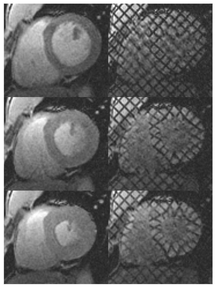
Left: standard cardiac MR images. Right: for the same heart, location and cardiac phase, the corresponding tagged MR images. Top: at end-diastole, when the ventricular cavity is at its maximum filling, right after tagging. Middle: At mid-systole, when the heart is contracting. Bottom: at end-systole, when the maximum amount of blood has been ejected and the heart muscle is at its maximum contraction.

Figure 2.

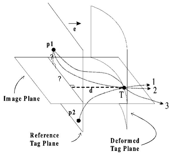
The tag point displacement d, which is measured at the tag point T at a given time, gives only one component of the past trajectory, so it cannot be mapped back uniquely. For example, point T might originate from p1, or from p2. The correct matching point p1 at the undeformed state (at tagging time) can only be found by incorporating the tag displacement information coming from other tag planes. Using all tags at a given time frame, we can locate point p1, but we cannot be sure of its trajectory (lines 2 and 3 are two of the many possible paths). Using the matching points at every time frame we calculate a final forward motion field and find the correct trajectory.

1.3. Tagged MRI based motion analysis

Previously, several methods have been developed to analyse tagged MR images. Some of them rely on specific geometry of the chambers and require careful alignment of a specific coordinate system (O’Dell et al 1995, Declerck et al 1999). Other techniques rely on finite element models (Young and Axel 1995, Young et al 1995), or finite difference analysis for a fixed number of vertices (Denney and McVeigh 1997). For a detailed comparison of several approaches to motion analysis of tagged MRI images, the reader is referred to another paper in this issue (Declerck 2000).

1.4. B-spline based tagged MRI analysis

An advantage of using piece-wise polynomial functions to describe the tissue deformation is the absence of ringing problems of global polynomial fitting. B-splines become a good candidate, since they cannot only describe one-dimensional tag displacements, but also characterize deformations for the image plane, volume-of-interest or space-time continuum as tensor products.

B-splines are widely used in computer graphics for curve and surface representations (de Boer 1998). They have several very useful properties: parametric continuity, compact representation of the information, local support and differentiability (Daniel 1996, Farin 1990).

Several B-spline based techniques have been employed in the past to describe deformed tags: Moulton et al (1996) utilized them to describe the deformed tag planes as surfaces, but they used a global polynomial basis function expansion for the final forward tracking. In the first approach of Amini et al (1998) tags were segmented using a two-dimensional coupled B-snake grid, but no parametric motion field was constructed for the material points. In that study, to get the displacement information at any other image point a thin-plate spline based finite difference method has been proposed. They later provided a general framework for the extension of their approach to 3D (Radeva et al 1997). Although their method and ours use the same B-spline concept, there are several differences: (a) we employ a different parametrization method and (b) our starting point for the analysis is segmented tag points not images, so we need a separate tag segmentation algorithm. These issues will be addressed further in section 5.

We have previously introduced our approach to cardiac motion tracking (Ozturk and McVeigh 1999). In this paper we provide the following: (a) in vivo validation of our motion tracking algorithm and determination of the appropriate control point density for normal cardiac motion; (b) refinement and complete description of our tag displacement and forward motion field fitting algorithms; (c) improvement and validation of through plane motion field fitting; (d) examples of left and right ventricular motion analysis.

This paper is organized as follows. In section 2 the imaging protocol and some of the mathematical details are given. Section 3 includes the results for in vivo validation. Section 4 contains sample displacement and strain analysis for the left and right ventricle under normal and pathological conditions. The discussion (section 5) is followed by a final summary. The appendix contains some further mathematical details of the least square method used when calculating the control points.

2. Methods

A cardiac tagged MRI study can be divided into several steps: (a) tagging and fast MR imaging, (b) segmentation of myocardium and tag detection, (c) registration and combination of information from different tagging directions, (d) tag displacement field fitting for each imaging plane, tagging direction and time frame, (e) combining of all displacement fields to an inverse motion field and sampling of this field giving matching pairs of points between later time frames and the undeformed state and (e) forward motion field fitting to track cardiac points from tagging time on.

2.1. Imaging protocol

MR images were acquired from a healthy volunteer using a breath-hold SPGR cine acquisition (McVeigh and Atalar 1992) and a dedicated Cardiac 1.5T GE Signa scanner. We obtained two separate tagging data sets from the same heart. Each data set is adequate by itself for cardiac motion tracking but the sets will be used to validate each other. These sets will be referred to as set1 and set2 in the remainder of this article (and with an index s in the formulae). For each set the same short-axis (SA) planes are used and cine images (11 cardiac phases) are acquired with a grid tagging pattern, rotated 45 degrees between two sets (figure 3). A group of parallel tag planes forms a tag stack; SA images of each set contain tag displacement information coming from two tag stacks. Tag planes are initially arranged perpendicular to the imaging plane; they deform over time and intersect the SA imaging planes forming tag lines. For each set, six long-axis (LA) images are acquired perpendicular to SA images, every 30 degrees around the left ventricle long axis. Please note that, in contrast to SA, the locations of LA image planes are different for both sets (figure 4). For all LA images, tag stacks are arranged in a way that one of the stacks provided the displacement information orthogonal to both SA tag stacks (figure 5).

Figure 3.

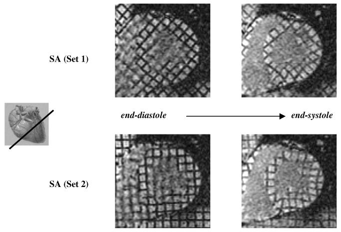
Top: SA slice of set1 at end-systole (right) and end-diastole (left) with diagonal tagging. Bottom: same image location but tagged in the horizontal-vertical grid pattern giving the corresponding images of set2.

Figure 4.

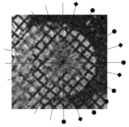
Long-axis image locations for both sets displayed on a sample short-axis slice. Set1 (◆), set2 (●). Each set is composed of six slices arranged radially around the left ventricle’s long axis and both sets interleave each other.

Figure 5.

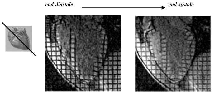
A sample long axis image at end-diastole (left) and end-systole (right).

MR imaging parameters employed during the validation part of the study were as follows: TR = 6.4-6.6 ms, TE = 1.7 ms, flip angle= 10°, 256 frequency encoding steps, 192 phase encoding steps, field of view 32 × 24 cm, slice thickness 8 mm, eight phase encoding steps per cardiac phase (NVP), tag spacing 7.5 mm (six pixels), and an effective voxel size of 1.25 × 1.25 × 8 mm. Nine SA slices and six LA slices at were acquired eleven cardiac phases. Each set consisted of 99 SA images and 66 LA images. The first time frame was 10 ms after the tagging time.

2.2. Segmentation, tag detection and registration

In each image, endo- and epicardial contours of the left ventricle were outlined semiautomatically using the Findtags program of Guttman et al (1997). If necessary, for right ventricular delineation an in-house developed program (GContour) was used to manually segment both ventricles. Once the myocardium was segmented, points on tags are detected automatically using the active tag detection algorithm of Findtags (Guttman et al 1994). The physical location and time stamp of each image is known from the imaging protocol, so tag points can be registered easily in 3D space and within the cardiac cycle. All of the detected tag points are converted to an image-based coordinate system formed by the two SA tag directions of the first set and the SA image normal.

2.3. Inverse motion field fitting

For a given tagging set (s), short-axis plane (j) and time frame (i), we have separate displacement information coming from two tag stacks. For each tag stack (k), segmented tag points can be further addressed by two more indexes; the first one identifying to which tag plane they belong (l) and the second one representing their location along a given tag line (m). Using this notation the tag displacement d at a tag point T can be written as

$$d_{i,j,k,l,m}^{\left(s\right)}=({\overrightarrow{T}}_{i,j,k,l,m}^{\left(s\right)}-{\overrightarrow{P}}_{0,k,l}^{\left(s\right)})•{\overrightarrow{N}}_k^{\left(s\right)}$$ (1)

where i is the time frame number (1 ≤ i ≤ 11), j is the short-axis the image plane number (1 ≤ j ≤ 9), k is the tag stack number (1 ≤ k ≤ 2), l is the tag plane index number, m is the point number along the tag line, s is the set index (s = 1 or s = 2), P_0,k,l is a point on tag plane l of stack k at tagging time, N_k is the unit normal of the tag plane k and (●) is the dot product.

Each tag point T has three coordinates in the new image based coordinate system. For each SA plane, time frame and SA tag stack of a given set, we formulate a two-dimensional B-spline tensor field:

$${\widehat{d}}_{i,j,k}^{\left(s\right)}=\sum _u\sum _v{B}_u\left(x\right)B_v\left(y\right)C_{i,j,k,u,v}^{\left(s\right)}.$$ (2)

In the above equation B is the B-spline basis function, x and y are image coordinates, u and v are B-spline parameters and C are control point values. Summation is done over all the defined control point 2D tensor products for a given xy-location. The basis function for a given location is calculated from the homogeneous knot sequence of the corresponding desired control point number and degree of the B-spline using the standard iterative formula (de Boer 1978). We have chosen cubic splines and several densities of 2D control point grids have been employed. The control points for a given SA image plane, tag direction and time frame are determined using least squares with peripheral conditioning (see the appendix). Since there are eleven time frames, nine SA image planes and two SA tag stacks, 198 independent tag displacement fields are computed for each set.

We have a B-spline parametric representation, so we can calculate the tag displacement value at any image point using equation (2). If we evaluate the field at the original tag points, we can compute the absolute difference between calculated and observed displacements as the tag displacement residual error. This was done for a range of control point densities (section 3).

After calculating displacement fields of both tag stacks at a given SA image plane and time frame, we can determine two components of the past total trajectory of any tag point. If care is taken to use the same region of interest in both SA tag displacement fields for a given SA image, we can describe a single 2D inverse deformation field (U):

$$\begin{array}{c}{U}_{i,j}^s:{\mathfrak{R}}^2\to {\mathfrak{R}}^2\hfill \\ {\overrightarrow{D}}_{i,j}^{\left(s\right)}=\sum _u\sum _v{B}_u\left(x\right)B_v\left(y\right)\left[\begin{array}{c}\hfill C_{i,j,1,u,v}^{\left(s\right)}\hfill \\ \hfill C_{i,j,2,u,v}^{\left(s\right)}\hfill \end{array}\right].\hfill \end{array}$$ (3)

This is similar to equation (2), but the final displacement is now a 2D vector. For any point, at a given SA image plane and time frame, the result of this inverse field is a 2D vector pointing to the planar projection of its reference point (at tagging time) to the current image plane. Since there are two separate sets, we have two distinct 2D inverse fields at each SA imaging plane.

For cross validation of the SA inverse fields, the inverse 2D deformation calculated from one set will be evaluated at the tag points of the second set (figure 6). Using the inverse fields derived from one set, tag displacement at the tag points of the other set can be calculated directly:

$$\begin{array}{c}\hfill {\widehat{d}}_{i,j,k,l,m}^{\left(1\right)}=U_{i,j}^{\left(2\right)}\left(T_{i,j,k,l,m}^{\left(1\right)}\right)•N_{i,j,k}^{\left(1\right)}\hfill \\ \hfill {\widehat{d}}_{i,j,k,l,m}^{\left(2\right)}=U_{i,j}^{\left(1\right)}\left(T_{i,j,k,l,m}^{\left(2\right)}\right)•N_{i,j,k}^{\left(2\right)}\hfill \end{array}$$ (4)

where N is the unit tag normal and U is the 2D inverse field function as defined by equation (3). The difference between the observed and calculated displacements—when calculation is done using the other set’s inverse motion parameters—is defined as the validation error of the SA tag displacement field.

Figure 6.

Top row: original tag displacements of set1 (left) and set2 (right) at a sample short axis plane. Middle row: displacements at tag points for both sets, calculated using the inverse field parameters of the same set. Bottom row left: displacement values at tag locations of set1, calculated using the displacement field parameters of set2. Bottom row right: tag displacements of set2 using the parameters of set1.

2.4. Through plane motion field fitting

The final inverse motion field should map each tag point to its reference location at the undeformed state (tagging time). The missing component of equation (3) is the SA through-plane motion, which can be computed using LA images. This process involves these additional steps:

• Step 1: 2D B-spline field fit for the tag displacement at each LA plane.

• Step 2: Evaluation of the LA parametric fields at each SA image plane intersection line.

• Step 3: A field fit at each SA plane using the through-plane motion information coming from step 2.

The first and last steps are essentially identical to SA tag displacement field fitting of section 2.2. At the end of step 2, we have a radial sampling of through-plane motion at SA imaging planes (Ozturk and McVeigh 1999). We can now describe a 3D inverse field:

$$\begin{array}{c}{U}_{i,j}^s:{\mathfrak{R}}^2\to {\mathfrak{R}}^3\hfill \\ {\overrightarrow{D}}_{i,j}^s=\sum _u\sum _v{B}_u\left(x\right)B_v\left(y\right)\left[\begin{array}{c}\hfill C_{i,j,1,u,v}^{\left(s\right)}\hfill \\ \hfill C_{i,j,2,u,v}^{\left(s\right)}\hfill \\ \hfill C_{i,j,3,u,v}^{\left(s\right)}\hfill \end{array}\right].\hfill \end{array}$$ (5)

The validation of through-plane motion is slightly different, since we no longer have two independent tagging sets at every imaging plane. We calculate the through-plane errors at SA imaging planes using the z component of equation (5). The residual error is the difference between the calculated and original through plane values for each set (radial sampled information at the end of step 2 above). For the calculation of the validation error set1 we evaluate the through plane field at the locations of set2, and for set2 at locations of set1.

2.5. Forward motion field fitting

A common difficulty in understanding cardiac tagging is description of the motion of the heart in material coordinates. Since imaging planes are fixed and the heart is moving in and out of this plane during imaging, tag displacements measured at the same image location but at different time frames point back to different cardiac material points. We define the cardiac material points by their positions in a volume of interest at the tagging time.

Three-dimensional inverse displacement vectors of all the corresponding SA tag points are calculated using equation (5) for each set. These displacement vectors map tag points to their material locations at tagging time. Conversely, for every time frame, the forward transformation should bring the material points back to their corresponding tag point locations. The forward deformation for a given time frame (i) of a set (s) can be described as a three-dimensional B-spline tensor product:

$${\varphi }^s\left(P_i\right)=\sum _u\sum _v\sum _w{B}_u\left({\tilde{x}}_i\right)B_v\left({\tilde{y}}_i\right)B_w\left({\tilde{z}}_i\right){\overrightarrow{C}}_{u,v,w,i}^{\left(s\right)}.$$ (6)

In this equation, the sum for a given material is done over the 3D tensor product of basis functions and control points. The basis functions for a given location are calculated, as before, using the corresponding knot sequence and degree of the B-spline. We distinguish material from image based coordinates with the use of the symbol (∼). Please note that the result of this motion field is not the coordinates of the new location but a vector pointing to the new location from the material point P. Control points for each time frame are found by least-squares minimization. After the 3D forward deformation field is constructed for each time frame, a smoothing of control point values is performed over time. For this we have used cubic splines and seven control points. Time smoothing parameters have been kept constant when different densities of spatial control points were evaluated. At the end, we describe the motion of the heart for each set as a four-dimensional B-spline forward motion field:

$${\varphi }^s(\overrightarrow{P},t)=\sum _u\sum _v\sum _w\sum _t{B}_u\left(\tilde{x}\right)B_v\left(\tilde{y}\right)B_w\left(\tilde{z}\right)B_t\left(t\right){\overrightarrow{C}}_{u,v,w,t}^{\left(s\right)}.$$ (7)

We similarly define two measures to evaluate the accuracy of the final forward motion field. The first one is the forward field residual error, which is the 3D distance between the original tag point and the position to which that tag point is mapped following its inverse and forward transformations. The forward field validation error is calculated the same way, but after inverse transforming the tag points of set1 we use the forward field parameters of set2. Similarly for set2 points we use set1’s forward field.

2.6. Generation of synthetic tags

In the evaluation of the final motion field, it is useful to deform and follow synthetic tag planes from tagging time on. We can intersect these deformed tag planes with imaging planes and compare these artificial tag lines with the original tag points. Since we only have a 4D forward representation, the material point that maps to a specific tag point location at a later time frame cannot be calculated directly. Using coordinate transformations we have converted this problem to a simple 2D interpolation (Ozturk and McVeigh 1999). Since we could also create synthetic tags using the forward motion field of the other set we could have two synthetic tags for any original tags.

2.7. Endo and epicardial surface fitting

Cardiac contours are not necessary in our motion field calculations, but they are used for tag segmentation. They are also useful in the display of the results. Our 2D B-spline approach can be modified to represent the endo and epicardial contours of the heart:

$$\begin{array}{c}{S}^i:{\mathfrak{R}}^2\to {\mathfrak{R}}^3\hfill \\ A=\sum _u\sum _v{B}_u\left(l\right)B_v\left(z\right){\overrightarrow{C}}_{u,v}\hfill \end{array}$$ (8)

In equation (8), B is the B-spline basis function and C is the 3D control points of the surface. The summation is done over the 2D tensor product of basis functions. The surface is designated with two parameters: z and l. z is the parametrization perpendicular to SA imaging planes, so every contour point in an SA image plane has the same z value. The second parameter l is a chord length parametrization along the contours:

$$l\left(k\right)=\frac{\sum _{i=2}^k\parallel (P_i-P_{i-1})\parallel }{\sum _{i=2}^n\parallel (P_i-P_{i-1})\parallel }$$ (9)

where k is an index of points along the contours and n is the total number of points in a given contour line, making the denominator of equation (9) the total length of the curve. For the initial point, l(1) = 0. Since contours can be open or closed (e.g. right and left ventricular contours respectively), necessary changes have been made to equation (9) to incorporate circularity when needed. To prevent twisting of the closed surfaces, the chord length parametrization of subsequent slices has to be adjusted to compensate for the in-plane shift of the starting point.

For a given choice of control point density, the control points are found by least-squares minimization of

$$E=\sum _i\sum _j\left({\Vert P_{i,j}-\left(\sum _u\sum _v{B}_u\left(z_{i,j}\right)B_v\left(l_{i,j}\right)C_{u,v}\right)\Vert }^2\right).$$ (10)

Once control points are found for endo- and epicardial surfaces homogeneous sampling of this surface will give a uniform surface mesh, which can be deformed by the previously calculated motion field and displacement and strain values can be mapped on the mesh for display (see section 4).

2.8. Strain calculation

We have a parametric representation of the material coordinate displacement field (equation (7)). The displacement gradient can be computed at each point

$$g_{i,j}(\tilde{x},\tilde{y},\tilde{z})=\frac{\partial U_i}{\partial X_j}$$ (11)

where U_i is the ith component of the material displacement field as calculated by equation (7) and X is the material coordinate position vector. Equation (7) can be differentiated directly using properties of the B-spline basis function. For example:

$$g_{x,x}=\sum _u\sum _v\sum _w\sum _t{B}_u^{\prime }\left(\tilde{x}\right)B_v\left(\tilde{y}\right)B_w\left(\tilde{z}\right)B_t\left(t\right)C_{u,v,w,t}^{\prime }$$ (12)

where B′ is the derivative of the B-spline basis function. The derivative of a cubic B-spline with a knot sequence

$$\begin{array}{cc}\hfill K=\{0,0,0,u_1\dots u_k\dots u_{k-3},1,1,1,1\}\hfill & \hfill \text{where}{u}_n=n∕(k-2)\hfill \\ \hfill \text{for}1\le n\le (k-3).\hfill & \hfill \hfill \end{array}$$

can be calculated directly as the quadratic B-spline of the shortened knot sequence:

$$\begin{array}{cc}\hfill K^{\prime }=\{0,0,0,u_1\dots u_k\dots u_{k-3},1,1,1,1\}\hfill & \hfill \text{where}{u}_n=n∕(k-2)\hfill \\ \hfill \text{for}1\le n\le (k-3).\hfill & \hfill \hfill \end{array}$$

The tensor product for the desired displacement gradient component for the whole space is done as before with the difference that the basis in the x direction is now quadratic. The new control points can be computed from the old ones as:

$$C_{u,v,w,t}^{\prime }=p\frac{C_{u+1,v,w,t}-C_{u,v,w,t}}{K_{i+p+1}-K_{i+1}}$$

where p is the degree of the B-spline (p = 3 for our case) and K is the original knot sequence in the x direction. The remaining eight components of the displacement gradient tensor can be similarly described analytically. The local Lagrangian strain tensor at any location (Spencer 1980), ε, can then be computed from the displacement gradient, g, using the formula

$$\epsilon =\frac{1}{2}(g^T+g+g^{T}g).$$ (13)

The strain once computed can be transformed to a local surface based coordinate system to display circumferential, radial and longitudinal components.

3. In vivo validation results

The validation of our motion analysis method will be done for each step. First, the inverse tag displacement field fitting process will be evaluated for the SA imaging planes, second the accuracy of the through-plane displacement field will be examined. The forward motion fields will be validated at the end. At each step, several densities of control points will be used to explore the relationship between the choice of parameters and the accuracy.

3.1. SA tag displacement field fitting

For all SA image planes, original tag displacements are compared with the calculated values using the inverse field parameters of the same (residual error) and opposite set (validation error) (figure 6). For each set and tag stack, tag displacement errors show a steady increase through systole reaching a maximum value for time frame 10 (end systole). No significant residual or validation error difference was observed between individual SA slices.

The end systolic residual error of all four SA tagging directions is shown in figure 7 for several choices of control point densities. For all tag orientations the residual error displayed a steady decline for the calculated range of control point densities. No significant difference was present between different sets or tag orientations.

Figure 7.

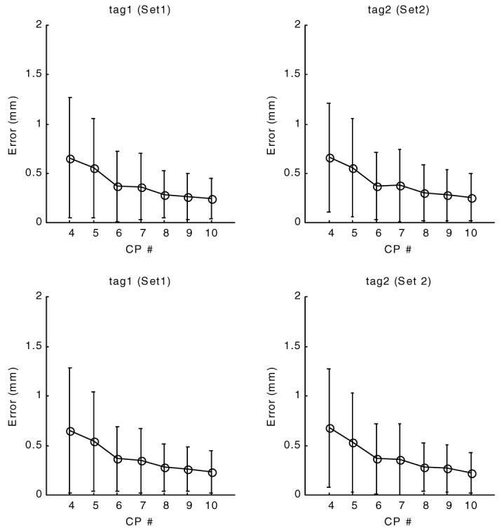
Residual error of tag displacement field fit for short-axis tags at end systole (time frame 10). The x-axis is the planar control point density, 4 represents a 4 by 4 control point array. The y-axis displays the mean and standard deviation of the residual error, the difference between calculated and observed tag displacements.

The validation errors (figure 8) exhibited an early decrease with increasing control point density, but reach a plateau around 0.75 mm (0.6 pixels). No significant difference was observed when set1 derived fields were applied on points of set2 or set2 fields were applied on set1’s points.

Figure 8.

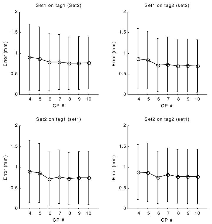
Validation error of tag displacement field at end systole (time frame 10). The x-axis is the planar control point density. The y-axis displays the validation error, the difference between calculated and observed tag displacements. In contrast to figure 7, the displacement values for set1 tag points are calculated using the field parameters of set2, and vice versa.

3.2. Through-plane displacement field fitting

Two different through-plane motion fields can be computed from two LA sets at each SA imaging plane. The combined residual and validation errors of through-plane motion are displayed in figure 9 for time frame 10 (end systole). The residual error showed a steady decline for the calculated range of control point densities. The validation errors, on the other hand, reached a quick plateau around 0.4 mm. The LA tag displacement field control point density (8 × 8) and SA plane sampling densities (every 1 mm) were kept constant during the through-plane motion field experiments (Steps 1 and 2 of section 2.4). No significant difference was present between the results of different sets.

Figure 9.

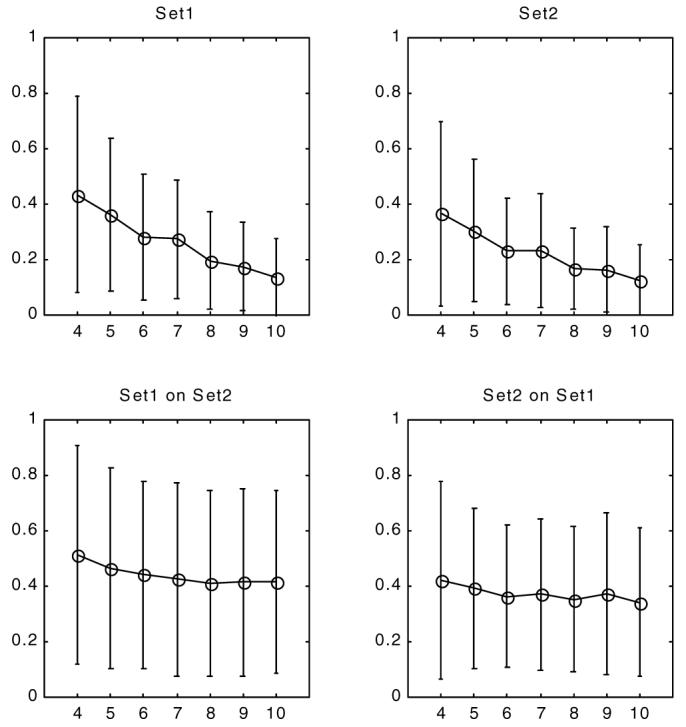
Residual (top) and validation (bottom) errors of through plane displacement field at end systole (time frame 10) for both sets. The x-axis is the planar control point density. the y-axis is the absolute displacement error (in mm) calculated over all slices. For validation to compute the displacement at the locations of a given set we use the parameters of the other set.

3.3. Forward field fitting

For all forward field analysis, a fixed inverse field control point density of 8 by 8 was used at both SA and LA image planes. Forward field computation uses the matching points between tagging and later time frames which is calculated using the 3D inverse field. For four-dimensional analysis a time smoothing is done separately over each 3D control point value over time. We chose cubic B-splines with a time control point density of 7 for time smoothing.

Residual and validation forward errors are given in figures 10 and 11 for different choices of control point density at time frame 10. Similar to the inverse field errors, the residual errors of the forward field fitting displayed a steady decline for the given range of control point densities for both sets and for 3D or 4D.

Figure 10.

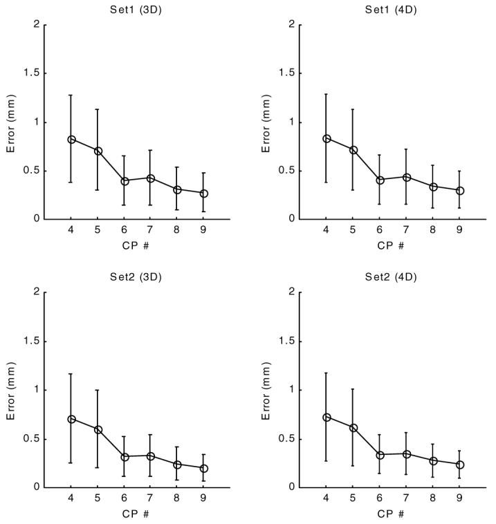
Residual error of forward motion field at end systole (time frame 10). The x-axis is the control point density, 4 represents a 4 by 4 by 4 control point array (or 4 by 4 by 4 by 7 for 4D). The y-axis is the residual error, the difference between calculated and original tag locations. The calculated location of a tag point is found by first mapping it to the matching point at tagging time (3D inverse field) and bringing that point back using the forward transformation (using either a 3D or 4D version).

Figure 11.

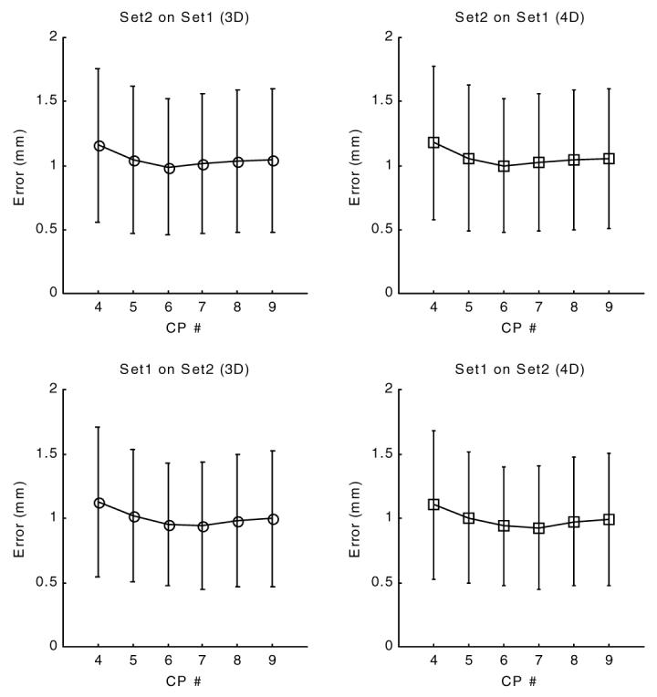
Validation error of forward motion field at end systole (time frame 10). The x-axis is the control point density and the y-axis displays the validation error, the 3D distance between the original tag point and the final position after applying first an inverse then a forward transformation. In contrast to figure 10, the forward transformation at locations of set1 was computed using the parameters of set2 and for locations of set2 we used parameters of set1.

The validation error of forward transformation (figure 11) showed an initial decline, reached a minimum value around 1.1 mm (less than one pixel) for a control point density of 6 × 6 × 6 and displayed a slight increase with further increase of control point density.

4. Analysis of the dynamics of both ventricles

The strength of our method comes from the model-free approach in field fitting. Therefore, in this section, examples of the displacement and strain analysis for left and right ventricles are given. The images in this part are acquired using the same imaging protocol as used in the human studies above (section 2.1); however, a canine dataset was chosen because it provided much better details in the RV.

In figure 12, cine MR images of a selected slice of a normal canine heart are displayed with original and synthetic tag lines. The synthetic tag lines were calculated, as described in section 2.5, from the final forward motion field. For the same imaging plane, inverse displacements and principal strains are shown on a homogeneous grid on the myocardium (figure 13). For each location the 3D inverse displacement vector points to the corresponding position at tagging time. The contraction and normal twisting of the left ventricle can be easily observed. On the right column of Figure 13, two principal strain directions at each location are represented by line segments, the length of which is proportional to their corresponding eigenvalues. The principle strains were calculated from the Lagrangian strain tensor that is computed from the local deformation gradient (see section 2.8). A 3 × 3 symmetric strain tensor matrix can always be decomposed mathematically to its eigenvalues and eigenvectors. The maximum and minimum eigenvalues will then represent respectively the amplitude of the main stretch and shortening along the corresponding eigenvector directions. In figure 13 (left column), only the maximum and minimum eigenvectors are displayed; for the LV, the eigenvectors at later time frames corresponding to the smallest eigenvector display mainly circumferential shortening, whereas the maximum eigenvectors are arranged in radial directions, representing a local wall thickening.

Figure 12.

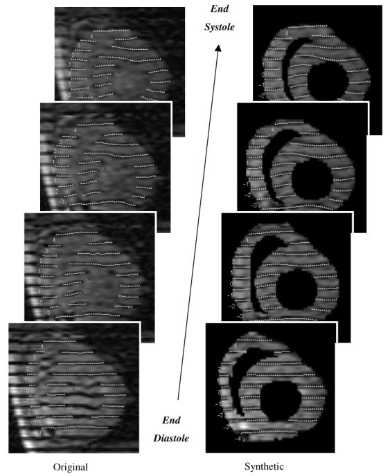
Comparison of images with original tags (left) and masked images with calculated tag lines (right) at different phases of systole.

Figure 13.

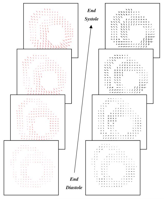
For the same image planes as figure 12, the time evolution of 3D inverse displacement vectors (left column). The maximum and minimum principle strains (right) are displayed on the same homogeneous cardiac grid points. the lines are corresponding respectively to the main stretch and shortening directions (eigenvectors), the length of the lines is proportional to their corresponding eigenvalues.

5. Discussion

The low residual errors indicate that our B-spline based method is successful in capturing the underlying motion of the tissue. The residual errors decrease with increasing control points for all fields, but trying to decrease the error by constantly increasing the parameters is not a realistic approach, as shown here by the validation results. Only when a motion field derived from one set is tested on the points of the other set can its true performance be assessed.

The complexity of the calculation is proportional to the number of control points. Using more control points increases the computational time, but this increase does not necessarily result in a better description of the deformation. As the control point density increases, the deformation field might actually deteriorate for the whole plane, a situation which might not be apparent if one uses only the residual error of current sample points as the only measure.

For inverse field fitting, we have found an adequate control point density for SA image sets to be 8 by 8 in our region of interest (corresponding roughly to an area of 120 by 120 mm). The 8 by 8 control points correspond to about half the tag plane sampling density. The method gets the through-plane information from radially arranged LA images. In one of the related earlier studies (Amini et al 1998), the control points are tied to tag locations, which requires more control points to describe the motion. That approach requires not only that the LA images be a parallel stack but their location must correspond at exact tag locations of the SA images. Since our parametric fields are defined on the imaging planes irrespective to the tag locations we can easily accommodate images with a variable spaced tag pattern (McVeigh and Bolster 1998) or any LA image prescriptions. Radial set LA images are more appropriate for visualization. On the other hand, a disadvantage of our method is the requirement of least-squares based calculation of control points after separate tag segmentation.

We found that a 6×6×6×7 control point density is adequate for forward tracking of cardiac material points (cardiac volume of interest size was 120 by 120 by 100 mm). A fixed inverse control point density (8 × 8) was used when evaluating the forward field. The computational complexity of heart motion tracking depends on the representation. Our compact solution with 6 × 6 × 6 × 7 control points uses cubic B-splines in each direction, both for space or time. For any point, at most four control points at each tensor dimension contribute to the final value.

In this paper, we have validated our motion tracking algorithm for the left ventricle of a normal healthy volunteer. We expect it to perform equally well in cases where the global mechanical activity of the heart is either increased or decreased. For further details on the comparative performance of our method, the reader is referred to another paper in this issue (Declerck 2000). There, we applied our technique to a variety of human and canine hearts as part of a study comparing different cardiac motion analysis techniques. Our technique displayed a nice balance of noise robustness and spatial resolution.

As far as we know, the calculated validation errors of the forward field provide the first in vivo validation of any cardiac motion-tracking algorithm. Although several studies have been done using simulated fields and gel phantoms (Denney and McVeigh 1997, Amini et al 1998), we favour in vivo testing over phantoms or simulated fields because of the intrinsic complexity of the cardiac motion. Our multiple tagging set approach provides a good framework for validating the accuracy of motion tracking algorithms with the confounding factors of in vivo MR imaging, e.g. small breath-holding differences, image artefacts, etc. In the closest example that employed multiple tag orientations on the same heart, Denney and McVeigh (1997) explored the in vivo spatial resolution of their algorithm in a canine heart with high-resolution tags (two 5 mm tag spaced datasets with 2.5 mm offset, giving an effective 2.5 mm tag spacing) and different tag orientations (0, 45, 90 and 135 degrees). They described a method of creating additional displacement fields on material points at the end-systole, creating artificial tag lines and measuring the per cent magnitude response of the reconstructed field by the magnitude of the original field. Their method is helpful in choosing an appropriate distance between tags or deciding between additional tag orientation or tag offsets, but does not quantify the expected errors of the motion tracking method in the in vivo setting. From the validation error results, we determined that our forward motion tracking algorithm produces on average less than a pixel (<1.25 mm) error at end systole for the chosen imaging and tagging parameters.

One of the main obstacles preventing routine clinical use of this type of analysis is the initial contouring of the heart. This is the most time-consuming part of our analysis. Currently it takes around 2 h to contour a complete data set. Although we are working on methods for speeding up the interactive contouring (Shechter et al 1999), a fully automatic cardiac tissue segmentation must be the ultimate goal. Several methods have been proposed in the past, but they require better contrast than the usual image quality we get with cine SPGR images. With methods promising an improvement in the contrast between blood and tissue, as well as an increase of the tag persistence, these problems will be resolved in the near future. At that time, the functional parametric images could be displayed next to the raw MR image while the patient is still in the scanner.

6. Summary

We have presented a stepwise method to achieve a motion field of the heart for tagged MRI images. The advantages of the algorithm described in this paper are: (a) it uses the information from all available tag data; (b) it has a compact parametric representation, so calculations of displacements and material tracking of any point can be done easily; (c) calculated deformation values are continuous both in time and space, as would be natural for the heart tissue; (d) it does not use a chamber specific coordinate system or depend on a specific geometric heart model; (e) it is fast (10 min currently on a desktop PC). Most of the calculations can be run in parallel with a possibility of further increase of speed if desired.

We are currently working on ways of speeding up the process and extending our analysis to full heart (four chambers) motion fields in pathological and normal cases.

Appendix

The least-squares solution with peripheral conditioning for a SA image plane is given here. For the forward field the same technique was applied in 3D. A 2D B-spline displacement field can be written as:

$$d_{i,j,k}=\sum _u\sum _v{B}_u\left(x\right)B_v\left(y\right)C_{i,j,k,u,v}.$$ (14)

For the cubic case, the following knot sequence K defines k cubic control point locations in one parametric direction:K = {0, 0, 0, 0, u₁ . . . u_n . . . u_k-3, 1, 1, 1, 1} where u_n = n/(k - 2) for 1 < n < k - 3.For a given time, the SA image plane and one of two SA tag stacks, optimum control point values describing the displacement, can be found by a least square minimization of

$$E_{i,j,k}=\sum _l\sum _m\left({\Vert d_{i,j,k,l,m}-\left(\sum _u\sum _v{B}_u\left(x_{i,j,k,l,m}\right)B_v\left(y_{i,j,k,l,m}\right)C_{i,j,k,u,v}\right)\Vert }^2\right).$$ (15)

For a given imaging plane, time frame and tagging direction, equation (15) can be thought of as solving a linear set of equations. In matrix form:

$$d=\mathbf{B}\cdot \mathbf{C}$$ (16)

If n is the number of tag points, d is n by 1, B is an n by (k_x*k_y) and C is a (k_x*k_y) by 1 matrix. There are known difficulties of directly inverting B. It is usually ill-conditioned, because of missing data at the periphery of our region of interest (ROI). One attractive solution is to put additional constraints on C values, or regularization (Bajcsy and Kavacis 1989). We have chosen here a different approach: namely, expanding the ROI and providing additional displacement values at the periphery. If done carefully, the piecewise polynomial property of B-splines provides a smooth transition from values at the periphery to the known values at the pericardium. This conditioning process involves the following steps: (a) expand the ROI by an offset (pinning distance) in all directions around the data ranges; (b) overlay a homogeneous grid of points on the expanded ROI; (c) reject all the grid points that are closer to the original points less than a certain threshold (rejection distance); (d) incorporate the remaining grid points into equation (16) with displacement values assigned from the closest original data points. This process essentially tries to minimize the first derivative of the displacement at the periphery. All three parameters involved in this peripheral conditioning process (pinning distance, grid density and rejection distance) are determined empirically: pinning distance is chosen as the tag spacing, a 2D grid with double of the control point density is used, and as a rejection criterion ‘less than half tag spacing’ is employed. Ozturk and McVeigh (1999) employed a similar method but the displacement values at the periphery were set to zero. That approach required a larger pinning distance to operate effectively. We have evaluated the sensitivity of the field fit for these three parameters and observed that within a certain range they did not affect the residual error significantly. Since each basis function has a limited range of support, B in equation (16) is extremely sparce. After conditioning we solve equation (16) directly using fast inversion methods for sparce matrices (Press et al 1988).

References

- Amini AA, Chen Y, Curwen RW, Mani V, Sun J. Coupled B-snake grids and constrained thin-plate splines for analysis of 2-D tissue deformations from tagged MRI. IEEE Trans. Med. Imaging. 1998;17:344–56. doi: 10.1109/42.712124. [DOI] [PubMed] [Google Scholar]
- Axel L, Dougherty L. MR Imaging of motion with spatial modulation of magnetization. Radiology. 1989;171:841–5. doi: 10.1148/radiology.171.3.2717762. [DOI] [PubMed] [Google Scholar]
- Bajcsy R, Kavacis S. Multiresolution elastic matching. Comput. Vision, Graphics Image Process. 1989;46:1–21. [Google Scholar]
- Daniel M. Data fitting with B-spline curves. In: Teixeira JC, Rix J, editors. Modelling and Graphics in Science and Technology. Springer; Berlin: 1996. [Google Scholar]
- deBoor C. A Practical Guide to Splines. Springer; Berlin: 1978. [Google Scholar]
- Declerck J, Denney TS, Ozturk C, O’Dell W, McVeigh ER. Left ventricular motion reconstruction from planar tagged MR images: a comparison. Phys. Med. Biol. 2000;45:1611–32. doi: 10.1088/0031-9155/45/6/315. [DOI] [PMC free article] [PubMed] [Google Scholar]
- Declerck J, Nicholas A, McVeigh ER. Use of a 4D planispheric transformation for the tracking and the analysis of LV motion with tagged MR images. Proc. SPIE. 1999;3660:69–80. [Google Scholar]
- Denney TS, McVeigh ER. Model-free reconstruction of three-dimensional myocardial strain from planar tagged MR images. J. Magn. Reson. Imaging. 1997;7:799–810. doi: 10.1002/jmri.1880070506. [DOI] [PMC free article] [PubMed] [Google Scholar]
- Farin G. Curves and Surfaces for Computer Aided Geometric Design: A Practical Guide. Academic; New York: 1990. [Google Scholar]
- Guttman MA, Prince JL, McVeigh ER. Tag and contour detection in tagged MR images of the left ventricle. IEEE Trans. Med. Imaging. 1994;13:74–88. doi: 10.1109/42.276146. [DOI] [PubMed] [Google Scholar]
- Guttman MA, Zerhouni EA, McVeigh ER. Analysis of cardiac function from MR images. IEEE Comput. Graphics Appl. 1997;17:30–8. doi: 10.1109/38.576854. [DOI] [PMC free article] [PubMed] [Google Scholar]
- McVeigh E. Regional myocardial function. Cardiac Magn. Reson. Imaging. 1998;16:189–206. doi: 10.1016/s0733-8651(05)70008-4. [DOI] [PubMed] [Google Scholar]
- McVeigh ER, Atalar E. Cardiac tagging with breath-hold cine MRI. Magn. Reson. Med. 1992;28:318–27. doi: 10.1002/mrm.1910280214. [DOI] [PMC free article] [PubMed] [Google Scholar]
- McVeigh ER, Bolster BD., Jr Improved sampling of myocardial motion with variable separation tagging. Magn. Reson. Med. 1998;39:657–61. doi: 10.1002/mrm.1910390421. [DOI] [PubMed] [Google Scholar]
- Mosher TJ, Smith MB. A DANTE tagging sequence for the evaluation of translational sample motion. Magn. Reson. Med. 1990;15:334–9. doi: 10.1002/mrm.1910150215. [DOI] [PubMed] [Google Scholar]
- Moulton MJ, Creswell LL, Downing SW, et al. Spline surface interpolation for calculating three-dimensional ventricular strains from MRI tissue tagging. Am. J. Physiol. 1996;270:H281–H297. doi: 10.1152/ajpheart.1996.270.1.H281. [DOI] [PubMed] [Google Scholar]
- O’Dell WG, Moore CC, Hunter WC, Zerhouni EA, McVeigh ER. Displacement field fitting for calculating 3D myocardial deformations from planar tagged MR images. Radiology. 1995;195:829–35. doi: 10.1148/radiology.195.3.7754016. [DOI] [PMC free article] [PubMed] [Google Scholar]
- Ozturk C, McVeigh ER. Four dimensional B-spline based motion analysis of tagged cardiac MR images. Proc. SPIE. 1999;3660:45–56. doi: 10.1088/0031-9155/45/6/319. [DOI] [PMC free article] [PubMed] [Google Scholar]
- Press WH, Flannery BP, Teukolsky SA, Vetterling WT. Numerical Recipes in C. Cambridge University Press; Cambridge: 1988. [Google Scholar]
- Radeva P, Amini AA, Huang J. Deformable B-solids and implicit snakes for 3D localization and tracking of SPAMM MRI data. Comput. Vision Image Understanding. 1997;66:163–78. [Google Scholar]
- Shechter G, Declerck J, Ozturk C, McVeigh ER. Fast template based segmentation of cine cardiac MR. Proc. Int. Soc. Magn. Reson. Med. 1999;7:480. [Google Scholar]
- Spencer AJM. Continuum Mechanics. Longman; London: 1980. [Google Scholar]
- Young AA, Axel L. Three-dimensional motion and deformation of the heart wall: estimation with spatial modulation of magnetization—a model based approach. Radiology. 1995;195:829–35. doi: 10.1148/radiology.185.1.1523316. [DOI] [PubMed] [Google Scholar]
- Young AA, Kraitchman DL, Dougherty L, Axel L. Tracking and finite element analysis of stripe deformation in magnetic resonance tagging. IEEE Trans. Med. Imaging. 1995;14:413–21. doi: 10.1109/42.414605. [DOI] [PubMed] [Google Scholar]
- Zerhouni E, Parish D, Rogers W, Yang A, Shapiro E. Human heart: tagging with MR imaging—a method for noninvasive assessment of myocardial motion. Radiology. 1988;169:59–63. doi: 10.1148/radiology.169.1.3420283. [DOI] [PubMed] [Google Scholar]