Robust Non-Rigid Registration to Capture Brain Shift from Intra-Operative MRI

Abstract

We present a new algorithm to register 3D pre-operative Magnetic Resonance (MR) images to intra-operative MR images of the brain which have undergone brain shift. This algorithm relies on a robust estimation of the deformation from a sparse noisy set of measured displacements. We propose a new framework to compute the displacement field in an iterative process, allowing the solution to gradually move from an approximation formulation (minimizing the sum of a regularization term and a data error term) to an interpolation formulation (least square minimization of the data error term). An outlier rejection step is introduced in this gradual registration process using a weighted least trimmed squares approach, aiming at improving the robustness of the algorithm. We use a patient-specific model discretized with the finite element method (FEM) in order to ensure a realistic mechanical behavior of the brain tissue.

To meet the clinical time constraint, we parallelized the slowest step of the algorithm so that we can perform a full 3D image registration in 35 seconds (including the image update time) on a heterogeneous cluster of 15 PCs. The algorithm has been tested on six cases of brain tumor resection, presenting a brain shift of up to 14 mm. The results show a good ability to recover large displacements, and a limited decrease of accuracy near the tumor resection cavity.

I. Introduction

A. Image-Guided Neurosurgery

The development of intra-operative imaging systems has contributed to improving the course of intra-cranial neurosurgical procedures. Among these systems, the 0.5T intra-operative magnetic resonance scanner of the Brigham and Women’s Hospital (Signa SP, GE Medical Systems, Figure 1) offers the possibility to acquire 256 × 256 × 58 (0.86 mm, 0.86 mm, 2.5 mm) T1 weighted images with the fast spin echo protocol (TR = 400, TE = 16 ms, FOV = 220x220 mm) in 3 minutes and 40 seconds. The quality of every 256 × 256 slice acquired intra-operatively is fairly similar to images acquired with a 1.5T conventional scanner, but the major drawback of the intra-operative image remains the slice thickness (2.5 mm). Images do not show significant distortion, but can suffer from artifacts due to different factors (surgical instruments, hand movement, radio-frequency noise from bipolar coagulation). Recent advances in acquisition protocol [1] however make it possible to acquire images with very limited artifacts during the course of a neurosurgical procedure.

Fig. 1.

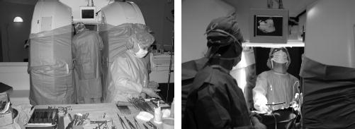
The 0.5 T open magnet system (Signa SP, GE Medical Systems) of the Brigham and Women’s Hospital

The intra-operative MR scanner enhances the surgeon’s view and enables the visualization of the brain deformation during the procedure [2], [3]. This deformation is a consequence of various combined factors: cerebro spinal fluid (CSF) leakage, gravity, edema, tumor mass effect, brain parenchyma resection or retraction, and administration of osmotic diuretics [4]–[6]. Intra-operative measurements show that this deformation is an important source of error that needs to be considered [7]. Indeed, imaging the brain during the procedure makes the tumor resection more effective [8], and facilitates complete resections in critical brain areas. However, even if the intra-operative MR scanner provides significantly more information than any other intra-operative imaging system, it is not clinically possible to acquire image modalities like diffusion tensor MR, functional MR or high resolution MR images in a reasonable time during the procedure. Illustrated examples of image guided neurosurgical procedures can be found on the SPL web-site.¹

Non-rigid registration algorithms provide a way to overcome the intra-operative acquisition problem: instead of time-consuming image acquisitions during the procedure, the intra-operative deformation is measured on fast acquisitions of intra-operative images. This transformation is then used to match the pre-operative images on the intra-operative data. To be used in a clinical environment, the registration algorithm must hence satisfy different constraints:

• Speed. The registration process should be sufficiently fast such that it does not compromise the workflow during the surgery. For example, a process time less than or equal to the intra-operative acquisition time is satisfactory.

• Robustness. The registration results should not be altered by image intensity inhomogeneities, artifacts, or by the presence of resection in the intra-operative image.

• Accuracy. The registration displacement field should reflect the physical deformation of the underlying organ.

The choice of the number and frequency of image acquisitions during the procedure remains an open problem. Indeed, there is a trade-off between acquiring more images for accurate guidance and not increasing the time for imaging. The optimal number of imaging sessions may depend on the procedure type, physiological parameters and the current amount of deformation. Other imaging devices (stereo-vision, laser range scanner, ultrasound...) could be additionally used to assist the surgeon in his decision. Those perspectives are currently under investigation in our group [9].

In this paper, we introduce a new registration algorithm designed for image-guided neurosurgery. We rely on a biomechanical finite element model to enforce a realistic deformation of the brain. With this physics-based approach, apriori knowledge in the relative stiffness of the intra-cranial structures (brain parenchyma, ventricles...) can be introduced.

The algorithm relies on a sparse displacement field estimated with a block matching approach. We propose to compute the deformation from these displacements using an iterative method that gradually shift from an approximation problem (minimizing the sum of a regularization term and a data error term) towards an interpolation problem (least square minimization of the data error term). To our knowledge, this is the first attempt to take advantage of the two classical formulations of the registration problem (approximation and interpolation) to increase both robustness and accuracy of the algorithm.

In addition, we address the problem of information distribution in the images (known as the aperture problem [10] in computer vision) to make the registration process depend on the spatial distribution of the information given by the structure tensor (see Section II-A.5 for definition).

We tested our algorithm on six cases of brain tumor resection performed at Brigham and Women’s hospital using the 0.5 T open magnet system. The pre-operative images were usually acquired the day before the surgery. The intra-operative dataset is composed of six anatomical 256 × 256 × 58 T1 weighted MR images acquired with the fast spin echo protocol previously described. Usually, an initial intra-operative MR image is acquired at the very beginning of the procedure, before opening of the dura-mater. This image, which does not yet show any deformation, is used to compute the rigid transformation between the two positions of the patient in any pre-operative image and the image from the intra-operative scanner.

B. Non-Rigid Registration for Image-Guided Surgery

1) Modeling the Intra-Operative Deformation: Because of the lower resolution of the intra-operative imaging devices, modeling the behavior of the brain remains a key issue to introduce a priori knowledge in the image-guided surgery process. The rheological experiments of Miller significantly contributed in the understanding of the physics of the brain tissue [11]. His extensive investigation in brain tissue engineering showed very good concordance of the hyper-viscoelastic constitutive equation with in vivo and in vitro experiments. Miga et al. demonstrated that a patient-specific model can accurately simulate both the intra-operative gravity and resection-induced brain deformation [12], [13]. A practical difficulty associated with these models is the extensive time necessary to mesh the brain and solve the problem. Castellano-Smith et al. [14] addressed the meshing time problem by warping a template mesh to the patient geometry. Davatzikos et al. [15] proposed a statistical framework consisting of pre-computing the main mode of deformation of the brain using a biomechanical model. Recent extensions of this framework showed promising results for intra-operative surgical guidance based on sparse data [16].

2) Displacement-Based Non-Rigid Registration: In this paper, we propose a displacement-based non-rigid registration method consisting in optimizing a parametric transformation from a sparse set of estimated displacements.

Alternative methods include intensity-based methods where the parametric transformation is estimated by minimizing a global voxel-based functional defined on the whole image. It should be noted that although these algorithms are by nature computationally expensive, the work of Hastreiter et al. [17] based on an openGL acceleration, or the work of Rohlfing et al. [18] using shared-memory multiprocessor environments to speed up the free form deformation-based registration [19] recently demonstrated that such algorithms could be adapted to the intra-operative registration problem.

The following review of the literature is purposely restricted to registration algorithms based on approximation and interpolation problems in the context of matching corresponding points using an elastic model constraint.

a) Interpolation: Simple biomechanical models have been used to interpolate the full brain deformation based on sparse measured displacements. Audette [20] and Miga et al. [21] measured the visible intra-operative cortex shift using a laser range scanner. The displacement of deep brain structures was then obtained by applying these displacements as boundary conditions to the brain mesh. A similar surface based approach was proposed by Skrinjar et al. [22] and Sun et al. [23] imaging the brain surface with a stereo vision system. Ferrant et al. [24] extracted the full cortex and ventricles surfaces from intra-operative MR images to constrain the displacement of the surface of a linear finite element model. These surface-based methods showed very good accuracy near the boundary conditions, but suffered from as lack of data inside the brain [6]. Rexilius et al. [25] followed Ferrant’s efforts by incorporating block-matching estimated displacements as internal boundary condition to the FEM model (leading to the solution presented in Section II-C.2). However the method proposed by Rexilius was not robust to outliers. Ruiz-Alzola et al. [26] proposed through the Kriging interpolator a probabilistic framework to manage the noise distribution in the sparse displacement field computed with the block matching algorithm. Although first results show qualitative good matching, it is difficult to assess the realism of the deformation since the Kriging estimator does not rely on a physical model.

b) Approximation: The approximation-based registration consists in formulating the problem as a functional minimization decomposed into a similarity energy and a regularization energy. Because its formulation leads to well posed problems, the similarity energy often relies on a block (or feature) matching algorithm. In 1998, Yeung et al. [27] showed impressive registration results on a phantom using an approximation formulation combining ultrasound speckle tracking with a mechanical finite element model. Hata et al. [28] registered pre-operative with intra-operative MR images using a mutual information based similarity criterion (see Wells et al. paper for details about mutual information [29]) and a mechanical finite element model to get plausible displacements. He could perform a full image registration using a stochastic gradient descent search in less than 10 minutes, for an average error of 40% of true displacement. Rohr et al. [30] improved the basic block matching algorithm by selecting relevant anatomical landmarks in the image and taking into account the anisotropic matching error in the global functional. Shen et al. [31] investigated this idea of anatomical landmarks and proposed an attribute vector for each voxel reflecting the underlying anatomy at different scales. In addition to the Laplacian smoothness energy, their energy minimization involves two different data similarity functions for pushing and pulling the displacement to the minimum of the functional energy.

II. Method

We have developed a registration algorithm to measure the brain deformation based on two images acquired before and during the surgery. The algorithm can be decomposed into three main parts, presented in Figure 2. The first part consists in building a patient specific model corresponding to the patient position in the open-magnet scanner. Patient-specific in this algorithm’s context refers to having a coarse finite element model that approximately matches the outer curvature of the patient’s cortical surface and lateral ventricular surfaces. The second part is the block matching computation for selected blocks. The third part is the iterative hybrid solver from approximation to interpolation.

Fig. 2.

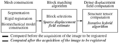
Overview of the steps involved in the registration process.

As suggested in Figure 2, a large part of the computation can be done before acquiring the intra-operative MR image. In the following section, we propose a description of the algorithm sequence, making a distinction between pre-operative and intra-operative computations. Indeed, since the pre-operative image is available hours before surgery, we can use preprocessing algorithms to:

• segment the brain, the ventricles and the tumor.

• Build the patient-specific biomechanical model of the brain based on the previous segmentation.

• Select blocks in the pre-operative image with relevant information.

• Compute the structure tensor in the selected blocks.

Note that the rigid registration between the pre-operative image and the intra-operative image is computed before the acquisition of the image to be registered, after the beginning of the procedure. Indeed, the rigid motion between the two positions of the patient is estimated on the first intra-operative image acquired at the very beginning of the surgical procedure, before opening the skull and the dura.

After the first intra-operative acquisition showing deformations, it is important to minimize the computation time. As soon as this image is acquired, we compute for each selected block in the pre-operative image the displacement that minimizes a similarity measure. We chose the coefficient of correlation as the similarity measure, also providing a confidence in the measured displacement for every block.

The registration problem, combining a finite element model with a sparse displacement field, can then be posed in terms of approximation and interpolation. The two formulations however come with weaknesses, further detailed in Section II-C.1. We thus propose a new gradual hybrid approach from the approximation to the interpolation problem, coupled with an outlier rejection algorithm to take advantage of both classical formulations.

A. Pre-Operative MR Image Treatment

1) Segmentation: We use the method proposed by Mangin et al. [32] and implemented in Brainvisa² to segment the brain in the pre-operative images (see Figure 3). The tumor segmentation is extracted from the pre-operative manual delineation created by the physician for the pre-operative planning.

Fig. 3.

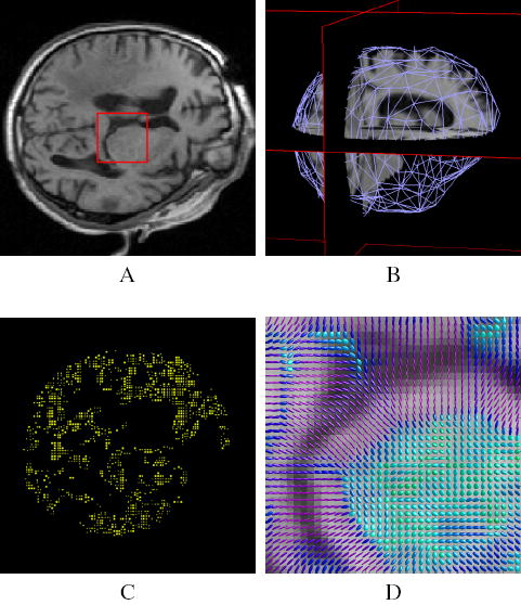
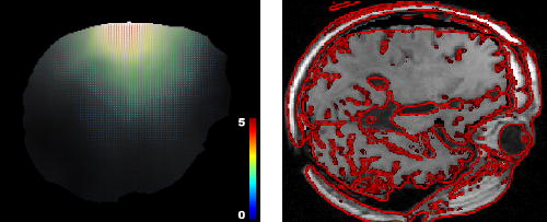
Illustration of the pre-operative processes. (A) pre-operative image. (B) segmentation of the brain and 3D mesh generation (we only represent the surface mesh for visualization convenience). (C) Example of block selection, choosing 5% of the total brain voxels as blocks centers. Only the central voxel of the selected blocks is displayed. (D) Structure tensor visualization as ellipsoids (zoom on the red square), the color of the tensors demonstrates the fractional anisotropy.

2) Rigid Registration: We match our initial segmentation to the first intra-operative image (actually acquired before the dura mater opening) using the rigid registration software developed at INRIA by Ourselin et al. [33], [34]. This software, also relying on block matching, computes the rigid motion that minimizes the transformation error with respect to the measured displacements. Detailed accuracy and robustness measures can be found in [35].

3) Biomechanical Model: The full meshing procedure is decomposed into three steps: we generate a triangular surface mesh from the brain segmentation with the marching cubes algorithm [36]. This surface mesh is then decimated with the YAMS software (INRIA) [37]. The volumetric tetrahedral mesh is finally built from the triangular one with another INRIA software: GHS3D [38]. This software optimizes the shape quality of all tetrahedra in the final mesh.

The mesh generated has an average number of 10,000 tetra-hedra (about 1700 vertices), which proved to be a reasonable trade-off between the number of degrees of freedom and the number of matches (about 1 to 15, see Section II-C.2 for a discussion about the influence of this ratio).

We rely on the finite element theory (see [39] for a complete review of the finite element formalism) and consider an incompressible linear elastic constitutive equation to characterize the mechanical behavior of the brain parenchyma. Choosing the Young modulus for the brain tissue E = 694Pa and assuming slow and small deformations (≤ 10%), we have shown that the maximum error measured on the Young modulus with respect to the state of the art brain constitutive equation [11] is less than 7% [40]. We chose a Poisson’s ratio ν = 0.45, modeling an almost incompressible brain tissue. Because the ventricles and the subarachnoid space are connected to each other, the CSF is free to flow between them. We thus assume very soft and compressible tissue for the ventricles (E = 10Pa and ν = 0.05).

4) Block Selection: The relevance of a displacement estimated with a block matching algorithm depends on the existence of highly discriminant structures in this block. Indeed, an homogeneous block lying in the white matter of the pre-operative image might be similar to many blocks in the intra-operative image, so that its discriminant ability is lower than a block centered on a sulcus. We use the block variance to measure its relevance and only select a fraction of all potential blocks based on this criterion (an example of 5% block selection is given in Figure 3).

The drawback of this method is a selection of blocks in clusters where overlapping blocks share most of their voxels. We thus introduce the notion of prohibited connectivity between two block centers to prevent two selected blocks to be too close to each other. We implemented a variety of connectivity criteria, and obtained best results using the 26 connectivity (with respect to the central voxel), preventing two distinct blocks of 7 × 7 × 7 voxels to share more than 42% overlapping voxels. Note that this prohibited connectivity criterion leads to a maximum of 30,000 blocks selected in an average adult brain (≈ 1300 cm³) imaged with a resolution of 0.86 mm × 0.86 mm × 2.5 mm. Note also that the 7 × 7 × 7 blocks used in this paper are about three times longer in the Z direction because of the anisotropic voxel size.

In addition, to anticipate the ill-posed nature of finding correspondences in the tumor resection cavity, we performed the block selection inside a mask corresponding to the brain without the tumor.

5) Computation of the Structure Tensor: It has been proposed in the literature to use the information distribution around a voxel as a mean of selecting blocks [26] or as an attribute considered for the matching of two voxels [31]. Recent works assess the problem of ambiguity raised by the anisotropic character of the intensity distribution around a voxel in landmark matching-based algorithms: edges and lines lead respectively to first and second order ambiguities, meaning that a block correlation method can only recover displacements in their orthogonal directions. Rohr et al. account for this ambiguity by weighting the error functional related to each landmark displacement with a covariance matrix [30].

In this paper, we consider the normalized structure tensor Tk defined in the pre-operative iamge I at position O_k by:

$$T_k=\frac{G\ast (\nabla I(O_k)){(\nabla I(O_k))}^T}{\mathit{trace}\hspace{0.17em}[G\ast (\nabla I(O_k)){(\nabla I(O_k))}^T]}$$ (1)

∇I(O_k) is the Sobel gradient computed at voxel position Ok, and G defines a convolution kernel. A Gaussian kernel is usually chosen to compute the structure tensor. In our case, since all voxels in a block have the same influence, we use a constant convolution kernel G in a block, so that each (∇I(O_k))(∇I(O_k))^T has the same weight in the computation of T_k.

This positive definite second order tensor represents the structure of the edges in the image. If we consider the classical ellipsoid representation, the more the underlying image resembles to a sharp edge, the more the tensor elongates in the direction orthogonal to this edge (see image D of Figure 3). The structure tensor provides a three dimensional measure of the smoothness of the intensity distribution in a block and thus a confidence in the measured displacement for this block. In Section II-C, we will see how to introduce this confidence in the registration problem formulation.

B. Block Matching Algorithm

Also known as template or window matching, the block matching algorithm is a simple method used for decades in computer vision [41], [42]. It makes the assumption that a global deformation results in translation for small parts of the image. Then the global complex optimization problem can be decomposed into many simple ones: considering a block B(O_k) in the reference image centered in O_k, and a similarity metric between two blocks M(B(O_a), B(O_b)), the block matching algorithm consists in finding the positions O′_k that maximize the similarity:

$$arg\hspace{0.17em}\underset{O^{\prime }}{max}\hspace{0.17em}[M\hspace{0.17em}(B(O_k),\hspace{0.17em}B({O^{\prime }}_k))]$$ (2)

Performing this operation on every selected block in the pre-operative image produces a sparse estimation of the displacement between the two images (see Figure 4). In our algorithm, the block-matching is an exhaustive search performed once, and limited to integral voxel translation. It is limited to the brain segmentation, thus restricting the displacements to the intra-cranial region.

Fig. 4.

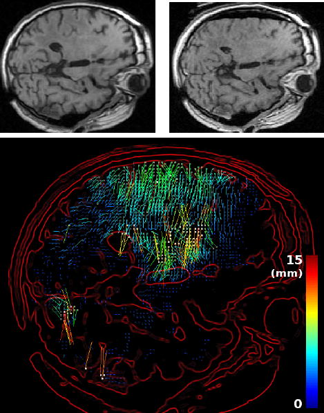
Block matching-based displacements estimation. Top left: slice of the pre-operative MR image. Top right: intra-operative MR image. Bottom: the sparse displacement field estimated with the block matching algorithm and superposed to the gradient of the pre-operative image (5% block selection, using the coefficient of correlation). The color scale encodes the norm of the displacement, in millimeters.

The choice of the similarity function has largely been debated in the literature, we will refer the reader to the article of Roche et al. [43] for a detailed comparison of them. In our case, the mono-modal (MR-T1 weighted) nature of the registration problem allows us to make the strong assumption of an affine relationship between the two image intensity distributions. The correlation coefficient thus appears as a natural choice adapted to our problem:

$$c=\frac{{\sum }_{X\in B}(B_F(X)-{\overline{B}}_F)(B_T(X)-{\overline{B}}_T)}{{\sum }_{X\in B}{B}_F(X)B_T(X)-{\overline{B}}_F{\overline{B}}_T}$$ (3)

Where B_F and B_T denote respectively for the block in the floating and in the reference image, and $\overline{B}$ for the average intensity in block B. In addition, the value of the correlation coefficient for two matching blocks is normalized between 0 and 1 and reflects the quality of the matching: a value close to 1 indicates two blocks very similar while a value close to 0 for two blocks very different. We use this value as a confidence in the displacement measured by the block matching algorithm.

C. Formulation of the Problem: Approximation Versus Interpolation

As we have seen in Section I-B, the registration problem can be either formulated as an approximation, or as an interpolation problem. In this section, we will show how to formulate our problem in both terms and describe the associated advantages and disadvantages.

1) Approximation: The approximation problem can be formulated as an energy minimization. This energy is composed of a mechanical and a matching (or error) energy:

with:

• U the mesh displacement vector, of size 3n, with n number of vertices.

• K the mesh stiffness matrix of size 3n × 3n. Details about the building of the stiffness matrix can be found in [44].

• H is the linear interpolation matrix of size 3p × 3n. One mesh vertex v_i, i ∈ [1:n] corresponds to three columns of H (columns [3 *i+ 1 : 3 *i+ 3]). One matching point k (ie one block center O_k) corresponds to three rows of H (rows [3 * k + 1 : 3 * k + 3]). The 3 × 3 sub-matrices [H]_ki are defined as: [H]_kcj = diag(h_j, h_j, h_j) for the four columns c_j, j∈[1 : 4] corresponding to the four points v_cj of the tetrahedron containing the center of the block O_k, and [H]_ki = 0 everywhere else. The linear interpolation factor h_j, j ∈ [1:4] are computed for the block center O_k inside the tetrahedron with:

$$\left[\begin{array}{c}{h}_1\\ h_2\\ h_3\\ h_4\end{array}\right]={\left[\begin{array}{cccc}{v}_{c_1}^x& v_{c_2}^x& v_{c_3}^x& v_{c_4}^x\\ v_{c_1}^y& v_{c_2}^y& v_{c_3}^y& v_{c_4}^y\\ v_{c_1}^z& v_{c_2}^z& v_{c_3}^z& v_{c_4}^z\\ 1& 1& 1& 1\end{array}\right]}^{-1}\left[\begin{array}{c}{O_k}^x\\ {O_k}^y\\ {O_k}^z\\ 1\end{array}\right]$$ (5)

• D the block-matching computed displacement vector of size 3p, with p number of matched points. Note that HU - D defines the error on estimated displacements.

• S the matching stiffness of size 3p × 3p.

Usually, a diagonal matrix is considered in the matching energy aiming at minimizing the sum of squared errors. In our case, this would lead to $S=\frac{\alpha }{p}I$defines the identity matrix, α defines the trade-off between the mechanical energy and the matching energy, it can also be interpreted as the stiffness of a spring toward each block matching target (the unit of α is N.m⁻¹). The $\frac{1}{p}$ factor is used to make the global matching energy independent of the number of selected blocks.

We propose an extension to the classical diagonal stiffness matrix S case, taking into account the matching confidence from the correlation coefficient (Equation 3) and the local structure distribution from the structure tensor (Equation 1) in the matching stiffness. These measures are introduced through the matrix S, which becomes a block-diagonal matrix whose 3 × 3 sub-matrices S_k are defined for each block k as:

$$S_k=\frac{\alpha }{p}{c}_k{T}_k$$ (6)

The influence of a block thus depends on two factors:

• the value of the coefficient of correlation: the better the correlation is (coefficient of correlation closer to 1), then the higher the influence of the block on the registration will be.

• The direction of matching with respect to the tensor of structure: we only consider the matching direction co-linear to the orientation of the intensity gradient in the block.

The minimization of Equation 4 is classically obtained by solving $\frac{\partial W}{\partial U}=0$:

$$\frac{\partial W}{\partial U}=[K+H^{T}SH]U-H^{T}SD=0$$ (7)

Leading to the linear system:

$$[K+H^{T}SH]U=H^{T}SD$$ (8)

Solving Equation 8 for U leads to the solution of the approximation problem. As shown on Figure 5, the main advantage of this formulation lies in its ability to smooth the initial displacement field using strong mechanical assumptions. The approximation formulation however suffers from a systematic error: whatever the value chosen for E and α, the final displacement of the brain mesh is a trade-off between the pre-operative rest position and the measured positions so that the deformed structures never reach the measured displacements (visible on Figure 5 for the ventricles and cortical displacement).

Fig. 5.

Solving the registration problem using the approximation formulation (shown on the same slice as Figure 4). Left: dense displacement computed as the solution of Equation 8. Right: gradient of the target image superimposed on the pre-operative deformed image using the computed displacement field. We can observe a systematic error on large displacements.

2) Interpolation: The interpolation formulation consists in finding the optimal mesh displacements U that minimize the data error criterion:

$$arg\hspace{0.17em}\underset{U}{min}\hspace{0.17em}{(HU-D)}^T(HU-D)$$ (9)

The vertex displacement vector U satisfying Equation 9 is then given by:

$$U={(H^{T}H)}^{-1}{H}^{T}D$$ (10)

In this paper, the possible values for D are restricted to integral voxel translations. However the displacement of a single vertex depends on all the matches included in the surrounding tetrahedra, so that its displacement is a weighted combination of all these matches. The mesh thus also serves the function of regularization on the estimated displacements. Therefore, if the ratio of the number of degrees of freedom (U) to the number of block displacement (D) is small enough (typically < 0.1), sub-voxel accuracy (with respect to the ”true” transformation) can be expected, even with integral displacements. Conversely, if the previous ratio is greater than or close to one, the regularization due to the limited number of degrees of freedom is lost, and the transformation can be discontinuous because of the sampling effect. Using a refined mesh could thus induce an additional displacement error (up to half a voxel size), and makes this method inappropriate to estimate brain tissue stress. The ratio used for this paper is about 15 matches per vertex.

Solving Equation 10 without matches in a vertex cell, lead to an undetermined displacement for this vertex. The sparseness of the estimated displacements could thus prevent some areas of the brain from moving because they are not related to any blocks. One way of assessing this problem is to take into account the mechanical behavior of the tissue. The problem is turned into a mechanical energy minimization under the constraint of minimum data error imposed by Equation 10. The minimization under constraint is formalized through the Lagrange Multipliers stored in a vector $\stackrel{\sim }{F}$:

$$\stackrel{\sim }{W}=U^{T}KU+{\stackrel{\sim }{F}}^T{H}^T(HU-D)$$ (11)

The Lagrange multiplier vector $\stackrel{\sim }{F}$of size 3n can be interpreted as the set of forces applied at each vertex U in order to impose the displacement constraints. Note that the second term ${\stackrel{\sim }{F}}^T{H}^T(HU-D)$ is homogeneous to an elastic energy. Once again, the optimal displacements and forces are obtained by writing that $\frac{\partial \stackrel{\sim }{W}}{\partial U}=0$and $\frac{\partial \stackrel{\sim }{W}}{\partial \stackrel{\sim }{F}}=0.$ One then obtain:

$$KU+H^{T}H\stackrel{\sim }{F}=0$$ (12)

$$H^{T}HU-H^{T}D=0$$ (13)

A classic method is then to solve:

$$\left[\begin{array}{cc}K& H^{T}H\\ H^{T}H& 0\end{array}\right]\left[\begin{array}{c}U\\ \stackrel{\sim }{F}\end{array}\right]=\left[\begin{array}{c}0\\ H^{T}D\end{array}\right]$$ (14)

The main advantage of the interpolation formulation is an optimal displacement field (that minimizes the error) with respect to the matches. However, when matches are noisy or -worse- when some of them are outliers (such as in the region around the tumor on Figure 6), the recovered displacement is disturbed and does not follow the displacement of the tissue. Some of the mesh tetrahedra can even flip, modeling a non dif-feomorphic deformation. This transformation is obviously not physically acceptable, and emphasizes the need for selecting mechanically realistic matches.

Fig. 6.

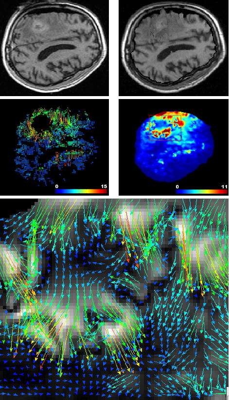
Solving the registration problem using the interpolation formulation leads to poor matches. Top left: intra-operative MR image intersecting the tumor. Top right: result of the registration of the pre-operative on the intra-operative image using the interpolation formulation (Equation 14). Middle left: estimated displacement using the block matching algorithm (same slice). Middle right: norm of the recovered displacement field using the interpolation formulation. Bottom: zoom on the registration displacement field around the tumor region (red box) indicates disturbed displacements.

D. Robust Gradual Transformation Estimate

1) Formulation: We have seen in Section II-C that the approximation formulation performs well in the presence of noise but suffers from a systematic error. Alternatively, solving the exact interpolation problem based on noisy data is not adequate.

We developed an algorithm which takes advantage of both formulations to iteratively estimate the deformation from the approximation to the interpolation based formulation while rejecting outliers. The gradual convergence to the interpolation solution is achieved through the use of an external force F added to the approximation formulation of Equation 8, which balances the internal mesh stress:

$$[K+H^{T}SH]\hspace{0.17em}U=H^{T}SD+F$$ (15)

This force F_i is computed at each iteration i to balance the mesh internal force KU_i. This leads to the iterative scheme:

$$F_i\Leftarrow K{U}_i$$ (16)

$$U_{i+1}\Leftarrow {[K+H^{T}S\hspace{0.17em}H]}^{-1}[H^{T}SD+F_i]$$ (17)

The transformation is then estimated in a coarse to fine approach, from large deformations to small details up to the interpolation. We propose in appendix a proof of convergence of the algorithm toward the interpolation formulation.

This new formulation combines the advantages of robustness to noise at the beginning of the algorithm and accuracy when reaching convergence. Because some of the measured displacements are outliers, we propose to introduce a robust block-rejection step based on a least-trimmed squares algorithm [45]. This algorithm rejects a fraction of the total blocks based on an error function ξ_k measuring for block k the error between the current mesh displacement and the matching target:

$${\xi }_k=\parallel S_k[{(HU)}_k-D_k]\parallel$$ (18)

D_k, (HU)_k and [(HU)_k − D_k] respectively define the measured displacement, the current mesh-induced displacement and the current displacement error for the block k. ξ_k is thus simply the displacement error weighted according to the direction of the intensity gradient in block k. However, our experiments showed that the block matching error is rather multiplicative than additive (i.e. the larger the displacement of the tissue, the larger the measured displacement error). Therefore, we modified ξ to take into account the current estimate of the displacement:

$${\xi }_k=\frac{\parallel S_k[{(HU)}_k-D_k]\parallel }{\lambda \parallel {(HU)}_k\parallel +1}$$ (19)

λ is a parameter of the algorithm tailored to the error distribution on matches. Note that a log-error function could also have been used. With such a cost function, the rejection criterion is more flexible with points that account for larger displacements. The matrices S and H now have to be recomputed at each iteration involving an outlier rejection step.

The number of rejection steps based on this error function, as well as the fraction of blocks rejected per iteration are defined by the user. The algorithm then iterates the numerical scheme defined by Equations 16 and 17 until convergence. Figure 7 gives an example of the registered image and the associated displacement field at convergence. The final registration scheme is given in Algorithm 1.

Fig. 7.

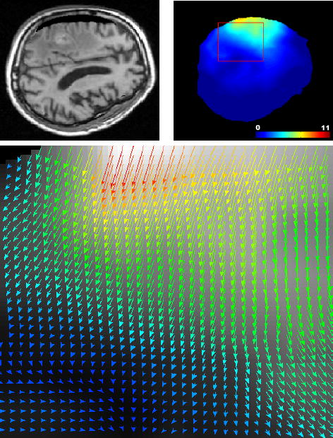
Solving the registration problem using the proposed iterative approach (Algorithm 1). Top left: result of the registration of the pre-operative on the intra-operative image using the iterative formulation (same slice as Figure 6). Top right: norm of the recovered displacement field. Bottom: zoom on the registration displacement field around the tumor region (red box) indicates realistic displacements.

2) Parameter setting: We used 7 ×7 ×7 blocks, searching in a 11 × 11 × 25 window (we used a larger window in the direction of larger displacement: following gravity as observed in [46]) with an integral translation step of 1 × 1 × 1.

Although the least trimmed squares algorithm is a robust estimator up to 50% of outliers [45], we experienced that a cumulated rejection rate representing 25% of the total initial selected blocks is sufficient to reject every significant outlier. Figure 8 shows the evolution in the ouliers rejection scheme. A variation of ± 5% does not have a significant influence on the registration. Below 20%, a quantitative examination of the matches reveals that some outliers could remain. Over 30%, relevant information is discarded in some regions, the displacement then follows the mechanical model in these regions.

Fig. 8.

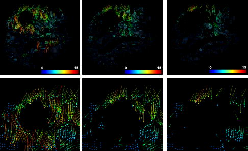
Visualization of the block-rejection step on the same patient as Figure 6 (2.5% of blocks rejected per iteration). Left: initial matches. Middle: after 5 iterations (12.5% rejection). Right: final selected matches after 10 iterations of block rejection (25% of the total blocks are rejected). The region around the tumor seems to have a larger rejection rate than the rest of the brain (especially below the tumor). A closer look at this region (bottom row) reveals that lots of matches around the tumor point toward a wrong direction.

λ defines the breakup point between an additive and a multiplicative error model: with displacements less (respectively more) than $\frac{1}{\lambda }$mm, the model is additive (respectively multiplicative). This value thus has to be adapted to the accuracy of the matches, which is closely related to the noise in images. The value of λ has been estimated empirically: $\frac{1}{2}$ gave best results, but we encountered significant changes (average difference on the displacement of 2 × 10⁻² mm, standard deviation of 4 × 10⁻² mm and maximum displacement difference of 1.1 mm on the dataset) for variations of lambda upto $\pm \frac{1}{10}.$

The last parameter is the matching stiffness a. Even if it does not influence the convergence, its value might indeed disturb the rejection steps if the convergence rate is too slow. The largest displacements could indeed be considered as outliers if the matching energy does not balance fast enough the mechanical one. Therefore we chose a matching stiffness $\alpha =\frac{\mathit{trace}(K)}{n}$, reflecting the average vertex stiffness (note that this value does not depend on the number of vertices used to mesh the volume), so that at least half of the displacement is already recovered after the first iteration. Experiments showed that the results are almost unchanged (max. difference < 0.1 mm) when α is scaled (multiplied of divided) by a factor of 5.

3) Implementation Issues andsTime Constraint: The mechanical system was solved using the conjugate gradient (see [47] for details) method with the GMM++ sparse linear system solver³. The rejected block fraction for 1 iteration was set to 2.5% and the number of rejection steps to 10. The following computation times have been recorded on the first patient of our database, using a Pentium IV 3Ghz machine running the sequential algorithm:

• Block matching computation ↦ 162 sec.

• Building matrices S, H, K and vector D ↦ 1.8 sec.

• Computing external force vector (Equation 16) ↦ 7 × 10⁻² sec/iteration.

• Solve system (Equation 17) ↦ 9 × 10⁻² sec/iteration.

• Blocks rejection ↦ 12 × 10⁻² sec/iteration.

• Update H, S, D ↦ 25 × 10⁻² sec/iteration.

Most of the computation time is spent in the block matching algorithm. We developed a parallel version of it using PVM⁴ able to run on an heterogeneous cluster of PCs, and taking advantage of the sparse computing resource available in a clinical environment. This version reduced the block matching computation time to 25 seconds on an heterogeneous group of 15 PCs, composed of 3 dual Pentium IV 3Ghz, 3 dual Pentium IV 2Ghz and 9 dual Pentium III 1Ghz. Similar hardware is widely available in hospitals and additionally very inexpensive compared to high-performance computers. The full 3D registration process (including the image update time) could thus be achieved in less than 35 seconds, after 15 iterations of the algorithm. We think that this time is compatible with the constraint imposed by the procedure.

III. Experiments

We evaluated our algorithm on 6 pairs of pre and intra-operative MR T1 weighted images. For every patient, the intra-operative registered image is always the last full MR image acquired during the procedure (acquired one to four hours after the opening of the dura). The skin, skull, and dura are opened, and significant brain resection was performed at this time. The 6 experiments have been run using the same set of parameters. Figure 9 presents the 6 pre-operative image registrations compared with the intra-operative images on the slice showing the largest displacement (which does not necessarily show the resection cavity) ⁵. Pre-operative, intra-operative and warped images are shown on corresponding slices after rigid registration.

Fig. 9.

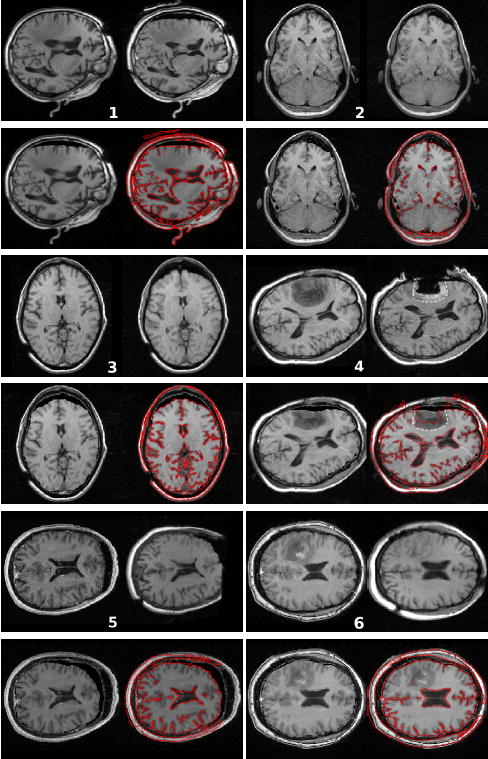
Result of the non-rigid registration of the pre-operative image on the intra-operative image. For each patient: (top left) pre-operative image; (top right) intra-operative image; (bottom left) result of the registration: deformation of the pre-operative image on the intra-operative image; (bottom right) gradient of the intra-operative image superimposed on the result image. The enhanced region on patient’s 4 image indicates that the resection is incomplete. The white dotted line shows where the outline of the tumour is predicted to be after deformation (top right). It shows a reasonable matching with the tumor margin in the deformed image (bottom right).

The registration algorithm shows qualitatively good results: the displacement field is smooth and reflects the tissue behavior, the algorithm can still recover large deformations (up to 14mm for patient 5). We wish also to emphasize the fact that the algorithm does not require manual interaction making it fully automatic following the intra-operative MR scan.

We can observe that the quality of the brain segmentation has a direct influence on the deformed image, for example patient 3 of Figure 9 had a brain mask eroded on the frontal lobe which misses in the registered image. The deformation field however should not suffer from the mask inaccuracy, since the brain segmentation is not directly used to guide the registration. The assumption of local translation in the block-matching algorithm seems to be well adapted to the motion of the brain parenchyma. It shows some limitations for ventricles expansion (patient 4 and 6 of Figure 9) or collapse (patient 5 of Figure 9), where the error is approximately between two and three millimeters.

The accuracy of the algorithm has been quantitatively evaluated by a medical expert selecting corresponding feature points in the registration result image and the target intra-operative image. This landmark-based error (not limited to in-plane error) estimation has been performed on every image for 9 different points. Figure 10 presents the measured error for the 54 landmarks as a function of the displacement of the tissue and Figure 11 presents the measured error for the 54 landmarks as a function of the distance to the tumor. Table I gives the global values of the registration error.

Fig. 10.

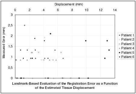
Measure of the registration error for 54 landmarks as a function of the initial error (i.e. as a function of the real displacement of tissue, estimated with the landmarks).

Fig. 11.

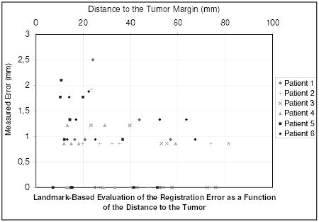
Measure of the registration error for 54 landmarks as a function of the distance to the tumor margin.

TABLE I.

Quantitative assessment of the registration accuracy.

	All patients	Patient 1	Patient 2	Patient 3	Patient 4	Patient 5	Patient 6
Max. displacement (mm)	13.18	6.73	4.10	7.77	5.74	13.18	4.60
Mean displacement ± std. dev. (mm)	3.77±3.3	3.63±2.4	2.41±1.9	2.89±3.0	2.71±1.9	8.06±4.5	2.36±1.3
Mean error ± std. dev. (mm)	0.75±0.6	0.73±0.8	0.69±0.6	0.45±0.5	0.58±0.5	0.88±0.8	1.16±0.5
Max. error (mm)	2.50	2.50	1.92	1.21	1.21	2.10	1.88
Mean relative error (%)	19	20	28	15	21	10	49

The error distribution presented on figure 10 looks un-correlated to the displacement of the tissue. This highlights the potential of this algorithm to recover large displacements. Whereas the error is limited (table I: 0.75 mm in average, 2.5 mm at maximum), Figure 11 shows that the error somewhat increases when getting closer to the tumor. Because a substantial number of matches are rejected as outliers around the tumor, the displacement is more influenced by the mechanical model in this region. The decrease of accuracy may be a consequence of the limitation of the linear mechanical model. However, the proposed framework is suitable for more complex a priori knowledge on the behavior of the brain tissue or the tumor.

IV. Conclusion

We presented in this article a new registration algorithm for non-rigid registration of intra-operative MR images. The algorithm has been motivated by the concept of moving from the approximation to the interpolation formulation while rejecting outliers. It could easily be adapted to other interpolation methods, e.g. parametric functions (splines, radial basis functions …) that minimize an error criterion with respect to the data (typically the sum of the squared error).

The results obtained with the six patients demonstrate the applicability of our algorithm to clinical cases. This method seems to be well suited to capture the mechanical brain deformation based on a sparse and noisy displacement field, limiting the error in critical regions of the brain (such as in the tumor segmentation). The remaining error may be due to the limitation of the linear elastic model.

Regarding the computation time, this algorithm successfully meets the constraints required by a neurosurgical procedure, making it reliable for a clinical use.

This algorithm extends the field of image guided therapy, allowing the visualization of functional anatomy and white matter architecture projected onto the deformed brain intra-operative image. Consequently, it facilitates the identification of the margin between the tumor and critical healthy structures, making the resection more efficient.

In the future, we will explore the possibility to extend the framework developed in this paper to other organs such as the kidney or the liver. We also wish to adapt multi-scale methods to our problem, as proposed in [48], to compute near real-time deformations. In addition, we will investigate the possibility to include more complex a priori mechanical knowledge in regions where the linear elastic model shows limitations.

Algorithm 1.

Registration scheme

1:	Get the number of rejection steps nR from user
2:	Get the fraction of total blocks rejected fR from user
3:	for i = 0 to nR do
4:	Fi ⇐ KUi
5:	Ui+1 ⇐ [K + HT SH]−1 [HT SD + Fi]
6:	for all Blocks k do
7:	Compute error function ξk
8:	end for
9:	Reject $\frac{f_R}{n_R}$ blocks with highest error function ξ
10:	Recompute S, H, D
11:	end for
12:	repeat
13:	Fi ⇐ KUi
14:	Ui+1 ⇐ [K + HTSH]−1 [HT SD + Fi]
15:	until Convergence

Appendix

We propose in this appendix the proof of convergence of the numerical scheme of Equation 17 toward the interpolation formulation of Equation 9. All theorems used in this appendix can be found in [49]. We start with classical results from the finite element theory, the stiffness matrix K is positive semi definite:

$$K\ge 0$$ (20)

and assuming that we have more than 3 spring constraints on the mesh, the matrix K + H^TSH is positive definite:

$$K+H^{T}SH>0$$ (21)

in addition since H^TSH is symmetric with all coefficients > 0, it is positive semi-definite:

$$H^{T}SH\ge 0$$ (22)

From Equation 20 and Equation 22 we can write ([49] p166):

$$K+H^{T}SH-K\ge 0\hspace{0.17em}\hspace{0.17em}or:\hspace{0.17em}K+H^{T}SH\ge K$$ (23)

and combining with Equation 21 leads to:

$$K+H^{T}SH>K$$ (24)

We call ξ_i and ψ_i (i ∈ [1 : 3 * n]) the eigenvalues of respectively K + H^TSH and K sorted in decreasing order. The numerical scheme of Equation 17 can be written as:

$$[K+H^{T}SH]U_{i+1}=H^{T}SD+K{U}_i$$ (25)

Since K + H^TSH is non singular, we can write the system in the form U_i+1 = AU_i + B:

$$U_{i+1}={[K+H^{T}SH]}^{-1}K{U}_i+{[K+H^{T}SH]}^{-1}\hspace{0.17em}{H}^{T}SD$$ (26)

This system converges if and only if the eigenvalues φ_i of [K + H^TSH]⁻¹K satisfy: ∀_i, 0 ≤ |φ_i| < 1. From 20 and 21 we can write: ∀i, φ_i, ≥ 0 ([49] p227). Moreover, K + H^TSH > K ≥ 0 induces that the largest eigenvalue φ_max of ([K + H^TSH]⁻¹K) satisfies φ_max < 1 ( [49] p171) which concludes the proof of convergence (again, for more than 3 non-collinear matches).

Now that we proved the convergence, one can have the equation of the displacement field U after convergence (U_i+1 = U_i):

$$[K+H^{T}SH]U=H^{T}SD+KU$$ (27)

which implies that:

$$[H^{T}SH]U=H^{T}SD$$ (28)

Equation 28 is exactly the solution of the matching energy minimization (Equation 4), meaning that the proposed scheme solves the interpolation problem.

References

- 1.Kacher D, Maier S, Mamata H, Nabavi YMA, Jolesz F. Motion robust imaging for continuous intraoperative mri. J Magn Reson Imaging. 2001 January;1(13):158–61. doi: 10.1002/1522-2586(200101)13:1<158::aid-jmri1024>3.0.co;2-s. [DOI] [PubMed] [Google Scholar]
- 2.Jolesz F. Image-guided procedures and the operating room of the future. Radiology. 1997 May;204(3):601–612. doi: 10.1148/radiology.204.3.9280232. [DOI] [PubMed] [Google Scholar]
- 3.Grimson E, Kikinis R, Jolesz F, Black P. Image-guided surgery. Scientific American. 1999 June;280(6):62–69. doi: 10.1038/scientificamerican0699-62. [DOI] [PubMed] [Google Scholar]
- 4.Platenik L, Miga M, Roberts D, Lunn K, Kennedy F, Hartov A, Paulsen K. In vivo quantification of retraction deformation modeling for updated image-guidance during neurosurgery. IEEE Transaction on Biomedical Engineering. 2002 August;49(8):823–35. doi: 10.1109/TBME.2002.800760. [DOI] [PubMed] [Google Scholar]
- 5.Nimsky C, Ganslandt O, Cerny S, Hastreiter P, Greiner G, Fahlbusch R. Quantification of, visualization of, and compensation for brain shift using intraoperative magnetic resonance imaging. Neurosurgery. 2000 November;47(5):1070–9. doi: 10.1097/00006123-200011000-00008. [DOI] [PubMed] [Google Scholar]
- 6.Hartkens T, Hill D, Castellano-Smith A, Hawkes DCM, Jr, Martin A, Hall W, Liu H, Truwit C. Measurement and analysis of brain deformation during neurosurgery. IEEE Transaction on Medical Imaging. 2003 January;22(1):82–92. doi: 10.1109/TMI.2002.806596. [DOI] [PubMed] [Google Scholar]
- 7.Hill D, Maurer C, Maciunas R, Barwise J, Fitzpatrick J, Wang M. Measurement of intraoperative brain surface deformation under a craniotomy. Neurosurgery. 1998 September;43(3):514–26. doi: 10.1097/00006123-199809000-00066. [DOI] [PubMed] [Google Scholar]
- 8.Knauth M, Wirtz C, Tronnier V, Aras N, Kunze S, Sartor K. Intraoperative MR imaging increases the extent of tumor resection in patients with high-grade gliomas. Am J Neuroradiology. 1999 Oct;20(9):1642–6. [PMC free article] [PubMed] [Google Scholar]
- 9.Jolesz F. Future perspectives for intraoperative mri. In Neurosurg Clinics of North America. 2005 January;16(1):201–213. doi: 10.1016/j.nec.2004.07.011. [DOI] [PubMed] [Google Scholar]
- 10.Poggio T, Torre V, Koch C. Computational vision and regularization theory. Nature. 1985 Oct;317:314–319. doi: 10.1038/317314a0. [DOI] [PubMed] [Google Scholar]
- 11.Miller K. Biomechanics of Brain for Computer Integrated Surgery. Warsaw University of Technology Publishing House; 2002. [Google Scholar]
- 12.Miga M, Paulsen K, Lemry J, Kennedy F, Eisner S, Hartov A, Roberts D. Model-updated image guidance: Initial clinical experience with gravity-induced brain deformation. IEEE Trans on Med Imaging. 1999;18(10):866–874. doi: 10.1109/42.811265. [DOI] [PubMed] [Google Scholar]
- 13.Miga M, Roberts D, Kennedy F, Platenik L, Hartov A, Lunn K, Paulsen K. Modeling of retraction and resection for intraoperative updating of images. Neurosurgery. 2001;49(1):75–84. doi: 10.1097/00006123-200107000-00012. [DOI] [PubMed] [Google Scholar]
- 14.Castellano-Smith A, Hartkens T, Schnabel J, Hose D, Liu H, Hall W, Truwit C, Hawkes D, Hill D. Medical Image Computing and Computer-Assisted Intervention. Vol. 2208. Springer; Oct, 2001. Constructing patient specific models for correcting intraoperative brain deformation; pp. 1091–1098. (MICCAI’01), ser. LNCS. [Google Scholar]
- 15.Davatzikos C, Shen D, Mohamed A, Kyriacou S. A framework for predictive modeling of anatomical deformations. IEEE Trans on Med Imaging. 2001;20(8):836–843. doi: 10.1109/42.938251. [DOI] [PubMed] [Google Scholar]
- 16.Lunn K, Paulsen K, Roberts D, Kennedy F, Hartov A, Platenik L. Nonrigid brain registration: synthesizing full volume deformation fields from model basis solutions constrained by partial volume intraoperative data. Computer Vision and Image Understanding. 2003 Feb;89(2):299–317. [Google Scholar]
- 17.Hastreiter P, Rezk-Salama C, Soza G, Bauer M, Greiner G, Fahlbusch R, Ganslandt O, Nimsky C. Strategies for brain shift evaluation. Medical Image Analysis. 2004;8(4):447–464. doi: 10.1016/j.media.2004.02.001. [DOI] [PubMed] [Google Scholar]
- 18.Rohlfing T, Maurer C. Nonrigid image registration in shared-memory multiprocessor environments with application to brains, breasts, and bees. IEEE Transactions on Information Technology in Biomedicine. 2003;7(1):16–25. doi: 10.1109/titb.2003.808506. [DOI] [PubMed] [Google Scholar]
- 19.Rueckert D, Sonoda L, Hayes C, Hill D, Leach M, Hawkes D. Nonrigid registration using free-form deformations: application to breast mr images. IEEE Trans Med Imaging. 1999;18(8):712–21. doi: 10.1109/42.796284. [DOI] [PubMed] [Google Scholar]
- 20.Audette M. PhD dissertation. McGill University; 2003. Anatomical surface identifcation, range-sensing and registration for characterizing intrasurgical brain deformations. [Google Scholar]
- 21.Miga M, Sinha T, Cash D, Galloway R, Weil R. Cortical surface registration for image-guided neurosurgery using laser-range scanning. IEEE Transaction On Medical Imaging. 2003 August;22(8):973–985. doi: 10.1109/TMI.2003.815868. [DOI] [PMC free article] [PubMed] [Google Scholar]
- 22.Skrinjar O, Nabavi A, Duncan J. Model-driven brain shift compensation. Medical Image Analysis. 2002;6(4):361–374. doi: 10.1016/s1361-8415(02)00062-2. [DOI] [PubMed] [Google Scholar]
- 23.Sun H, Roberts D, Hartov A, Rick K, Paulsen K. Using cortical vessels for patient registration during image-guided neurosurgery: a phantom study. In: Galloway J, Robert L, editors. Medical Imaging 2003: Visualization, Image-Guided Procedures, and Display; Proceedings of the SPIE; May 2003; pp. 183–191. [Google Scholar]
- 24.Ferrant M, Nabavi A, Macq B, Black P, Jolesz F, Kikinis R, Warfield S. Serial registration of intraoperative MR images of the brain. Medical Image Analysis. 2002;6(4):337–360. doi: 10.1016/s1361-8415(02)00060-9. [DOI] [PubMed] [Google Scholar]
- 25.Rexilius J, Warfield S, Guttmann C, Wei X, Benson R, Wolfson L, Shenton M, Handels H, Kikinis R. Medical Image Computing and Computer-Assisted Intervention. Springer; 2001. A novel nonrigid registration algorithm and applications; pp. 923–931. (MICCAI’01), ser. LNCS, vol. 2208. [Google Scholar]
- 26.Ruiz-Alzola J, Westin CF, Warfield SK, Alberola C, Maier SE, Kikinis R. Nonrigid registration of 3d tensor medical data. Medical Image Analysis. 2002;6(2):143–161. doi: 10.1016/s1361-8415(02)00055-5. [DOI] [PubMed] [Google Scholar]
- 27.Yeung F, Levinson S, Fu D, Parker K. Feature-adaptive motion tracking of ultrasound image sequences using a deformable mesh. IEEE Transactions on Medical Imaging. 1998 Jun;17(6):945–956. doi: 10.1109/42.746627. [DOI] [PubMed] [Google Scholar]
- 28.Hata N, Dohi R, Warfield S, Wells W, Kikinis R, JFA Multimodality deformable registration of pre- and intraoperative images for MRI-guided brain surgery. International Conference on Medical Image Computing and Computer-Assisted Intervention, vol. 1496. Lecture Notes in Computer Science; 1998. pp. 1067–1074. [Google Scholar]
- 29.Wells W, Viola P, Atsumiand H, Nakajima S, Kikinis R. Multimodal volume registration by maximization of mutual information. Medical Image Analysis. 1996;1(1):35–52. doi: 10.1016/s1361-8415(01)80004-9. [DOI] [PubMed] [Google Scholar]
- 30.Rohr K, Stiehl H, Sprengel R, Buzug T, Weese J, Kuhn M. Landmark-based elastic registration using approximating thin-plate splines. IEEE Transactions on Medical Imaging. 2001 Jun;20(6):526–534. doi: 10.1109/42.929618. [DOI] [PubMed] [Google Scholar]
- 31.Shen D, Davatzikos C. Hammer: hierarchical attribute matching mechanism for elastic registration. IEEE Transactions on Medical Imaging. 2002 Nov;21(11):1421– 1439. doi: 10.1109/TMI.2002.803111. [DOI] [PubMed] [Google Scholar]
- 32.Mangin JF, Frouin V, Bloch I, Regis J, López-Krahe J. From 3D magnetic resonance images to structural representations of the cortex topography using topology preserving deformations. Journal of Mathematical Imaging and Vision. 1995;5(4):297–318. [Google Scholar]
- 33.Ourselin S, Pennec X, Stefanescu R, Malandain G, Ayache N. Research report 4333. INRIA; 2001. Robust registration of multi-modal medical images: Towards real-time clinical applications. [Online]. Available: http://www.inria.fr/rrrt/rr-4333.html. [Google Scholar]
- 34.Ourselin S, Stefanescu R, Pennec X. Robust registration of multi-modal images: towards real-time clinical applications. In: Dohi T, Kikinis R, editors. Medical Image Computing and Computer-Assisted Intervention. Vol. 2489. Tokyo: Springer; Sep, 2002. pp. 140–147. (MICCAI’02), ser. LNCS. [Google Scholar]
- 35.Ourselin S. Thèse de sciences. Université de Nice; Sophia-Antipolis: Jan, 2002. Recalage d’images médicales par appariement de régions - application à la construction d’atlas histologiques 3D. [Online]. Available: http://www.inria.fr/rrrt/tu-0744.html. [Google Scholar]
- 36.Lorensen W, Cline H. Marching cubes: a high resolution 3d surface constructionalgorithm. Siggraph 87 Conference Proceedings, ser Computer Graphics. 1987 July;21:163–170. [Google Scholar]
- 37.Frey PJ. Technical Report RT-0252. INRIA; Nov, 2001. Yams a fully automatic adaptive isotropic surface remeshing procedure. [Google Scholar]
- 38.Frey PJ, George PL. Mesh Generation. Hermes Science Publications; 2000. [Google Scholar]
- 39.Fung Y-C. Biomechanics: Mechanical Properties of Living Tissues. Springer Verlag; 1993. [Google Scholar]
- 40.Clatz O, Bondiau P, Delingette H, Sermesant M, Warfield S, Malandain G, Ayache N. Research report 5187. INRIA; 2004. Brain tumor growth simulation. [Online]. Available: http://www-sop.inria.fr/rapports/sophia/RR-5187.html. [Google Scholar]
- 41.Bierling M. Displacement estimation by hierarchical blockmatching. Proc SPIE Conf Visual Commun Image Processing ’88. 1988;1001:942–951. [Google Scholar]
- 42.Boreczky J, Rowe L. Comparison of video shot boundary detection techniques. Storage and Retrieval for Image and Video Databases (SPIE) 1996:170–179. [Google Scholar]
- 43.Roche A, Malandain G, Ayache N. Unifying maximum likelihood approaches in medical image registration. International Journal of Imaging Systems and Technology: Special Issue on 3D Imaging. 2000;11(1):71–80. [Google Scholar]
- 44.Delingette H, Ayache N. Computational Models for the Human Body, ser Handbook of Numerical Analysis. Elsevier; 2004. Soft tissue modeling for surgery simulation; pp. 453–550. [Google Scholar]
- 45.Rousseeuw P. Least median-of-squares regression. Journal of the American Statistical Association. 1984;79:871–880. [Google Scholar]
- 46.Roberts D, Hartov A, Kennedy F, Miga M, Paulsen K. Intraoperative brain shift and deformation: A quantitative analysis of cortical displacement in 28 cases. Neurosurgery. 1998;43(4):749–760. doi: 10.1097/00006123-199810000-00010. [DOI] [PubMed] [Google Scholar]
- 47.Saad Y. Iterative Methods for Sparse Linear Systems. PWS Publishing; Boston, MA: 1996. [Google Scholar]
- 48.Hellier P, Barillot C, Mmin E, Prez P. Hierarchical estimation of a dense deformation field for 3D robust registration. IEEE Transactions on Medical Imaging. 2001 May;20(5):388–402. doi: 10.1109/42.925292. [DOI] [PubMed] [Google Scholar]
- 49.Zhang F. Matrix Theory: Basic Results and Techniques. Springer-Verlag; 1999. [Google Scholar]