Mortality traps and the dynamics of health transitions

Abstract

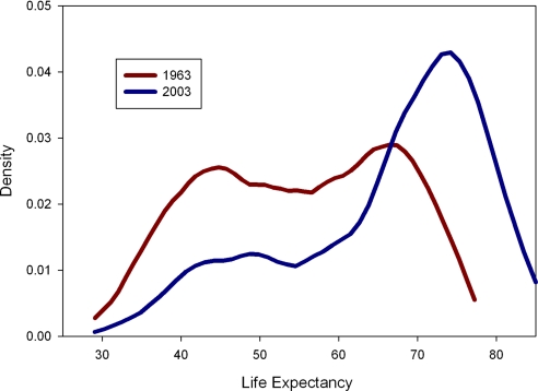
An examination of life expectancy in 1963 reveals twin peaks in the empirical distribution across countries: one group of countries clustered around a life expectancy of 40 years and a second group clustered around a life expectancy of 65 years. By 2003, the mode of each cluster had moved up by ≈10 years. Although the two groups are similar in that within each of them, there is progress toward higher life expectancy, a number of countries appear to have made the jump from the high-mortality cluster to the low-mortality cluster. We reject the hypothesis that these changes reflect a simple convergence process. The data instead suggest continuous advances among many countries within clusters, with advances in life expectancy in some nations resulting in a jump from one cluster to the other.

Recent studies suggest that since the late 19th century, gains in health have contributed more to human well being than has income growth (1, 2). Indeed, it is difficult to conceive of a more remarkable global human achievement over the past two centuries than the greater-than-doubling of life expectancy—from an initial level of ≈30 years in 1800 (3). This global trend appears to have accelerated in recent decades, with life expectancy increasing more than 10 years between 1963 and 2003, from 52.3 years to 66.0 years. Continued improvements are widely expected, with global life expectancy plausibly projected to reach 81 years by the year 2100 (4).

But these global trends mask considerable cross-country heterogeneity. Mayer-Foulkes (5) observes that life expectancy dynamics appear to generate a number of “convergence clubs.” These clubs consist of countries with similar life expectancy that also appear to experience relatively uniform sets of changes in life expectancy. McMichael et al. (6) focus on the most recent century and draw attention to three groups of countries: those that have experienced rapid improvement in their life expectancy, those that have experienced relative stagnation in their life expectancy, and those that have experienced an erosion of life expectancy. This trichotomy leads McMichael and his colleagues to argue against a deterministic process of global gains and convergence in population health. These findings notwithstanding, life expectancy has tended to rise fastest among countries that had low life expectancy in the 1960s. This suggests a narrowing of life expectancy gaps between countries and the prospect of long-run convergence in population health among countries (7–11).

We argue in this article that the life expectancy data reflect a dynamic that is more complex than a simple convergence process. The distribution of health in the world is bimodal, with a group of healthy, low-mortality countries and a group of unhealthy, high-mortality countries. We show that the process of catch-up and convergence in health between these two is not smooth; some high-mortality countries make a rapid transition to low mortality, whereas others appear to be stuck in a “mortality trap” where high mortality persists. We provide evidence of a critical value, or health threshold, which needs to be achieved for catch-up in health to occur. The existence of a critical value and its magnitude, which may be governed by both health and nonhealth dimensions of development, has important implications for how one should think about the sustainability of health and development and related policy interventions.

The central objective of this article is to construct a formal test of a single-regime versus a dual-regime trajectory of life expectancy. More specifically, we test a model of two convergence clubs, a high-mortality cluster and a low-mortality cluster, that allows for jumps between clubs (with a probability that may depend on initial life expectancy) against a model in which all countries follow the same continuous (although not necessarily linear) life expectancy trajectory. The data reject the latter model in favor of the two convergence club model. We find that all countries initially in the low-mortality cluster—that is, those with life expectancy of >55 years in 1963—have stayed in the low-mortality cluster. Some countries initially in the high-mortality cluster—with life expectancy of <55 years in 1963—have made, or are making, the transition to the low-mortality cluster, whereas others appear to be stuck in what we call a mortality trap.

Our results include a number of countries that have seen substantial declines in life expectancy since 1990 due to HIV/AIDS. However, our conclusions do not depend on the presence of HIV/AIDS; we show similar results using data on life expectancy that exclude the effect of AIDS mortality.

At the outset, we note also that our analysis identifies a mortality trap through a statistical analysis of levels and changes in country-level life expectancy data. It does not seek to offer or test hypotheses about the processes underlying the observed life expectancy patterns. We leave to future research the task of identifying possible factors (e.g., income growth, educational development, level and focus of foreign assistance, degree of democratization, governmental priorities, and budget allocations) that determine the critical value whose existence we seek to model and test.

Data

We rely on the Population Division of the United Nations for our data on life expectancy (12). The United Nations reports life expectancy figures for 192 countries at 5-year intervals over the period 1950–2005. The figures are based on the age-specific mortality rates prevailing within each 5-year interval. We follow the United Nations method and take life expectancy in 1963 (more precisely, at the beginning of 1963) to be that of the interval 1960–1965, whereas life expectancy in 2003 comes from the period 2000–2005. These are summary measures of the mortality schedule experienced by the population during the time interval and not the actual life expectancy of a true birth cohort.

The age-specific mortality rates are based on vital registration data, census age distributions, and survey information on infant mortality and deaths of other family members. When the availability of relevant data are limited, the United Nations may use model life tables to estimate life expectancy.

Although the United Nations life expectancy data are a widely used summary measure of population health, their quality may be poor, particularly in developing countries in the early period. This is due to under-registration of deaths, under-enumeration of the population and age misreporting in census data, and lack of survey data. Data are frequently missing and interpolated or extrapolated over time and even across countries (13). The introduction of the World Fertility Surveys in the 1970s, which were followed by the Demographic and Health Surveys, improved estimates of infant mortality. Data on adult mortality rates are at present often less reliable (14).

We use as our initial period the interval 1960–1965 and consider how life expectancy increased between this start date and the interval 1995–2000. We do not use data from the 1950s on the grounds that the data for this period appear to be of poor quality. All 192 countries for which data are available are used in our analysis.

Convergence

One way to think about convergence in life expectancy is to ask whether countries with lower initial life expectancy tend to experience larger subsequent gains in life expectancy than countries with higher initial life expectancy. If this were true, a regression of the change in life expectancy on the initial level of life expectancy would produce a negative coefficient β. This is known as β-convergence. Another approach is to consider the standard deviation, σ, of life expectancy across countries and ask whether this measure decreases over time. This is known as σ-convergence. The standard deviation of life expectancy across countries fell between 1960 and 1990 but has risen since 1990 because of the high HIV/AIDS mortality in countries that already had high mortality. We focus on β-convergence, which is necessary, but not sufficient, for σ-convergence.

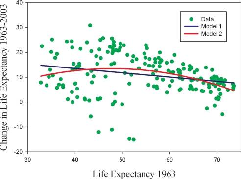
Fig. 1 shows the relationship between life expectancy in 1963 and subsequent gains in life expectancy between 1963 and 2003. The results, which are reported under Model 1 in Table 1, are a simple ordinary least squares (OLS) regression of the change in life expectancy on a constant and the initial level of life expectancy. Given initial life expectancy x_i in country i in the interval 1960–1965, the change in life expectancy over the period is defined as y_i. Our first model is linear.

where ε_i ∼ N(0, σ²). The negative coefficient on initial life expectancy implies β-convergence. The fitted line in Fig. 1 is the regression-predicted value and shows that we expect countries with low initial life expectancy to have a modestly higher increase in life expectancy on average.

Fig. 1.

Evolution of life expectancy, 1963–2003.

Table 1.

Models of change in life expectancy

	Model 1: Linear homoskedastic	Model 2: Quadratic heteroskedastic	Model 3: Two regimes, each linear homoskedastic
			High-mortality regime	Low-mortality regime
Constant	20.46 (7.79)	−20.55 (1.04)	57.19 (5.93)	48.80 (17.92)
Life expectancy 1963	−0.173 (3.71)	1.411 (2.03)	−1.218 (5.18)	−0.606 (13.3)
Life expectancy 1963 squared		−0.014 (2.45)
Standard error of the residuals	7.60		7.03	3.97
Residual error: Intercept		3.91 (12.5)
Residual error: Effect of initial life expectancy		−0.037 (6.45)
Probability of low-mortality regime: Intercept			−9.235 (3.91)
Probability of low-mortality regime: Initial life expectancy			0.203 (4.04)
Log likelihood	−660.7	−631.9	−601.6
N	192	192	192

Dependent variable: change in life expectancy 1963–2003. t statistics are in parentheses.

Although this specification is standard in the literature (5), it does not appear to fit the data very well. In particular, the largest gains in life expectancy did not occur in the countries that initially had the lowest life expectancy. Rather, countries in the middle of the initial distribution of life expectancy seem to have experienced the largest gains. In addition, there appears to be considerable variation in the life expectancy gains of countries that initially had low life expectancy, certainly in comparison with the relatively uniform health gains enjoyed in countries that had high initial life expectancy. This suggests that a better description of the process of improving life expectancy would allow for a nonlinear effect of initial life expectancy and for heteroskedastic residuals. We perform a quadratic regression allowing for an effect of initial life expectancy and its square. In addition, we allow for heteroskedasticity with the standard deviation of the residuals dependent on the initial level of life expectancy.

where ε_i ∼ N(0, σ_i²) and σ_i = e ^a+bx_i. The results are reported under Model 2 in Table 1. They show that both the coefficient on the squared term in the regression and the dependence of the standard deviation of the residuals on initial life expectancy are statistically significant. Fig. 1 also shows the fitted values from Model 2, which now predicts that the largest gains in life expectancy occur in countries in the middle of the distribution of initial life expectancy. We find that the relationship between the gain in life expectancy and initial life expectancy resembles an inverted “U,” with large gains in countries with life expectancy of ≈50 years in the interval 1960–1965 but lower gains for countries that initially had higher or lower life expectancy. The model also shows there to be great heterogeneity in the experience of countries with low life expectancy initially, with some achieving large increases in life expectancy while life expectancy stagnated or decreased sharply in others. Relative to Model 1, this nonlinear relationship provides a better description of the evolution of life expectancy. Instead of uniform convergence, there is convergence on average with, notably, the largest gains in life expectancy for countries that initially have medium life expectancy.

The Mortality Trap

Although the quadratic model fits the data better than a linear model, it is not clear that it provides a description of the data that could not be improved upon further (and meaningfully) by alternative models. We therefore consider some nonparametric methods for describing the life expectancy data. Fig. 2 shows the distribution of life expectancy across countries in 1963 and again in 2003 by using a kernel estimator. The striking feature of these plots is the existence of twin peaks in the distribution of life expectancy. For the interval 1960–1965, some countries cluster around a low level of life expectancy, whereas others cluster around a high level of life expectancy; somewhat fewer countries appear between these two groups. This bimodal distribution is still evident (although less so) in the interval 1995–2000. Wilson (11) finds twin peaks that weaken over time when the country data are weighted by population rather than weighted equally. Over time, the mode of life expectancy in each cluster increases. In addition, some countries appear to have “jumped” from the low- to the high-life-expectancy cluster, with corresponding changes in the size of their peaks.

Fig. 2.

Kernel density estimate of the distribution of life expectancy.

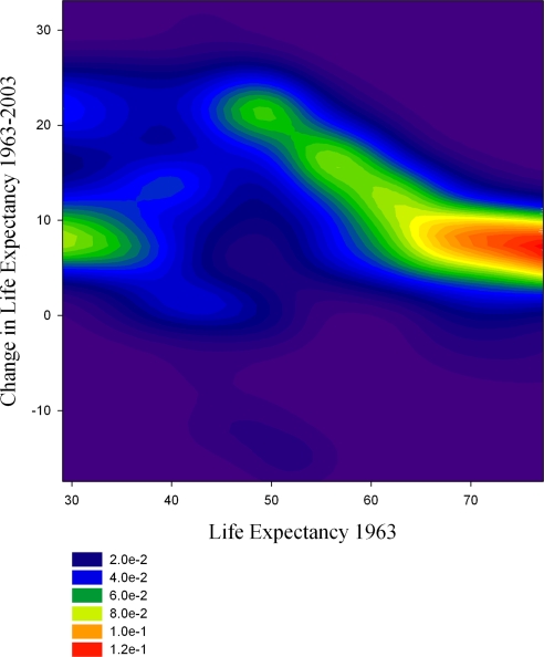
The explanation of Fig. 2 requires a more complex model of the evolution of life expectancy. We estimate the joint distribution of initial life expectancy and life expectancy change using a nonparametric kernel estimator. This allows us to construct an estimate of the empirical distribution of life expectancy changes conditional on a particular initial life expectancy. We do this for life expectancy at intervals of a half year.

Fig. 3 shows a contour map of the probability density of each increase in life expectancy, conditional on initial life expectancy. For initial life expectancies of <40 years, the modal gain in life expectancy is just under 10 years. For life expectancies of >50 years, there is a clear, downward-sloping relationship between initial life expectancy and the modal outcome, with a tight distribution of outcomes around the mode. For initial life expectancy of ≈50 years, the modal gain is just under 20 years, whereas for countries with initial life expectancy of 70 years, the modal gain is a more modest 7 years. Between initial life expectancies of 40 and 50 years, the distribution of the life expectancy gains appears to be very diffuse.

Fig. 3.

Conditional probability of life expectancy change by initial life expectancy.

Fig. 3 suggests a model with two regimes—one holding at high initial life expectancy and the other at a low initial life expectancy. We wish to examine this two-regime model formally and test it against the simpler single-regime models examined above. We assume that there are two regimes and that in each regime there is a relationship between initial life expectancy and the subsequent change in life expectancy. In theory, there could be a discontinuity as we vary initial life expectancy, with one regime holding below some critical value and another holding above it. Fig. 3, however, suggests that countries near the threshold have a chance of being in either regime. We allow for this by positing that there is a probability distribution that governs which state prevails for each country, where the parameters of the distribution are allowed to vary with initial life expectancy. These may reflect a genuinely random process; alternatively, one could imagine a process with a sharp discontinuity where the apparent randomness in outcomes is due to measurement error in initial life expectancy.

Formally, the model is

where ε_1i ∼ N(0, σ₁²) with probability 1 − λ_i.

where ε_2i ∼ N(0, σ₂²) with probability λ_i and

We allow for two distinct regimes. In each regime there a linear relationship between initial life expectancy and the improvement in life expectancy, but this relationship differs across regimes. The assignment of countries to regimes is random. The probability of being in a particular regime depends on initial life expectancy; we assume that the likelihood is a linear function of initial life expectancy, transformed into a probability by the cumulative normal distribution.

In most mixture models of this type, the probability of the different regimes is fixed and the same for each observation. In this model, we allow the probability of each regime to vary with the initial level of health. Our model is a simple special case of the dynamic regime switching model analyzed by Filardo (15). Provided that the true parameters are bounded, so that the regime variances are non-zero, and the probability of each regime is not uniformly zero, the model obeys the regularity conditions for an interior maximum of the likelihood function to be a consistent estimate of the model parameters, as shown by Kiefer (16) for fixed regime probabilities. Let θ = (α₁, α₂, β₁, β₂, σ₁, σ₂, ρ₀, ρ₁) be the parameters of the two-regime model. The likelihood function for the observation (x_i, y_i), given the model parameters θ, is

We use gradient methods to find the local maximum of the likelihood function starting from particular initial values of the parameters. The likelihood surface is not concave, and there are multiple local maxima. In addition, as the parameters approach the boundary of the feasible set (where one regime variance approaches zero, or the probability of one regime approaches zero for all values of initial life expectancy), the likelihood function becomes unbounded. Although the global maximum of the likelihood function lies on this boundary, we are interested only in the interior maximum that gives a consistent estimate. To address these issues, we initialize the gradient search procedure using a grid of initial parameter values. We discard outcomes where the gradient search algorithm converges to a boundary of the model, and we select the interior local maximum that gives the highest value of the likelihood function.

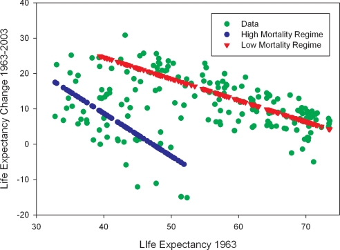
The results of our estimation are shown in the third column of Table 1. We estimate two regimes with very different intercepts. The linear relationship in each regime is graphed in Fig. 4 in the region where the probability of a country being in that regime exceeds 10%. The higher of the two regimes is downward sloping, giving much larger gains in life expectancy for countries with low initial life expectancy within that regime. The “mortality trap” regime (i.e., the lower one) is also downward sloping but gives smaller improvements in life expectancy at each level of life expectancy and has greater dispersion around the expected gain.

Fig. 4.

Change in life expectancy: Two regimes.

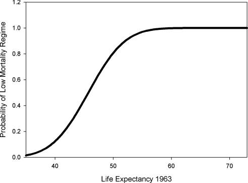
The probability of being in the mortality trap regime is shown in Fig. 5. Countries with life expectancy of >55 years in 1960 are almost certain to be in the “good” regime, whereas those with initial life expectancy of <35 years are almost certain to be in the mortality-trap regime. For countries with life expectancy between 35 and 55 years in 1960, there is a nontrivial probability of being in the good regime, as well as a nontrivial probability of being in the mortality trap regime. The sensitivity of the regime probability to initial life expectancy (dλ/dx) is highest at an initial life expectancy of 45.5 years.

Fig. 5.

Probability of low-mortality regime.

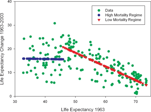
The declines in life expectancy in some countries evident in Fig. 4 are due to HIV/AIDS. It might be thought that the two-regime result simply reflects the differential impact of HIV/AIDS across countries. We therefore repeated our analysis using data from ref. 11 that give life expectancy with AIDS mortality removed. The results are presented in Table 2, and Fig. 6 shows the data and the two-regime model that we fit. The high-mortality regime now gives a fairly flat relationship with the gain in life expectancy appearing to be independent of the initial life expectancy. There is a sharp break in the relationship at a life expectancy of ≈46 years in 1963, with countries that are above this threshold having a downward-sloping relationship between initial life expectancy and the change in life expectancy. The transition between regimes is very rapid, and a strict threshold model also fits the data well (17).

Table 2.

Models of change in life expectancy: AIDS mortality removed

	Model 1: Linear homoskedastic	Model 2: Quadratic heteroskedastic	Model 3: Two regimes, each linear homoskedastic
			High-mortality regime	Low-mortality regime
Constant	30.71 (17.6)	−12.00 (1.28)	16.62 (1.76)	47.42 (19.3)
Life expectancy 1963	−0.319 (10.3)	1.336 (3.89)	−0.022 (0.09)	−0.582 (14.1)
Life expectancy 1963 squared		−0.015 (4.99)
Standard error of the residuals	5.03		5.55	3.89
Residual error: Intercept		2.40 (7.82)
Residual error: Effect of initial life expectancy		0.017 (3.03)
Probability of low-mortality regime: Intercept			184.2 (0.34)
Probability of low-mortality regime: Initial life expectancy			−4.06 (0.34)
Log likelihood	−581.8	−558.7	−552.9
N	192	192	192

Dependent variable: change in life expectancy, AIDS mortality removed 1963–2003. t statistics are in parentheses.

Fig. 6.

Change in life expectancy: Two regimes with AIDS mortality removed.

Although the two-regime models appear to fit the data quite well, we wish to test these against simpler single-regime models. The difficulties involved in testing the number of regimes are similar to those found when testing the number of components in a mixture of normal distribution (18). The distribution of the test statistic is nonstandard, because the parameters of the two-regime model are not identified under the null that a single-regime model describes the data; Monte Carlo methods and a parametric bootstrap are required to estimate the distribution of the test statistic (19). Given a null hypothesis of a single-regime model, we generate random data using the parameters estimated for the single-regime model. By generating repeated random samples of this type, and estimating the two-regime model using the methods described above on these generated data, we can generate the distribution of the test statistic under the null hypothesis.

Table 3 shows the critical values, based on 500 repetitions of the parametric bootstrap, of the likelihood ratio test statistic (twice the gain in log likelihood) as well as the actual test statistic. We reject both the linear and the quadratic single-regime models in favor of the two-regime model, even at the 1% significance level. When AIDS mortality is removed, we again reject both the linear and quadratic models in favor of the two-regime model, although in this case rejection of the quadratic model is at the 5% critical value.

Table 3.

Likelihood ratio test of a single regime versus two regimes

	Significance level	All mortality: Single-regime model		AIDS mortality removed: Single-regime model
		Linear model	Quadratic model	Linear model	Quadratic model
Critical values for testing the null of a single regime against alternative of a two-regime model	10%	24.8	3.8	24.9	7.6
	5%	27.2	5.5	26.7	9.6
	1%	34.6	11.0	31.5	13.3
Test statistic		118.2	60.6	57.8	11.6

Critical values from the empirical distribution under the null hypothesis using a Monte Carlo experiment with 500 replications.

Discussion

Our focus has been on the description of trends in national health. Countries with good health in the interval 1960–1965 appear to be making steady progress toward a high level of life expectancy. The countries within that group that had relatively poor health in the interval 1960–1965 had the largest health gains by the period 1995–2000. For countries exhibiting poor population health in 1960–1965, the story is more complex. Some countries have made modest progress over the last 45 years, whereas others have made large strides and now join the “good-health” group of countries. We model the process by which poor-health countries either succeed or stagnate in achieving gains in life expectancy as random but with a probability that rises with health status. This is suggestive of a threshold, whether at a certain level of initial health or in a combination of variables, at which countries are able to jump to the good-health regime. Below the threshold, countries are in a mortality trap. The trap is not absolute, because most countries in this regime also see gains in life expectancy and can hope to eventually move out of the high-mortality group.

Although we do not address the issue of what drives the observed patterns of health improvement, some existing research bears on the mechanisms behind takeoffs in health and their association with takeoffs in other measures of development. Pritchett and Summers (20) argue that rising incomes and education levels drive health improvements. By contrast, Preston (21) argues that population health gains are mainly due to an upward shift in the relationship between health and income, with improvements in health over time at each fixed level of income. This is likely due to more effective use of resources, either through technical progress or improved organization and allocation decisions. Jamison, Sandbu, and Wang (22) and Cutler, Deaton, and Lleras-Muney (23) emphasize the diffusion of health technologies and the implementation of public health measures that prevent the spread of infectious disease in developing countries. Health may also affect income levels (24), making it difficult to determine the direction of causality behind the observed association between health and income levels.

It is also important to note that changes in life expectancy may mask complex changes in the underlying schedules of age-specific mortality rates. In high-mortality settings, life expectancy is heavily influenced by mortality rates at young ages. On the other hand, Demetrius (25) and Keyfitz (26) show that reductions in mortality rates have less impact on life expectancy when life table entropy is low (i.e., when deaths are concentrated in a narrow age range). This situation typically occurs when life expectancy is high, making further gains in life expectancy more difficult. A more informative approach would be to focus on the movements in age-specific mortality rates. Unfortunately, long time series of age-specific mortality rates are only available for a small number of countries.

The “twin peaks” in the distribution of health seen in Fig. 3 mirror the twin peaks in the distribution of income (27). It may well be that takeoffs in health and takeoffs in income levels, as well as changes in other measures of social and economic development, happen contemporaneously. Yet, although socioeconomic indicators of national development are highly correlated in a cross-section of countries, Easterly (28) observes that, over reasonably long periods of time, development indicators can move quite differently within a country—considerable progress can occur in one dimension of development while other dimensions stagnate or even regress.

The existence of a threshold in health has important policy implications. Sachs's (29) argument for a sustained effort to aid African economies is based on the idea that these countries must escape a poverty trap. Similarly, the mortality trap justifies a “big push” approach to health to help countries reach and cross the low-mortality threshold. With limited resources, the largest health gains may be achieved by focusing on countries near the threshold, where small changes in health status can have large effects on those countries' chances of escaping the mortality trap. The threshold effect can also be used as an argument to support the International Finance Facility (30), which aims to increase current development aid by borrowing against future aid funding. This approach has considerable merit if the payoffs to spending that pushes countries quickly across a threshold are large in comparison to lower payoffs of incremental funding.

References

- 1.Becker GS, Philipson TJ, Soares RR. Am Econ Rev. 2005;95:277–291. doi: 10.1257/0002828053828563. [DOI] [PubMed] [Google Scholar]
- 2.Nordhaus W. In: Measuring the Gains from Medical Research: An Economic Approach. Murphy KH, Topel RH, editors. Chicago: Univ of Chicago Press; 2003. pp. 9–40. [Google Scholar]
- 3.Riley JC. Popul Dev Rev. 2005;31:741–764. [Google Scholar]
- 4.Lee RD. J Econ Perspect. 2003;17:167–190. [Google Scholar]
- 5.Mayer-Foulkes D. Convergence Clubs in Cross-Country Life Expectancy Dynamics. United Nations University, World Institute for Development Economics Research; 2001. Discussion Paper No 2001/134. [Google Scholar]
- 6.McMichael AJ, McKee M, Shkolnikov V, Valkonen T. Lancet. 2004;363:1155–1159. doi: 10.1016/S0140-6736(04)15902-3. [DOI] [PubMed] [Google Scholar]
- 7.Deaton A. In: Brookings Trade Forum 2004: Globalization, Poverty, and Inequality. Collins SM, Graham C, editors. Washington, DC: Brookings Institution Press; 2004. pp. 83–130. [Google Scholar]
- 8.Neumayer E. Struct Change Econ Dyn. 2003;14:275–296. [Google Scholar]
- 9.Sab R, Smith SC. IMF Staff Papers. 2002;49:200–211. [Google Scholar]
- 10.Hobijn B, Franses PH. Struct Change Econ Dyn. 2001;12:171–200. [Google Scholar]
- 11.Wilson C. Popul Dev Rev. 2001;27:155–171. doi: 10.1111/j.1728-4457.2001.00155.x. [DOI] [PubMed] [Google Scholar]
- 12.United Nations. World Population Prospects. United Nations, New York: Population Division; 2004. [Google Scholar]
- Bos E, Vu MT, Stephens PW, Patience W. Policy Research Working Paper Series. Washington, DC: World Bank; 1992. No. 851. [Google Scholar]
- 14.Hill K. Adult Mortality in the Developing World: What We Know and How We Know It. United Nations, New York: Population Division, Department of Economic and Social Affairs; 2003. [Google Scholar]
- 15.Filardo AJ. J Bus Econ Stat. 1994;12:299–308. [Google Scholar]
- 16.Kiefer NM. Econometrica. 1978;46:427–434. [Google Scholar]
- 17.Hansen BE. Econometrica. 2000;68:575–604. [Google Scholar]
- 18.Yungtai L, Mendell NR, Rubin DB. Biometrika. 2001;88:767–778. [Google Scholar]
- 19.McLachlan GJ. Appl Stat. 1987;36:318–324. [Google Scholar]
- 20.Pritchett L, Summers L. J Hum Resour. 1996;31:841–868. [Google Scholar]
- 21.Preston S. Popul Studies. 1975;29:231–248. [PubMed] [Google Scholar]
- 22.Jamison DT, Sandbu M, Wang J. Working Group 1 Discussion Paper No. 4. WHO, Geneva: Commission on Macroeconomics and Health; 2001. [Google Scholar]
- 23.Cutler D, Deaton A, Lleras-Muney A. J Econ Perspect. 2006;20:97–120. [Google Scholar]
- 24.Bloom DE, Canning D. Science. 2000;287:1207–1208. doi: 10.1126/science.287.5456.1207. [DOI] [PubMed] [Google Scholar]
- 25.Demetrius L. Proc Natl Acad Sci USA. 1974;71:4645–4647. doi: 10.1073/pnas.71.12.4645. [DOI] [PMC free article] [PubMed] [Google Scholar]
- 26.Keyfitz N. Applied Mathematical Demography. New York: Wiley; 1997. [Google Scholar]
- 27.Quah DT. Econ J. 1996;106:1045–1055. [Google Scholar]
- 28.Easterly W. J Econ Growth. 1999;4:239–276. [Google Scholar]
- 29.Sachs JD. The End of Poverty: Economic Possibilities for Our Time. New York: Penguin; 2005. [DOI] [PubMed] [Google Scholar]
- 30.HM Treasury. J Int Dev. 2004;16:865–878. [Google Scholar]