Estimation of synaptic conductances

Abstract

In order to identify and understand mechanistically the cortical circuitry of sensory information processing estimates are needed of synaptic input fields that drive neurons. From intracellular in vivo recordings one would like to estimate net synaptic conductance time courses for excitation and inhibition, g_E(t) and g_I(t), during time-varying stimulus presentations. However, the intrinsic conductance transients associated with neuronal spiking can confound such estimates, and thereby jeopardize functional interpretations. Here, using a conductance-based pyramidal neuron model we illustrate errors in estimates when the influence of spike generating conductances are not reduced or avoided. A typical estimation procedure involves approximating the current-voltage relation at each time point during repeated stimuli. The repeated presentations are done in a few sets, each with a different steady bias current. From the trial-averaged smoothed membrane potential one estimates total membrane conductance and then dissects out estimates for g_E(t) and g_I(t). Simulations show that estimates obtained during phases without spikes are good but those obtained from phases with spiking should be viewed with skeptism. For the simulations, we consider two different synaptic input scenarios, each corresponding to computational network models of orientation tuning in visual cortex. One input scenario mimics a push-pull arrangement for g_E(t) and g_I(t) and idealized as specified smooth time courses. The other is taken directly from a large-scale network simulation of stochastically spiking neurons in a slab of cortex with recurrent excitation and inhibition. For both, we show that spike-generating conductances cause serious errors in the estimates of g_E and g_I. In some phases for the push-pull examples even the polarity of g_I is mis-estimated, indicating significant increase when g_I is actually decreased. Our primary message is to be cautious about forming interpretations based on estimates developed during spiking phases.

1 Introduction

Primary goals of sensory neurophysiologists are to understand the dynamics of information processing and representation in various brain areas. What are the mechanisms (circuitry, synaptic and intrinsic cellular properties) that underlie sensory processing and that can account for the firing patterns of neurons? What are the relative contributions of feedforward and recurrent input, of the excitatory and inhibitory synaptic fields? What data are needed to develop and assess theories that can provide insights on mechanisms? We take a case-study approach here, the orientation tuning of visual cortex, and ask about the analysis of data that can give us reliable estimates of dynamic synaptic fields.

There are different theories about the wiring architecture of the primary visual cortex, mainly differing by the sensitivity to spatial phase in the coupling between cortical neurons. If we assume that the coupling is phase insensitive – see for instance the model studied in (McLaughlin et al., 2001; Wielaard et al., 2001) of a network of integrate-and-fire neurons in area 4Cα of V1– and we present a drifting grating stimulus, then, after phase averaging, both the inhibitory and the excitatory cortico-cortical conductances are almost constant over one cycle of the stimulus. On the other hand, a spatial phase selective coupling –see for instance the model built in (Troyer et al., 1998)– could produce an antagonistic temporal push-pull between excitatory and inhibitory cortico-cortical conductances.

To assess the sensitivity to spatial phase and possibly to distinguish two such mechanisms one relies on estimates of synaptic conductances, excitatory and inhibitory, that drive the neurons. Experiments that provide intracellular recordings, membrane potential time courses, of cortical cells are crucial in this regard. Several recent studies (Borg-Graham et al., 1998; Hirsch et al., 1998; Anderson et al., 2000; Anderson et al., 2001) are achieving this feat.

Recent theoretical studies (Rudolph and Destexhe, 2003; Rudolph et al., 2004) have shown how to estimate synaptic conductances in the presence of noise. In these approaches, as well as in (Borg-Graham et al., 1998), the estimates are obtained from subthreshold membrane potential recordings, thereby cautiously avoiding contamination by intrinsic conductances.

However, the presence of spikes is not always avoidable. In visual cortex, for example, experiments with drifting grating stimulation often evoke spiking activity in the cells, which cannot be easily prevented (say by hyperpolarizing a cell) or removed from the data. Sometimes, in experiments, one tries to remove this contamination of intrinsic conductances by filtering the membrane potential and, in some sense, clipping the spikes. For instance, in (Anderson et al., 2000) data analyzed with this procedure is interpreted as experimental evidence of the push-pull arrangement, thus supporting the phase selective coupling hypothesis. These conclusions are achieved by estimating the synaptic conductances through linear fittings of filtered membrane potentials, some of which show clear spiking activity. Mathematically speaking, the linear fittings are equivalent to the approximation that assumes averaged membrane potential depends linearly on the applied current. This approximation is only valid if the neuron is not spiking, as theoretical bifurcation diagrams can show (illustrated below in Fig. 5).

Figure 5.

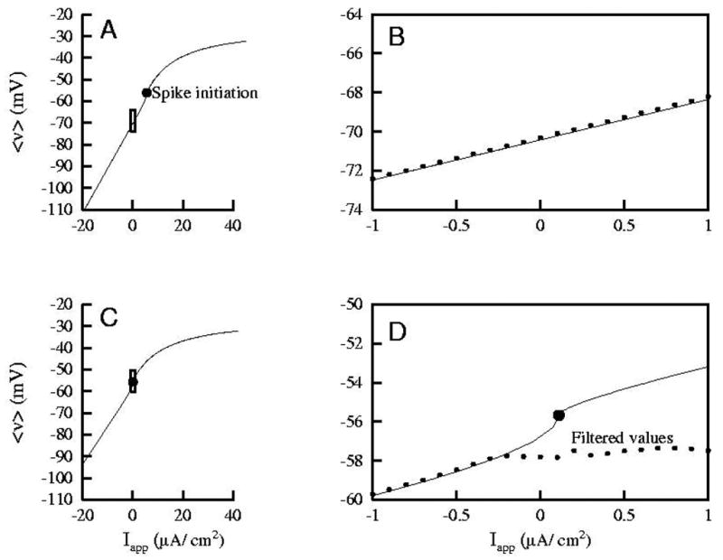
In A and C, we show theoretical I_app− < v > relationships for equation (1). They have been obtained after fixing, respectively, two representative pair of values (g_E, g_I )_i, i = 1, 2. Both pairs occur in specific moments of our simulations using the stochastic conductance input; bifurcation diagrams are computed using the AUTO feature of the package XPPAUT, see (Ermentrout, 2002). The filtering is the median of 21 values in a 5 ms window around the value. Observe that the I_app− < v > relationship is very close to linear when I_app is small enough (and so the neuron is not spiking). This linearity is clearly lost above the I_app value where repetitive spiking emerges (filled circle). This fact can be better appreciated in panels B and D, which are zooms of the small boxes in A and C, respectively. Panels B and D are restricted to a physiologically plausible interval I_app ∈ [−1, 1], the one where we have performed the computations of Figs. 6 and 7. Each value of the dotted curve in B (analogously, in D) is the filtered value of the membrane potential at the moment when (g_E, g_I ) = (g_E, g_I )₁ (resp., (g_E, g_I )₂). The fact that these values have been recorded during a simulation in which (g_E, g_I ) is not constant (values in panel B correspond to t = 20 ms in the right column of Fig.7 and values in panel D correspond to t = 51 ms in the middle column of Fig.7), means that the filtered values v_filt(t) do not capture the nonlinear conductance features of the spiking neuron: in D, the slope of the best linear fit of the dotted curve is far from the actual one (in fact the estimations of g_E and g_I have errors of 50% and 90%, respectively). The dotted curve would adapt to the theoretical curve if (g_E, g_I ) was constant. Instead, in B, we appreciate that the linear fitting works well since the cell does not spike for any of the I_app values.

In order to introduce some of the issues we outline the procedure. The main concern is how to accurately estimate the synaptic conductance g_syn and the synaptic reversal potential V_syn. A suitable procedure uses different steady current injections, denoted by I_app, to sample a portion of the cell’s current-voltage relation, < v > vs I_app (where < v > is the short-time-averaged voltage). When g_syn is dominant, the I_app− < v > curve would become linear and g_syn could be estimated using linear regression. By Ohm’s law, 1/g_syn would be the slope of the regression line. However, as seen in Fig. 1, the dominance of g_syn is not true when the cell is spiking. Accordingly, one could inject negative enough I_app current to prevent the cell from firing and then do the estimations of g_syn and V_syn. This is the case shown in the upper panels of Fig. 4. In contrast, the lower panels show the same estimation but using applied currents that do not prevent the cell from firing. It can be appreciated, then, that the estimation of the total conductance during phases of spiking is far from the value of g_syn.

Figure 1.

The membrane potential of a neuron model evolves rhythmically during 100 ms. Between the 10th and the 60th millisecond, an excitatory current of type I_syn = g_syn(v − V_syn), with g_syn = 0.05 mS/cm² and V_syn = 0 mV, is injected. Panel A shows the response of the cell during a 20 ms window (the inset shows a 100 ms period). For the same time interval, in panel B, we show the total ionic conductance, g_ion, the average of the ionic conductances, < g_ion>, the total synaptic conductance, g_syn, and the leakage conductance, g_l. Clearly the dominance of g_syn is broken significantly when the cell is spiking.

Figure 4.

We use a computational model of a cell with g_syn = 0.15 mS/cm² to test the procedures for estimating g_syn. The curves in the left panels (A, C) are the filtered membrane potentials of a neuron model; that is, after applying each current, we use a median-based filter, as in (Anderson et al., 2000), to obtain a smooth membrane potential that contains only small transients instead of the large spikes (we denote this smoothed potential by V_filt). The crosses on the right panels (B, D) show the three values of the filtered membrane potential, V_filt, obtained from the three injected currents shown in the respective left panels (A, C). The sloped line in the right panels (B, D) is a linear fit of the three values. In the upper panels (A, B), we apply injected currents that prevent the cell from firing and we obtain a good estimation of g_syn (the inverse of the slope is close to 1/0.15 ≈ 7). Contrary to the upper panels (A, B), in the lower panels (C, D) the injected currents do not prevent firing. Despite the filtering of the cell’s voltage, the estimations are far from satisfactory (for reference, the solid line on the righthand lower corner of D has the correct slope 1/0.15).

This is the simplest illustration of how and how not to estimate g_syn and V_syn. Apart from the problems reported above and illustrated by Fig. 4, there are other relevant factors:

• In general, both excitatory (g_E ) and inhibitory (g_I ) synaptic conductances are present. Thus four quantities are to be estimated: g_E, g_I, V_E and V_I. Since we can usually extract only information on two quantities (g_syn and V_syn), we must assume values for V_E and V_I to obtain g_E and g_I.

• The conductances g_E and g_I are time-varying, fluctuating around slowly varying means, as modulated by the drifting grating.

• The I_app range may overlap both the non-firing and the firing regime for different times, and so the I_app− < v > relationship will not be linear.

• Firing is stochastic and therefore the problem of how to properly average and smooth the membrane potential arises. See (Rudolph and Destexhe, 2003; Rudolph et al., 2004) for an estimation of the conductances from a noisy hyperpolarized membrane potential using Ornstein-Uhlenbeck processes and Fokker-Planck equations.

Here, we evaluate the accuracy of conductance estimates. We consider a conductance-based model of a pyramidal cell together with two different input scenarios of excitatory/inhibitory conductances (see Methods): a smooth and idealized push-pull arrangement of excitation and inhibition (smooth conductance input) and a stochastic arrangement obtained from a computational network (stochastic conductance input).

In the Results section, we analyze the usual procedure of linear estimation of conductances and give a mathematical explanation of the errors in the estimations obtained in this way. These problems appear clearly when applying the procedure to the spiking cell model subjected either to the smooth conductance input or to the stochastic conductance input. In both cases, when the cell model is spiking the disagreement between the estimated conductances and the actual prescribed ones is apparent.

2 Methods

Our computational experiments are carried out with a model for a single cortical neuron and two prescribed synaptic drives: the first (which we call smooth conductance input), made up by mimicking smooth time courses of the synaptic excitatory and inhibitory conductances (related to one possible wiring architecture in primary visual cortex); the other synaptic drive (which we call the stochastic conductance input), is obtained from the activity of a computational network of about 16 000 neurons, see (Tao et al., 2004). Our cell model serves as ”reporter cell”, that behaves as a specific cell of the network responding to the network-generated synaptic field, reminding us of an in silico version of the dynamic clamp technique. The network itself takes into account stochastic effects and so, the synaptic input that our cell receives is noisy.

For the purpose of this paper, the main features can be observed in both prescribed synaptic input scenarios, somewhat more transparently in the case of the smooth conductance input. However, the time course variability of conductances in the stochastic conductance input shows features which are associated with less idealized situations.

2.1 Adapted pyramidal cell model

We will use a Hodgkin-Huxley type model (HH model) which describes the activity of a cortical pyramidal cell. We adapt a simplification of Traub’s model, borrowing the values for the characteristic conductances from (Wang, 1998). Compared to Wang’s two-compartment model in (Wang, 1998) our version includes the soma compartment only; we have removed the dynamic equation for the calcium concentration and brought the gating variable m to its steady-state, m = m_∞(v). The resulting model contains both a sodium and a potassium current, which drive the membrane potential during spiking.

The current-balance equation for the membrane potential, v = v(t), is:

$$C_m\frac{dv}{dt}=-I_L-I_{Na}-I_K-I_{\mathit{syn}}+I_{\mathit{app}}.$$ (1)

Equation (1) contains the synaptic current (I_syn) and a constant applied current (I_app), controlled by three parameters: the two (excitatory and inhibitory) synaptic conductances and the intensity of I_app. The ionic currents in (1) are given by:

$$\{\begin{array}{l}{I}_L\hspace{0.17em}\hspace{0.17em}\hspace{0.17em}=g_L(v-V_L),\hfill \\ I_{Na}\hspace{0.17em}\hspace{0.17em}\hspace{0.17em}=g_{Na}\hspace{0.17em}{m}_{\infty }^3(v)\hspace{0.17em}h\hspace{0.17em}(v-V_{Na}),\hfill \\ I_K\hspace{0.17em}\hspace{0.17em}\hspace{0.17em}=g_K\hspace{0.17em}{n}^4\hspace{0.17em}(v-V_K).\hfill \end{array}$$

The gating variables h and n satisfy the usual type of differential equation:

$$\frac{dw}{dt}=\phi [{\alpha }_w(v)\hspace{0.17em}(1-w)-{\beta }_w(v)\hspace{0.17em}w]=\phi \frac{w_{\infty }(v)-w}{{\tau }_w(v)},$$ (2)

where w represents either h or n. In general, $w_{\infty }(v)=\frac{{\alpha }_w(v)}{{\alpha }_w(v)+{\beta }_w(v)}$ and ${\tau }_w(v)=\frac{1}{{\alpha }_w(v)+{\beta }_w(v)}$, where:

$$\begin{array}{ll}{\alpha }_h(v)\hspace{0.17em}\hspace{0.17em}\hspace{0.17em}=0.07\hspace{0.17em}exp\hspace{0.17em}(-(v+50)/10),\hfill & {\beta }_h(v)\hspace{0.17em}\hspace{0.17em}\hspace{0.17em}=\frac{1}{1+exp\hspace{0.17em}(-0.1\hspace{0.17em}(v+20))},\hfill \\ {\alpha }_n(v)\hspace{0.17em}\hspace{0.17em}\hspace{0.17em}=-0.01\frac{v+34}{exp\hspace{0.17em}(-0.1\hspace{0.17em}(v+34))-1},\hfill & {\beta }_n(v)\hspace{0.17em}\hspace{0.17em}\hspace{0.17em}=0.125\hspace{0.17em}exp\hspace{0.17em}(-(v+44)/25),\hfill \\ {\alpha }_m(v)\hspace{0.17em}\hspace{0.17em}\hspace{0.17em}=-0.1\frac{v+33}{exp\hspace{0.17em}(-0.1\hspace{0.17em}(v+33))-1},\hfill & {\beta }_m(v)\hspace{0.17em}\hspace{0.17em}\hspace{0.17em}=4\hspace{0.17em}exp\hspace{0.17em}(-(v+58)/12).\hfill \end{array}$$

The biophysical parameters that we fix throughout and the units are the following:

Conductances	gL = 0.1, gN a = 45, gK = 18	mS/cm2
Reversal potentials	VL = −65, VN a = 55, VK = −80, VE≈ 0, VI≈ −80	mV
Capacitance	Cm = 1	μF/cm2
Non-dimensional constant	φ = 4
Applied currents		μA/cm2

2.2 Synaptic drive

The computational model that we have described above will be driven by synaptic inputs of type I_syn = g_E (v − V_E ) + g_I (v − V_I ), where g_E = g_E (t) and g_I = g_I (t) represent, respectively, the sum of all excitatory and inhibitory conductances received by our neuron model.

We present results using the two different types of prescribed time courses (g_E (t), g_I (t)): the smooth conductance input and the stochastic conductance input. We describe them next.

2.2.1 The smooth conductance input, a model of phase selective coupling

The smooth conductance input tries to mimic the excitatory and inhibitory conductances obtained after assuming a phase selective coupling in the visual cortex, which leads to a push-pull temporal relation between excitatory and inhibitory cortico-cortical conductances. On the other hand, the LGN impinges on the cortical cells over half of the cycle (in an excitatory way). We have represented this fact by specifying the LGN input conductance to trace a downward (negative curvature) parabola in the first half of the cycle. The pushes and pulls of the synaptic conductances have been mimicked using parabolas with different amplitudes. To simulate the effect of different orientations of the drifting grating stimuli, we have introduced a parameter to modulate excitation through both the LGN input and the cortico-cortical excitation by increasing the amplitude of the above mentioned downward parabola. The inhibition has the same temporal profile for all values of this parameter. Typical (g_E (t), g_I (t)) temporal profiles and the respective responses of the cell (1) are given in Fig. 2. The same inputs are used in Fig 6. One can imagine that the smooth time courses of g_E (t) and g_I (t) are due to an average across the afferent population.

Figure 2.

Responses of model (1) for three different levels of excitation (decreasing from the top to the bottom) in the smooth conductance input. These levels of excitation try to simulate the effect of different drifting grating’s orientations.

Figure 6.

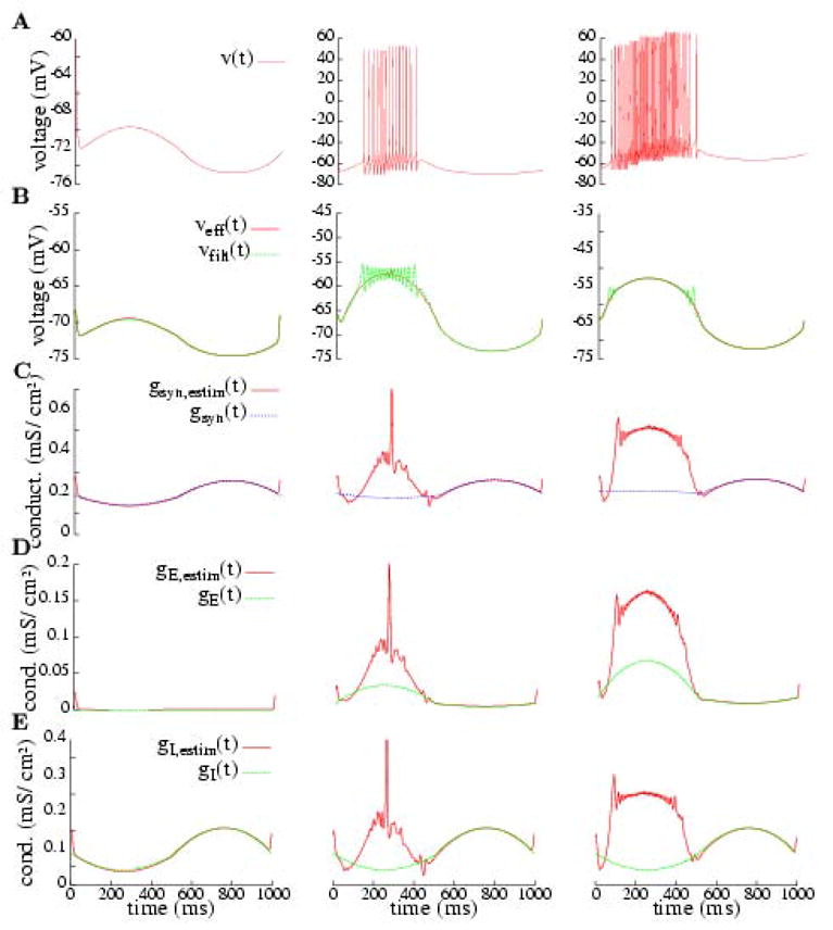
Estimation of effective reversal potential and conductances for background and for two different levels of stimulation: for the smooth conductance input under model (1). The simulation is carried out over a 1 second cycle. The filtering is a Gaussian one (see Appendix A and Fig. 8) that performs a better smoothing in the case of regular firing patterns. The first column shows the cell model’s background behavior. The second and third columns correspond to different levels of excitation (see Fig. 2 to see the specified conductance profiles, which coincide with the green curves in rows D and E here). (Row A) Response of the cell under the different situations. (Row B) Estimated reversal potential compared to the response in A filtered; the estimation is fairly good, as we predict. (Rows C, D and E) Estimated conductances (total synaptic, excitatory and inhibitory) compared to the actual (specified) ones; the estimations fail when the cell is spiking. Legend: v(t): membrane potential; V_eff (t): estimated membrane potential; v_filt(t): filtered actual membrane potential; g_syn,estim(t): estimated total synaptic conductance; g_syn(t) = g_E (t) + g_I (t) + g_l: actual total synaptic conductance; g_E,estim(t): estimated excitatory synaptic conductance; g_E (t): actual excitatory synaptic conductance; g_I,estim(t): estimated inhibitory synaptic conductance; g_I (t): actual inhibitory synaptic conductance.

2.2.2 Conductances from a spiking network (stochastic conductance input)

In order to have a more realistic situation, inducing sparse spikes rather than repetitive firing (thus contrasting with the smooth conductance input) and, also, to observe the influence of stochasticity, we use the conductances profiles from a computational network model of V1 with 128² integrate-and-fire neurons (Tao et al., 2004; McLaughlin et al., 2001; Wielaard et al., 2001). In particular, we have chosen one cell, representative of the cells of the layer 4Cα of the primary visual cortex. We call it the reference cell.

Once the reference cell of the network is selected, its conductance time courses are inherited by the reporter cell that we are simulating, that is: we drive the cell modeled by equation (1) with the “actual” (g_E (t), g_I (t)) of the reference cell. In other words, if we consider the HH model and the conductances received, say, by a complex excitatory cell of the network, we are studying how a “typical” complex HH-like excitatory cell would behave in the network-generated synaptic field. This reporter cell does not send impulses to the others; it is thought of as purely postsynaptic in the network.

For the reference cell in (Tao et al., 2004), we collect the conductance time courses after presenting different drifting gratings at 8 Hz. After a simulation of the network, we extract the time courses of both the excitatory and the inhibitory conductances that the cell receives under each stimulation and use them to drive our HH model reporter cell.

In Fig. 3 we show some temporal profiles of synaptic conductances that we inject to our computational neuron, along with the resulting membrane potentials. For the sake of brevity, only the preferred and the orthogonal to preferred drifting gratings are presented. The time interval is [0, 125] ms because the procedure we apply to the data implies an average over 8 cycles (since the stimulus comes from a 8 Hz drifting grating).

Figure 3.

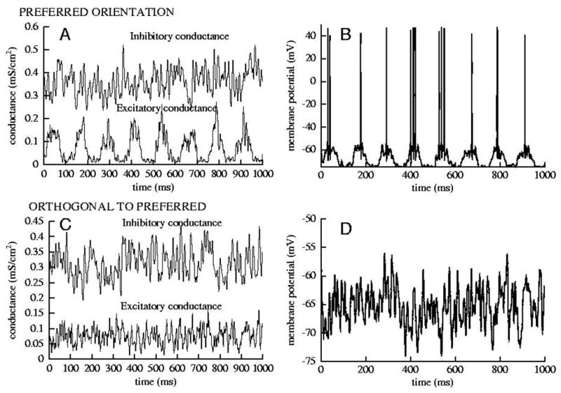
(A) The conductances received by a selected cell of the stochastic conductance input under a drifting grating at the preferred orientation of this selected cell. (B) Response of the HH model cell to the stimulus plotted in A. (C) Input conductances from a drifting grating, orthogonal to the preferred orientation. (D) Response of the HH model cell to the stimulus plotted in C. These input conductances are the same used in Fig. 7.

2.3 Numerical methods

All the computations are carried out using a 4th order Runge-Kutta method with a fixed step size Δt = 0.05 (ms). In Appendix A we also describe the smoothing techniques that have been used.

3 Results

This section is divided into three parts. We first illustrate the response of the pyramidal cell model given by (1) for different synaptic drives, constant as well as the two time-varying drives described in Section 2.2; secondly, we describe and analyze the typical methodology for obtaining the estimates of the conductances; and, finally, we examine these computed estimates under the two different dynamic synaptic drives. The strategy consists of considering known conductance profiles to stimulate a neuron and, afterwards, re-estimate these conductances to evaluate the errors.

3.1 Conductances time courses: synaptic and intrinsic. Confounding factors in estimation

When estimating synaptic conductances, one needs them to be dominant. However, as the time courses of conductances in Fig. 1 show, when the cell is spiking, the ionic conductances can be transiently very large. A direct estimation of the synaptic conductances from intracellular measurements, thus, seems inaccessible.

Realistic input conductances received by a cell are not as simple as those of Fig. 1. Next, in Figs. 2 and 3, we show the responses to two types of synaptic drive scenarios (smooth conductance input, stochastic conductance input) that we will use to test the linear estimation technique. In Fig. 2, for the smooth conductance input, we see increased firing during the phase of excitation as the amplitude of g_E (t) increased (top row to bottom row) the amplitude. In this case the slowly and smoothly varying conductances lead to continuous variations in instantaneous firing rate. Note the anti-phase behavior of g_I (t). For the case of stochastic conductance input, in Fig. 3, the response is shown under stimulation by two different drifting gratings (preferred and orthogonal to preferred). In this case only a few spikes per cycle, even for the preferred orientation, are generated; the membrane potential fluctuations resemble those as seen in experiments.

3.2 Applying the methodology for estimation of synaptic conductances to a neuron model

As explained in the Introduction, in recent works experimental researchers have coped with the problem of estimating the synaptic conductances in primary visual cortex, see (Borg-Graham et al., 1998) and (Anderson et al., 2000), for instance, as relevant information to unveil the wiring architecture of V1. At times, spiking is unavoidable and can lead to important misinterpretations of the data. We illustrate this point in computational models and suggest how to reduce the problems.

3.2.1 Linear procedure to estimate the synaptic conductances and the effective reversal potential

The standard estimation procedure (filtering plus linear regression) can be described through the following steps: (1) Stimulation of cells through drifting gratings (in experiments) or input conductances (in numerical simulations). As a consequence, the cell’s membrane potential, v(t), is recorded (in experiments, intracellularly). The time of recording is chosen to be a multiple (M) of the drifting period; (2) Use of a low-pass filter to clip the spikes and smooth the membrane potential; (3) Average the membrane potential over the M cycles; we call v_filt(t) the final outcome. Observe that v_filt is defined over 1 cycle; (4) Estimation of the total synaptic conductance and the effective reversal potential; (5) Estimation of the excitatory and the inhibitory synaptic conductances.

Step 1 is exclusively experimental and step 3 does not require further explanation. A discussion about filtering (i.e, step 2) is given in Appendix A. Thus, we will focus here on the details involved in the two remaining steps, 4 and 5.

The procedure to estimate the total conductance consists of applying several (N) injected currents $I_{\mathit{app}}^{(j)}$, where j = 1, …, N, and smoothing the resulting membrane potentials, v^(j)(t). After that, if the stimulus is periodic in time, an average over the M cycles is required to obtain what we will call $v_{\mathit{filt}}^{(j)}(t)$. Hence, for each t, we have a set of pairs ( $I_{\mathit{app}}^{(j)},v_{\mathit{filt}}^{(j)}(t)$).

In this paper, we will always consider $I_{\mathit{app}}^{(j)}=-1+(j-1)/10\hspace{0.17em}\mu A/c{m}^2$, for j = 1, …, 21, that is, I_app ∈ {−1, −0.9, −0.8, …, 0.9, 1} μA/cm². We choose this interval to be realistic; this choice is justified in Appendix B. For each current, we have filtered the membrane potential over 1 second. For the stochastic conductance input, the stimulus comes from a drifting grating at 8 Hz and so, we will average over the 8 cycles (step 3). For a preview of the result after this last average, see Fig. 7. For the smooth conductance input, since it does not contain stochasticity, a single cycle stimulus is presented and so we do not need to average after smoothing.

Figure 7.

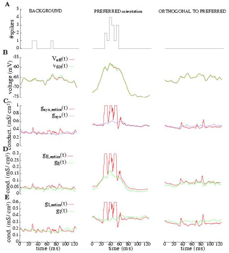
Estimation of effective reversal potential and conductances for background and two different drifting gratings applied to the stochastic conductance input on model (1). We average over the 8 cycles of 125 ms, given by the temporal frequency (8 Hz) of the drifting grating. The filtering is the median of 21 values in a 5 ms window around the value; this filtering is more effcient than the Gaussian one when the spikes are sparse. The first column shows the cell model’s background behavior. The second and third columns correspond to preferred and orthogonal to preferred drifting gratings, respectively (see Fig. 3 to see the conductance profiles injected). (Row A) Histogram of the model’s spike response (in bins of 5 ms.) under the different situations. (Row B) Estimated reversal potential compared to the response in A filtered; the estimation is fairly good, as we predict. (Rows C, D and E) Estimated conductances (total synaptic, excitatory and inhibitory) compared to the actual ones (injected); the estimations fail when the cell is spiking. The estimated conductances are clipped in amplitude in order to allow visual comparison on these plots; their peak values (in mS/cm²) are: max g_syn,estim≈ 8.83, max g_E,estim≈2.79, max g_{I,estim ≈} 5.94. See caption of Fig. 6 for the legends.

The estimation procedure is motivated as follows. If the solutions of the system of differential equations ((1)-(2)_h,n) are close to the steady state (a critical point representing a hyperpolarized state), then the activity of the ionic channels is negligible and also, &vdot; ≈ 0. Hence, from (1) we would have

$$0\approx -g_L(v-V_L)-g_E(v-V_E)-g_I(v-V_I)+I_{\mathit{app}},$$

and so

$$v(t)\approx V_{\mathit{eff}}(t)+\frac{I_{\mathit{app}}}{g_{\mathit{syn}}(t)},$$ (3)

where

$$V_{\mathit{eff}}(t)=\frac{g_E(t)V_E+g_I(t)V_I+g_L{V}_L}{g_{\mathit{syn}}(t)}\hspace{0.17em}\hspace{0.17em}\hspace{0.17em}\text{and\hspace{0.17em}}\hspace{0.17em}\hspace{0.17em}{g}_{\mathit{syn}}(t)=g_E(t)+g_I(t)+g_L.$$ (4)

Then, thinking of (3) as $v(t)=v(t;I_{\mathit{app}})\approx V_{\mathit{eff}}(t)+\frac{1}{g_{\mathit{syn}}(t)}{I}_{\mathit{app}}$, we realize that g_syn(t) corresponds approximately to the inverse of the slope of v(t; I_app) and V_eff (t) to the intercept v(t; 0), see Fig. 4 (panels B and D) for an illustration. Hence, we can have an indirect measure of the total synaptic conductance, g_syn,estim(t) := g_syn(t), and the effective reversal potential, V_eff (t), by linearly fitting at each point in time the relation between the injected current and the membrane potential.

Once g_syn(t) is estimated, still neglecting possible spiking conductances, the excitatory (g_E (t)) and inhibitory (g_I (t)) synaptic conductances can be estimated from equations in (4) – assuming that values for V_E, V_I and g_L are known.

Figure 4 shows a simple application of the procedure to obtain g_syn(t) for a fixed t. The upper panels (A, B) show a case of accurate estimations (the cell model is not spiking at all), while the lower ones (C, D) illustrate inaccurate estimations due to the presence of spikes for some of the I_app values.

So far, the basis of the method and its first handicaps (see Fig. 4-D) have been presented; now, we are going to analyze its validity in more detail.

3.2.2 Analysis of the procedure

The method obviously works well when the synaptic activity is exclusively driving the system because, then, (3) holds. However, when the cell is spiking or close to spike initiation or when only the potassium channels are open (thus hyperpolarizing), the presence of intrinsic conductances invalidates (3) and the linear relation between v and I_app is broken. As an attempt to avoid this problem, intracellular spiking voltage recordings are often filtered (obtaining v_filt(t) according to step 2 above mentioned) in order to clip the spikes and get rid of intrinsic conductances. However, our claim is that, even with this filtering, there is in general not a linear relation between v_filt(t) and I_app.

Because of the stochasticity of the signal, both in the experiments and in some of our simulations, a median-based filtering is used (see Appendix A for more information).¹

For theoretical analysis of potential diffculties, we consider the mean voltage (< v >) as a third filter (only used in Fig. 5). For fixed conductance inputs (g_E (t) = g_E,0, g_I (t) = g_I,0), we have performed a comparison between the data filtered with a median-based filter and those filtered with a mean-based one. Both provide very similar I_app− v_filt curves. Thus, the I_app− < v > curves constitute a solid basis for our theoretical arguments. ²

Figure 5 displays a typical I_app− < v > relationship for the model cell ((1)-(2)_h,n). It shows that even with a good estimation of the average membrane potential (< v >) through filtering, the conductance would not be well estimated: observe that the slope of the solid line in panel D is not the same before and after the spike initiation point.

According to the I_app− < v > relationship shown in Fig. 5, we observe that if the cell is not spiking for any injected current, then the ( $I_{\mathit{app}}^{(j)}$, v^(j)) values fit to a straight line, whose slope accurately estimates the inverse of the total synaptic conductance, see panel B in Fig. 5. On the other hand, if the cell is spiking for some injected current, then the ( $I_{\mathit{app}}^{(j)}$, v^(j)) values lie on a non-linear curve (the solid curve in panel D).

Apart from the nonlinear nature of the I_app− < v > curve, panel D in Fig. 5 also displays another contaminating factor. The dotted points in panel D come from the values of the actual g_E and g_I curves at t = 51 ms in Fig. 7, middle column. For I_app ≤ I *, where I * ≈ −0.3 μA/cm², the stimulus does not elicit spikes for these values of g_E and g_I ; it can be observed that the dots where I_app ≤ I * are perfectly located on the theoretical curve. However, when I_app is big enough and spikes are elicited close to t = 51 ms, then the filtered values (dots) disagree with the theoretical predictions. This fact indicates that, for stochastic conductance inputs, there is an extra source for the contamination of conductances.

Summarizing, we claim that the method is only valid for those values situated in the non-spiking zone for all the injected currents because the approximation in formula (3) is not valid in the other regimes. In particular, the conclusions drawn from linear estimations of filtered spiking intracellular recordings are not valid. The problems reported here persist under different types of filterings, under background conditions (not shown here) and kinds of synaptic inputs, as will be further seen in the simulations of Section 3.3. Before describing these results, we present more detailed information about the sources of inaccurate estimates.

3.2.3 Sources of overestimation and underestimation

In Fig. 5-D, a case in which for some I_app values between −1 and 1 the cell is spiking, we have noticed that the fitted line would have quite a different slope from 1/g_syn. In particular, the values of the voltage for I_app> I * lie below the theoretical curve. Then, the slope is lower and one will overestimate the total conductance. This is the most typical case of inaccurate estimation in “realistic” neurons (because it is related to the presence of isolated spikes), and explains why later (Fig. 7) we will encounter such overestimations.

The other case of overestimation arises in smoother input profiles like the smooth conductance input. Here, one frequently observes that although linear fittings are decent the inverse of the fitted slope is far from the total synaptic conductance. This occurs, for example, when all the injected currents induce spikes which are contained in a small enough interval of I_app-values (see for instance the center of the spiking regions of the estimations in Fig. 6; middle panel of rows C, D and E). In this case all the ( $I_{\mathit{app}}^{(j)}$, v(j)) points lie close to some small region on the curved part of the < v > − I_app curve, away from the onset of repetitive spiking. There, the slope is smaller than that of the non-spiking region (see panel D in Fig. 5 for the theoretical prediction) and so, leads to an overestimate of the inverse of its slope.

Of course, in the region on the steepest part of the I_app− < v > curve, the total conductance would be underestimated, but this is not so frequent and, when it happens, the filtering process has also a strong influence. The clearest examples are in Fig. 6, just on the limits of the spiking domains. Here we are filtering a single membrane potential for the smooth conductance input and, when we are close to the region of spiking onset, we use points that sample action-potentials to filter non-spiking points and vice versa. This fact can give, for non-spiking points close to the spike initiation, some mean values larger than the predicted ones, thus inflating the slope of the fitted line and so underestimating the inverse of the slope.

3.3 Estimating synaptic conductances for simulated orientation-tuned responses of cortical (V1) neuron model to drifting grating

In this section, we show several simulations using equation (1) with the two types of conductance inputs described in Subsection 2.2. Up to this point, we have analyzed the local problems that can arise. Here, we want to focus on the “macroscopic” effects through examples.

The relative roles of inhibition and excitation are key to understanding the wiring architecture of the cortex. In recent years, some experimental data on intracellular v(t) have been used to estimate the time courses of (g_E (t), g_I (t)). We will simulate the response of the neuron model to the two idealized inputs. As suggested in Section 3.2.2, our results will show that the methodology can lead to considerable mis-estimates, and thereby a loss of support for some interpretations. The two types of inputs (smooth conductance input and stochastic conductance input) should be thought of as net input to a cortex cell that includes both thalamic and intracortical interactions. In both cases, the thalamus sends excitation to our cortical cell model in half of the period. In the case of the smooth conductance input, the period is 1000 ms, while for the stochastic conductance input it is 125 ms (in fact, the simulation runs for 1000 ms, but we average over 8 cycles to reduce stochasticity).

In Figs. 6 and 7 we present the results in a compact way, where the panels are organized as follows. Each column corresponds to a different presentation of stimulus (each stimulus producing a different level of excitation on the cell). The first row (A), in Fig. 6 is the response elicited by the cell and, in Fig. 7, it is a histogram of the number of spikes; the second row (B), shows the measure of the smoothed and averaged membrane potential for I_app = 0 compared to the estimated effective reversal potential from (3); the third row (C), contains a panel with the prescribed total synaptic conductance, g_syn = g_E + g_I + g_l and the total conductance estimated from (3), g_syn,estim; finally, in the fourth and fifth rows (D, E) we compare (respectively) the prescribed excitatory and inhibitory conductances with the ones estimated from (4).

3.3.1 Smooth conductance input: specified smooth time courses, with g_E and g_I in push-pull antagonism

The smooth conductance input has been modelled to mimic the antagonism between excitatory and inhibitory cortico-cortical inputs. It is not intended to be realistic, but a paradigm for this antagonism. The conductance inputs in this case separate clearly a spiking domain and a non-spiking one. This allows to better distinguish the different quality of the estimations, as we have discussed in Subsection 3.2.

In Fig. 6, we can clearly appreciate that when the synaptic currents dominate the activity of the cell (e.g., t ≳ 500 ms for the last column) the estimations are correct. On the other hand, the estimations fail when in spiking regimes (although sometimes the linear fittings are well correlated). The estimates of g_E (t) (row D) can be in error by factors of 2–4. The mis-estimates of g_I (t) during spiking are more severe, failing to even correctly indicate the polarity in g_I swings. According to the estimated time course, g_I is peaking and comparable to g_E during the spiking phase when actually g_I is dipping then. Finally, in the transition between spiking and non-spiking (e.g., close to t = 500 ms in row E third column), a kind of underestimate (undershooting) is observed; here, the correlation of the linear fitting is very poor.

3.3.2 Stochastic conductance input: stochastic inputs from network simulation

In Fig. 7 we present the estimations of conductances and effective reversal potential for the stochastic conductance input to our cell. We have used the median filter with a 5 ms window and then averaged over the eight cycles (125 ms each cycle).

The inaccuracies indicated in Subsection 3.2 are evident: the estimations of conductances are pretty good when the membrane potential remains under threshold, but fail in the neighborhood of a spike. This fact can be better appreciated in the second column of Fig. 7, corresponding to a drifting grating at preferred orientation that induces a strong response. The correlation between the spiking regions and the inaccurate estimates is very clear in the second column between 20 and 60 ms, where the estimated g_E and g_I can be 15–20 times larger than the actual values (note, the estimated time courses have been clipped for plotting purposes).

4 Discussion

In this paper we have revisited the methods for the estimation of conductances and have obtained a clear conclusion: the estimation of conductances is only reliable if based upon intracellular measurements when intrinsic (spike-generating) currents are negligibly small. Frequently in the literature, the validity of these methods of estimation is based upon a comparison of the estimated effective reversal potential and the actual filtered potential; that is, the agreement of these two potentials is taken to indicate that the estimates of the conductances will be accurate. However, our analysis further shows that, in fact, this does not follow. As shown in row B of Figs. 6 and 7, one frequently has agreement between the estimated reversal potential and the actual filtered potential, and yet no accuracy in the estimates of the conductances.

To understand this, notice that in (3) we are estimating V_eff directly, while g_syn is estimated through its inverse. Then, if we have an absolute error ε in the estimation of V_eff, the relative error (the proper measure because our plots have the scale determined by their magnitudes) will be ε/V_eff approximately. Since |V_eff| is typically around 60--70 mV, the relative error is reduced with respect to the absolute error between 1 and 2 orders of magnitude. On the other hand, if we have the same error in estimating 1/g_T, then the absolute error in estimating g_T is of the order of ε $g_T^2$. When the conductances are high (as they are in visual cortex under high contrast stimulation), the error is amplified. Quantitative measures of these errors in the numerical simulations have confirmed a good performance for the estimation of V_eff (less than 5% error) and dramatic errors (more than 100% in the presence of intrinsic conductances) for the estimation of the g_syn, g_E and g_I (see again Fig. 6 and 7 and Subsection 3.3).

Accurate estimates of the excitatory and inhibitory conductances can provide significant information about the wiring architecture of the cortex. For example, in (Anderson et al., 2000) these methods are used to estimate the excitatory and inhibitory conductances, and the results are interpreted as supporting antagonism between excitation and inhibition which, in turn, is interpreted as supporting a phase selective wiring architecture. However, careful inspection of their data in Figure 16 of (Anderson, et al., 2000) shows that this antagonism is only present when the neuron is spiking, that is where the estimates are inaccurate. On the other hand, in regions when the neuron is not spiking, (where the estimation method is expected to be accurate) the same data shows an elevation of both the excitatory and inhibitory conductances - an elevation which is consistent with a phase insensitive wiring architecture. In conclusion, we think that an interpretation of the measurements done in (Anderson et al., 2000), when correctly restricted to non-spiking regimes, confirms some of the predictions derived from the phase insensitive assumption rather than those derived from the hypothesis of spatial phase selective coupling.

Accurate robust measurements of the excitatory and inhibitory conductances would greatly enhance our understanding of cortical architecture, mechanisms, and function. Thus, it would be important to extend these estimation methods to regions where the current-voltage relation is nonlinear - regions with spiking, with significant intrinsic currents, with significant stochasticity, with ionic currents, and/or with the presence of other potential sources of nonlinearity such as dendritic activity or distance effects. Stochasticity is treated by the methods of Destexhe, Rudolph and collaborators (Rudolph and Destexhe, 2003; Rudolph, et al., 2004). But extensions to nonlinear regions in the presence of significant ionic currents remain open. A good starting point could begin from specific neuronal models, analyzed with bifurcation methods from dynamical systems theory.

Finally, we would like to highlight the most important messages from this paper:

• Estimations obtained from intracellular measurements by filtering the signal and performing linear regressions of the I_app− v_filt relationships should be carried out only in non-spiking situations.

• When the cells are spiking, one can can expect errors on average that exceed 100% (see for instance Fig. 6, rows C, D and E). Moreover, even the polarity of the inhibitory conductance time course can be mis-estimated (see row E in Fig. 6).

• To be able to estimate conductances from spiking measurements, a challenging problem is to determine the best (nonlinear) fit for the I_app−v_filt curves. Stochasticity, as shown in Fig 5-D, can further reshape this nonlinear I_app− v_filt curve.

Appendix A: Filtering

(See Fig. 8 to illustrate this discussion)

Figure 8.

Median and Gaussian low-pass filters for the HH model. In the first row, we show how the median filter applied to realistic data like stochastic conductance input chops better the spikes and requires less computations. In the last two rows, we show filterings for smooth prescribed stimulus like those of smooth conductance input (second row, 1000 ms interval; third row, zoom of a 160 ms interval). Here we see how the Gaussian filter can avoid the jittering whereas the median filter cannot (even with larger filtering windows not shown here).

A good filter for real data (or realistic data, like those for the stochastic conductance input) is the median among neighboring values of the membrane potential, as used in (Jagadeesh et al., 1997). The number of values we use in computing the median will depend on the availability of data in experimental records (recording time step) and on the integration step in computational simulations (for the sake of simplicity, we assume that the filtering is performed using constant time steps and Δt denotes the distance between neighboring time points.). As in (Anderson et al., 2000) and (Jagadeesh et al., 1997), we can filter v_m(t*) with

$$v_{\mathit{med}}(t^{\ast })\hspace{0.17em}:=\text{median}\{v_m(t^{\ast }+k\mathrm{\Delta }t);k=-10,\dots ,10\mathrm{\Delta }t=0.25ms\},$$ (5)

which means a median in a 5 ms window around the filtered point. This filter clips an isolated spike because the spike duration is about 1/5 of such a window and this ensures that the median will not be a depolarizing value but a value closer to the baseline membrane potential.

Nevertheless, if the spikes are not isolated or bursting is present, the nice properties of the median filter are lost. In our simulations, this fact mainly happens for the smooth conductance input, and is the reason to consider also Gaussian filters. For periodic spiking, however, when Δt is a multiple of the interspike interval (ISI), the peaks of the potential cannot be removed. Even if the sampling period and interspike interval are not commensurate the filtered potential can still be jittery. This happens in some of the plots of Fig. 6, and we have not been able to remove the jittering. Perhaps, using a variable filter would solve the problem but this is not such a crucial point and we do not pursue such refinements here.

For the Gaussian filtering, we have used:

$$v_{\mathit{Gauss}}(t^{\ast })=\frac{1}{\sigma \sqrt{\pi }}\underset{k=-l}{\overset{l}{\Sigma }}{e}^{-{(k\mathrm{\Delta }t)}^2/{\sigma }^2}$$ (6)

The choices of σ and l are related: the smaller σ, the smaller l. In our simulations, after l was fixed (width of the window), then σ was chosen heuristically.

Finally, we would like to point out that another natural filter to avoid the above problems could be the averaged potential, < v > (t), defined as the interspike average. It is easy to apply for inputs that give regular spiking (like that of the smooth conductance input) but useless for noisier activities like those of the stochastic conductance input.

Appendix B. Normalization of currents

The choice of the injected currents that we apply to our cells (I_app between −1 and 1) is also important. We adapt our injected currents to those used in (Anderson et al., 2000). In Fig 4 of (Anderson et al., 2000), the authors determine the linear regressions apparently using only 3 currents. For Cell 8, the currents (in pA) are given by (Anderson, personal communication):

$$\{-300,-260,-200,-140,-100,-60,0,120\}.$$

From Table 1 in (Anderson et al., 2000) the cell’s membrane time constant is τ_m = 17.3 ms. If C_m = 1 μF/cm² we compute the leakage conductance as:

$$g_L=\frac{C_m}{{\tau }_m}=0.057803\hspace{0.17em}mS/c{m}^2,$$

Since the input resistance is R_m = 56 MΩ (Table 1) we approximate the effective membrane area:

$$A_{\mathit{cell}}\approx \frac{1}{g_l{R}_m}=0.0003089286\hspace{0.17em}c{m}^2,$$

We use this factor to convert current units from absolute to per unit area as in our equation (1). In μA/cm², then, the set of values used in for regression in (Anderson et al., 2000) is:

$$\{-0.971,-0.842,-0.647,-0.453,-0.324,-0.194,0,0.388\}.$$

However, as can be appreciated in Fig. 3 of (Anderson et al., 2000), these currents from −300 pA to 140 pA assure that their Cell 8 is sometimes spiking. Estimates for some synaptic conductances come from the mixed regime and therefore are susceptible to the inaccuracies that our paper addresses.

References

- Anderson JS, Carandini M, Ferster D. Orientation tuning of input conductance, excitation, and inhibition in cat primary visual cortex. J Neurophysiol. 2005;84:909–926. doi: 10.1152/jn.2000.84.2.909. [DOI] [PubMed] [Google Scholar]
- Anderson JS, Lampl I, Gillespie DC, Ferster D. Membrane potential and conductance changes underlying length tuning of cells in cat primary visual cortex. J Neurosci. 2001;21:2104–2112. doi: 10.1523/JNEUROSCI.21-06-02104.2001. [DOI] [PMC free article] [PubMed] [Google Scholar]
- Borg-Graham LJ, Monier C, Frégnac Y. Visual input evokes transient and strong shunting inhibition in visual cortical neurons. Nature. 1998;393:369–373. doi: 10.1038/30735. [DOI] [PubMed] [Google Scholar]
- Ermentrout B. Simulating, analazing, and animating dynamical systems: a guide to XP-PAUT for researchers and students (software, environment, tools) Society for Industrial and Applied Mathematics. 2002 See also http://www.math.pitt.edu/bard/xpp/xpp.html.
- Hirsch JA, Alonso JM, Reid RC, Martínez LM. Synaptic integration in striate cortical simple cells. J Neurosci. 1998;18:9517–9528. doi: 10.1523/JNEUROSCI.18-22-09517.1998. [DOI] [PMC free article] [PubMed] [Google Scholar]
- Jagadeesh B, Wheat HS, Knotsevich LL, Tyler CW, Ferster D. Direction selectivity of synaptic potentials in simple cells of the cat visual cortex. J Neurophysiol. 1997;78:2772–2789. doi: 10.1152/jn.1997.78.5.2772. [DOI] [PubMed] [Google Scholar]
- McLaughlin D, Shapley R, Shelley M, Wielaard J. A Neuronal Network Model of Macaque Primary Visual Cortex (V1): Orientation Tuning and Dynamics in the Input Layer 4Calpha. Proc Nat Acad Sci. 2001;97:8087–8092. doi: 10.1073/pnas.110135097. [DOI] [PMC free article] [PubMed] [Google Scholar]
- Rudolph M, Destexhe A. Characterization of Subthreshold Voltage Fluctuations in Neuronal Membranes. Neural Comp. 2003;15:2577–2618. doi: 10.1162/089976603322385081. [DOI] [PubMed] [Google Scholar]
- Rudolph M, Piwkowska Z, Badoual M, Bal T, Destexhe A. A Method to Estimate Synaptic Conductances From Membrane Potential Fluctuations. J Neurophysiol. 2004;91:2884–2896. doi: 10.1152/jn.01223.2003. [DOI] [PubMed] [Google Scholar]
- Tao L, Shelley M, McLaughlin D, Shapley R. An Egalitarian Network Model for the Emergence of Simple and Complex Cells in Visual Cortex. Proc Nat Acad Sci. 2004;101:366–371. doi: 10.1073/pnas.2036460100. [DOI] [PMC free article] [PubMed] [Google Scholar]
- Troyer TW, Krukowski AE, Priebe NJ, Miller KD. Contrast-invariant orientation tuning in cat visual cortex: thalamocortical input tuning and correlation-based intracortical connectivity. J Neurosci. 1998;18:5908–5927. doi: 10.1523/JNEUROSCI.18-15-05908.1998. [DOI] [PMC free article] [PubMed] [Google Scholar]
- Wang X-J. Calcium coding and adaptive temporal computation in cortical pyramidal neurons. J Neurophysiol. 1998;79:1549–1566. doi: 10.1152/jn.1998.79.3.1549. [DOI] [PubMed] [Google Scholar]
- Wielaard J, Shelley M, McLaughlin D, Shapley R. How Simple Cells are made in a Nonlinear Network Model of the Visual Cortex. J Neurosci. 2001;21:5203–5211. doi: 10.1523/JNEUROSCI.21-14-05203.2001. [DOI] [PMC free article] [PubMed] [Google Scholar]