

Abstract
The process of constructing an atlas typically involves selecting one individual from a sample on which to base or root the atlas. If the individual selected is far from the population mean, then the resulting atlas is biased towards this individual. This, in turn, may bias any inferences made with the atlas. Unbiased atlas construction addresses this issue by either basing the atlas on the individual which is the median of the sample or by an iterative technique whereby the atlas converges to the unknown population mean. In this paper, we explore the question of whether a single atlas is appropriate for a given sample or whether there is sufficient image based evidence from which we can infer multiple atlases, each constructed from a subset of the data. We refer to this process as atlas stratification. Essentially, we determine whether the sample, and hence the population, is multi-modal and is best represented by an atlas per mode. In this preliminary work, we use the mean shift algorithm to identify the modes of the sample and multidimensional scaling to visualize the clustering process on clinical MRI neurological image datasets.
Keywords: atlas construction, unbiased atlas construction, mean shift, image registration
1 Introduction
Atlas-based techniques have many applications in medical image analysis. Atlases take on many forms, ranging from an intensity image of the average subject to more detailed shape, intensity and functional models of specific structures. Atlases are used in basic research on population analysis, as guides in gross segmentation and seed point selection, as context in navigation tasks, and as models to overcome signal limitations and indistinct boundaries. Atlases may be based on a single individual or on a sample of a population. Atlases can be deterministic, where each region of space is associated with a single structure, or atlases can be probabilistic, where each region of space is assigned a likelihood of belonging to a variety of structures.
When atlases are constructed from a sample of a population, the imagery for the subjects in the sample are transformed into a common coordinate frame prior to consolidating their information. This step of rooting the atlas is common to both deterministic and probabilistic atlas construction. Establishing this common coordinate frame is a critical step that impacts the quality of the resulting atlas. A common practice is to select one subject from the sample on which to base the atlas. If the selected subject is far from the population mean, the resulting atlas will be biased towards this individual. This, in turn, may bias any inferences made with the atlas. This issue has led to recent interest in unbiased atlas construction. Unbiased atlases can be constructed by searching for the subject closest to the population mean [1,2] and rooting the atlas on that subject, or by searching for the common coordinate frame in the center of the population [3,4,5,6,7] and rooting the atlas on that coordinate frame.
Current atlas construction techniques are based on an implicit assumption that the population is best described by a single atlas, treating the population as unimodal after transformation to the common coordinate frame. While this transformation may be non-rigid, and may therefore normalize away a portion of the inter-subject variability, substantial inter-subject variability may remain. Studying this remaining variability is the subject of population analysis. However, this same variability may render an atlas ineffective when used as a prior to combat signal limitations and indistinct boundaries. For these applications, variations beyond unimodal are particularly troubling.
In this paper, we explore the question of whether a population is best described by a single atlas or whether there is sufficient evidence to infer multiple atlases, each constructed from a subset of the data. We refer to this process as atlas stratification. We discover the modes in the population using a mean shift algorithm [8]. Each mode represents a subspace of the population which requires a unique atlas. In the process of identifying the modes, we determine which subjects should be used in constructing the atlas for each mode. The stratification process has many possible implementations, this work is our initial exploration of atlas stratification.
2 Mean Shift
Fukunaga and Hostetler introduced the mean shift algorithm [8] to estimate the gradient of a probability density function given a set of samples from the distribution. Using hill climbing, this gradient estimate can be used to identify the modes of the underlying distribution. The mean shift algorithm has been used for clustering [8,9], segmentation [10], and tracking [11].
Following the notation and derivation in [8], let X1,X2,…,XN be a set of N iid. n-dimensional random vectors. The kernel density estimate of the underlying distribution is
| (1) |
where k(X) is a scalar function satisfying the requirements for a kernel [12] and h is a parameter often referred to as the bandwidth [12]. If k(X) is a differentiable function, the gradient of the density estimate is
| (2) |
where ▽x is the gradient operator with respect to x1,x2,…,xn. A simple kernel of the form
| (3) |
where c is a normalizing constant chosen to make the kernel integrate to one, satisfies the conditions for the density estimate to be asymptotically unbiased, consistent, and uniformly consistent [8]. Substituting this kernel into (2) yields
| (4) |
where Sh(X) is a neighborhood with a radius equal to the bandwidth, h.
When Sh(X) is small, pN(x) over the restricted domain of Sh(X) is approximately uniform. The terms prior to the summation in (4) can be shown to be proportional to the density of an n-dimensional uniform distribution over Sh(X). Therefore, we can approximate the normalized gradient (see [8] for details)
| (5) |
where
| (6) |
Mh(X) is referred to as the sample mean shift, or simply the mean shift, and k is the number of samples in Sh(X).
We can use this approximation to the normalized gradient to cluster samples Xj, j = 1, 2,…, N, using the update equations
| (7) |
| (8) |
Using (5) and setting , yields a simplified update equation
| (9) |
This derivation of the mean shift is a k-nearest neighbor formulation, where the distance to the kth nearest neighbor defines the bandwidth h. Figure 1 illustrates the mean shift algorithm, where a set of random samples have been drawn from a bimodal mixture of gaussians. At each iteration of the mean shift algorithm, the neighborhood of each sample point is found, Figure 1(b), the mean shift is calculated for one point, the samples are updated in Figure 1(c), and ultimately converge to the modes of the distribution, Figure 1(d).
Fig. 1.

Graphical illustration of the mean shift algorithm where sample points were randomly drawn from a bi-modal mixture-of-gaussians distribution. In (a), the sample points are displayed on top of a kernel density estimate of the underlying distribution (see equation (1)). At each iteration of the mean shift, samples from the neighborhood Sh(X) are used to form the mean shift, Mh(X). This is shown in (b) for t = 3 and a sample point marked by an “X”, with the points in marked by open circles. The algorithm converges rapidly, (d) shows the updated sample points converged to the modes of the underlying distribution at t = 8. In this case, we have updated the kernel density estimate at each iteration, resulting in a narrowing of the peaks in (d).
In the mean shift algorithm, the kernel density estimate of the underlying probability density function (PDF) changes from iteration to iteration as the sample points are updated. This leads to a sharp peaking of the PDF as the algorithm converges, illustrated by the narrowing of the peaks in Figure 1. If we modify the mean shift scheme, such that the neighborhood and mean shift quantities are calculated using the original samples, the modes are identified by traversing a constant kernel density estimate of the underlying PDF of the samples. We refer to this distribution as a stationary PDF. Here, the mean shift is less likely to identify false modes but has slower convergence. This concept is explored in Section 3.2.2 and Section 3.2.4. Figure 2 shows an example of the stationary mean shift using the data from Figure 1. In contrast to Figure 1, the PDF in Figure 2 does not change with iterations.
Fig. 2.

Stationary mean shift algorithm. In (a), the sample points are drawn on top of a kernel density estimate of the underlying distribution. At each iteration of the mean shift, samples from the neighborhood are used to form the mean shift, . This is shown in (b) for t = 3 and a sample point marked by an “X”, with the points in marked by open circles. The stationary algorithm converges more slowly than the original mean shift requiring 20 iterations shown in (d) as opposed to t = 8 in 1(d). There is no associated narrowing of the peaks as the stationary algorithm converges in contrast to 1(d).
3 Atlas Stratification
The question of whether a population is described sufficiently by a single atlas or by multiple atlases is best answered by evidence in the imagery itself. Atlas stratification is the process of discovering the atlas modes in the population. Each mode represents a subspace of the population requiring a unique atlas. There are two goals in this process, 1) identification of the number of modes in a population and 2) identification of which subjects construe a mode. By finding the number of modes in a population we gain an understanding of the diversity of the population. Identification of the subjects comprising a mode is the basis for exploring the distinctions between subjects in different modes.
3.1 Techniques
Mean shift essentially clusters “feature vectors” into modes. There are many ways for the mean shift algorithm to be applied to atlas stratification. First are image based approaches where the entire image is treated as the feature vector, albeit in a high dimensional space. Second are feature based approaches where descriptors derived from an image, for instance gradients, curvatures, texture descriptors, wavelet coefficients, etc. are composited to form the feature vectors used to stratify the subjects. Third are shape based approaches where shape descriptors derived from segmented objects are composited to form the feature vectors used to stratify the subjects. Each of these approaches provides a rich area of exploration but in our presentation here we focus on image based atlas stratification. Future work will study feature and shape based approaches, where the selection of descriptors, bandwidths, and distance metrics are rich areas of investigation.
3.2 Image Based Approaches
To apply the mean shift algorithm to the problem of atlas stratification, we consider the image of a subject as one sample. As such, each sample sits in a very high dimensional space (rows × cols × slices). In this section, we change notation for the samples from the generic X to to indicate the image of subject j at iteration t, with Ij or the original image for subject j.
At each iteration t, we form the neighborhood of subjects near each subject. The neighborhood function is:
| (10) |
where is the “distance” between two images. In the general case, dk is replaced by d, the neighborhood radius, and may be chosen in absolute terms. In all our experiments, dk is chosen as the distance to the kth nearest neighbor of . We empirically study the impact of k on the stratification process in Section 3.2.5, where larger values of k yield fewer modes and smoother atlases.
The mean shift is defined as
| (11) |
is the average distance between the subjects in the local neighborhood to subject . The operator denotes a possible transformation of the subject j to bring it into alignment with subject i before the calculation of the mean shift. The samples are updated with the mean shift
| (12) |
| (13) |
Samples and from the previous iteration are used to construct the transformations and the distance measures , the distance measures define the nearest neighbor sets , and the nearest neighbor sets are used to update the samples according to (13). As the iterations of (potential) registrations, neighborhood set determination, and mean shift updates progress, the samples converge to the modes of the population. The process flow is illustrated in Figure 3.
Fig. 3.
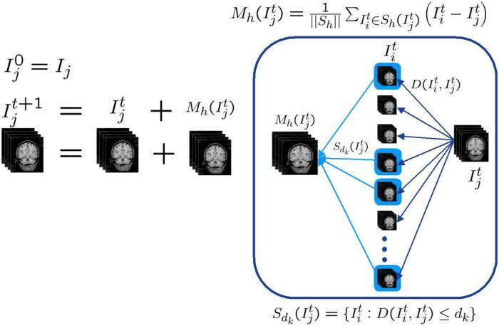
Atlas stratification process. Ij are the initial subjects. At each iteration for each subject j, is calculated from the subject at the tth iteration and the mean shift of the subject, . The process of computing a subject's mean shift is illustrated on the right. The neighborhood is chosen from the kth nearest neighbors forming for update.
The choice of the neighborhood function Sh(Ij) greatly influences the composition of modes. The standard vector norm will drive the modes in different directions than information theoretic measures, overlap metrics, or shape similarity metrics. We have intentionally chosen a loose definition of to allow experimentation with different metrics and measures of similarity. In the following sections we apply two different methods of calculating Sh(Ij), mean squares and mutual information.
In the following sections, we outline eight experiments. Computational burdens have permitted only five of these to be explored in this presentation.
3.2.1 Mean Shift with Mean Square Metric
We consider data that have already been affine transformed to a standard coordinate frame, bias corrected, and delineated with regions of interest for analysis, see Section 4 for details. Here, we eliminate the transformations from the stratification process. This returns us to a standard L2 norm to define the distance between subjects. The neighborhood function is then
| (14) |
where images are treated as column vectors. The update equation is unchanged from (13).
3.2.2 Mean Shift with Mean Square Metric on Stationary PDF
In the derivation of the mean shift algorithm for images, the gradient of the kernel density estimate (4) is estimated from the updated samples, (or for images), yielding the update equation (8). If instead the gradient is estimated from the original samples, the PDF effectively becomes stationary. In this case, the neighborhood function and mean shift become
| (15) |
| (16) |
and are now calculated from the original images Ii rather than . This ensures the estimate of the gradient of the probability density function is taken from the best available data, namely the original samples. Again, we consider delineated regions from image data that have been spatially normalized and bias corrected. The stationary mean shift process is graphically illustrated in Figure 2.
3.2.3 Mean Shift with Mutual Information Metric
Medical images, and MR images in particular, may not repeatably measure the same intensity for the same tissue inter- nor intra-subject. This may result in large distances between subjects even if they are visually similar. Mutual information as used in registration [13,14,15,16] provides a good measure of similarity in this case. While mutual information is not strictly mathematically correct for the mean shift algorithm, it's properties make it interesting for experimentation [17]. The neighborhood function becomes
| (17) |
where is the mutual information between the two images and dk is kth largest mutual information value relative to the image . The update equation remains (13). We again consider delineated images bias corrected, and normalized to a standard space, so no spatial transformation is necessary.
3.2.4 Mean Shift with Mutual Information Metric on Stationary PDF
In this experiment, we replace the norm in the calculation of in (16) with mutual information
| (18) |
where is the mutual information between the two images and dk is kth largest mutual information value relative to the image . The update equation remains (13). As in Section 3.2.3, we consider delineated, bias corrected, and spatially normalized subjects.
3.2.5 Mean Shift and Registration with MI Metric
Delineated, intensity normalized image datasets transformed into a standard space may not always be available. Even if available, the transform to the standardized space may not be the proper transform. If the application demands extremely accurate registration, it may be desirable to register subject images during the stratification process. Incorporating registration into the process is accomplished by modifying the neighborhood function and image update step.
In this experiment, at each iteration t, we align each pair of subjects using Mattes' formulation of mutual information [13] to determine . We used an affine transformation for . The mutual information values for each pair of subjects is denoted . The nearest neighbor set for the mean shift iteration is the set
| (19) |
where dk is kth largest mutual information value relative to the image .
For each mean shift iteration, the pairwise registrations are repeated using and from the previous iteration, producing new transformations and mutual information metric values . At each iteration, we update the samples according to (13), transforming before subtracting
3.2.6 Other Stratification Methods
Many other permutations and combinations of distance metrics, neighborhood functions and updates may be incorporated into the atlas stratification framework. We mention three additional possibilities: the registration experiment in Section 3.2.5 could be repeated with a stationary PDF. Replacing the affine transformation with a B-splines [18] transformation extends the previous experiment to deformable registration (non-stationary and stationary PDF methods could be applied).
4 Data
The data used in our experiments was drawn from two sources: a random selection of 222 MR scans from the High Field MRI Studies of Neurodegenerative Disease conducted at the Albany Medical College's Neuroimaging Center and the freely available Open Access Series of Imaging Studies (OASIS) neuroimaging dataset [19].
The AMC scans were acquired on a 3T scanner (GE Medical Systems, Milwaukee WI). Mean age of the subjects was 74 years and ranged from 55-90 years. The scans were SPGR T1 weighted acquisitions with 15 deg flip angle, 12.1/5.2 TR/TE, 22cm FOV, 2mm slice thickness. In each scan, 96 coronal slices were acquired.
The OASIS dataset consists of a cross-sectional collection of subjects aged 18 to 96. For each subject, 3 or 4 individual T1-weighted MRI scans obtained in single scan sessions are included. The first acquired scan was registered to the Talairach and Tournoux atlas space using a 12 parameter affine transformation, and the remaining scans from the session were registered to the first [20,19]. Scan to scan transforms were composed with the scan to atlas transform, and the scans were resampled to 1 × 1 × 1mm3 in a common coordinate system. For the experiments using this dataset, all images were skull stripped, transformed to a common coordinate system and intensity normalized. The subjects are all right-handed and include both men and women.
5 Multidimensional Scaling
Multidimensional scaling (MDS) is a cluster analysis technique that constructs a low-dimensional representation of a set of high dimensional samples given just the pairwise intersample distances [22,21]. MDS has previously been used in atlas construction by Park et al [2] to identify a subject close to the geometric mean of the population and rooting their atlas on that subject. Here, we use MDS as a qualitative tool to visualize the mean shift clustering process. In the results sections, Figures 5, 7, 9, 11(a) and 13, show the results of MDS applied to inter-subject distances throughout the stratification process. Subjects in the same cluster at the last iteration are labeled with the same symbol. These symbol assignments are propagated back to earlier iterations to illustrate the clustering process. Note that MDS produces a representation unique up to rotation/flip/permutation. Therefore, the visualizations across the iterations or down the bandwidth may vary in configuration by a rotation/flip/permutation. The MDS presentations use either a metric stress or a Sammon [22] criteria depending on which provided a clearer picture of the modes.
Fig. 5.

MDS results for mean shift with mean square metric experiment. The plots show MDS results for iterations 1, 2, 4 and 9 of the algorithm. Colored symbols indicate modes from iteration 9, indicating the evolution of the modes. Five modes were identified containing 72, 216, 46, 28 and 54 subjects.
Fig. 7.

MDS results for iteration 9 of mean shift with mean square metric on stationary PDF (a). In (b) colored symbols indicate subjects corresponding to the modes found by MDS in iteration 9 of the non-stationary experiment (Figure 5). Though not clearly clustered, there is a suggestion of clustering into modes similar to the non–stationary PDF experiment.
Fig. 9.

MDS results of the mean shift with mutual information algorithm. Iterations 1, 2, 4 and 9 are shown. Five modes were identified containing 27, 153, 53, 105 and 78 subjects.
Fig. 11.

MDS results for iteration 9 of mean shift with mutual information on stationary PDF (a). In (b) colored symbols indicate subjects corresponding to the MDS modes from iteration 9 of the non-stationary experiment (Figure 9). Though not clearly clustered, there is a suggestion of clustering into modes similar to the non–stationary PDF experiment.
Fig. 13.
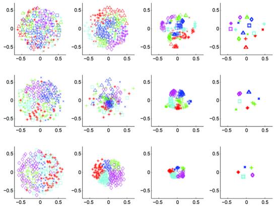
MDS results for mean shift and registration with mutual information metric. The columns show MDS at iterations 1, 2, 4, and 20. The rows illustrate the effect of bandwidth for nearest neighbor sizes 7, 15, and 30. Good convergence is observed for all bandwidths. As expected, MDS shows fewer modes with smaller neighborhoods.
To apply MDS to the results of the mean shift algorithm, we build a dissimilarity matrix which is symmetric with zeros on the diagonals and positive values on the off diagonals. The off diagonal elements are derived from the pairwise distance measures (either mutual information or mean square).
6 Results
For each of the experiments outlined in Section 3.2, we present the evolution of a single subject through the process, MDS results, and visual comparison of the modes. The atlas stratification algorithms were implemented using the Insight Segmentation and Registration Toolkit [23] and command line tools from the AFNI software package [24].
The stratification algorithms of (Sections 3.2.1, 3.2.3, 3.2.2 and 3.2.4) were run on 416 of the OASIS subjects. The AMC data was used for the algorithm of Section 3.2.4. The latter experiment explored the bandwidth and iteration parameter space. The increased numbers of subjects available in the OASIS dataset increased the computation and I/O burden, limiting these experiments to 10 iterations at one bandwidth. The parameter exploration results indicate 10 iterations with a 30 neighbor bandwidth ought to be sufficient to distinguish clusters.
In experiments involving the OASIS subjects, 172 640 (416×415) distance calculations and 416 volume averages of 30 volumes were required at each iteration. This resulted in roughly 7 million volumetric distance calculations. For the AMC dataset, 49 062 (222×221) volume registrations were performed followed by 222 averages of k volumes. The registrations were limited to estimate affine transformations. In total, the processing comprised over 3 million registrations. All processing was distributed over a 500 node compute cluster. Computation time was approximately 4 cpu hours per subject, per iteration.
6.1 Mean Shift with Mean Square Metric
The mean shift with mean square algorithm was run for 10 iterations using 416 subjects from the OASIS dataset. Figure 4 shows axial and coronal images from one randomly chosen subject; original image then iterations 2, 4, and 9. MDS identified 5 modes containing 72, 216, 46, 28 and 54 subjects. Figure 5 shows the mode evolution through iterations 1, 2, 4, and 9. Colored symbols group subjects into modes. In contrast to later experiments, MDS exhibits the behavior of collapsing the modes in one axis. The matrix in Figure 6 shows exemplar subjects from each MDS identified mode on the diagonal. Off-diagonal elements are difference images between the modes displayed with the same contrast settings with mid-gray indicating zero difference. The last two modes appear quite similar.
Fig. 4.

Axial and coronal views of one subject from the mean shift with mean square metric experiment. The original subject image is on the left followed by iterations 2, 4, and 9.
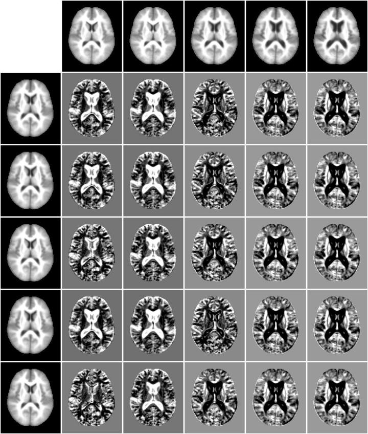
Fig. 6.
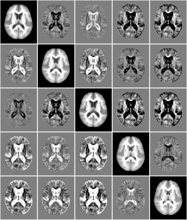
Exemplar subjects from five modes (diagonal images) identified by the mean shift with mean square metric experiment using a bandwidth of 30 neighbors and the difference between these atlases (off-diagonal images). The same contrast settings are used in all difference images with mid-gray indicating zero difference.
6.2 Mean Shift with Mean Square Metric on Stationary PDF
The algorithm of Section 3.2.2 was run for 10 iterations on 416 subjects from the OASIS dataset. MDS results are shown in Figure 7 for iteration 9. MDS failed to identify clear modes in the data. The colored symbols of Figure 7(b) are taken from the non-stationary MDS results and assigned to the same subjects. In this manner, we may compare the modes from the non-stationary experiment to this one. It would appear that several of the modes are clustered together, and have not separated as before. Two modes (green “pluses” and blue “crosses”) appear diffusely mixed. More iterations may be needed to properly identify the modes in the stationary PDF case; for this work, we did not pursue additional iterations.
6.3 Mean Shift with Mutual Information Metric
This experiment explored mean shift using mutual information as described in Section 3.2.3. The algorithm was run with a bandwidth of 30 neighbors for 10 iterations. Figure 8 is the example subject's original image followed by the evolving image at iterations 2, 4, and 9. MDS again identified 5 modes containing 27, 153, 53, 105 and 78 subjects. Figure 9 shows the MDS results for iterations 1, 2, 4, and 9, again with distinct modes identified by colored symbols. The MDS algorithm used to generate these results was a metric stress criteria. It is expected that the different MDS algorithms give differently shaped projections. While MDS identified 5 modes, the first two modes in Figure 10 are very similar. This may indicate the mode (“blue x's”) completely surrounded by a second mode (“green pluses”) should be combined into one mode.
Fig. 8.

Axial and coronal views of one subject from the mean shift with mutual information experiment. The original subject image is on the left followed by iterations 2, 4, and 9.
Fig. 10.
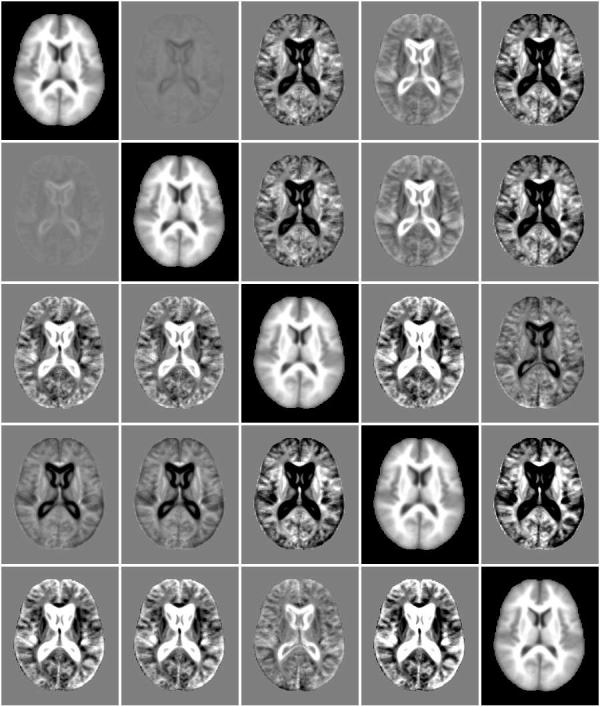
Exemplar subjects from five modes (diagonal images) identified by the mean shift with mutual information experiment using a bandwidth of 30 neighbors. Off-diagonal images are difference between these modes.
A comparison of exemplar subjects from each mode (Figure 10) shows less pronounced differences than mean shift with mean square metric (Figure 6). The first two modes appear quite similar, differing mainly in the region of the ventricles. The modes with enlarged ventricles found with the mean square metric are not present in this experiment. The modes of the two experiments are directly compared in Figure 15.
Fig. 15.
Comparison of the mean shift with mean square metric and mutual information metric. The first row is modes of the mean square metric experiment, the leftmost column are modes from the mutual information experiment. The remaining entries are difference images between modes from the two experiments.
6.4 Mean Shift with Mutual Information Metric on Stationary PDF
We performed ten iterations of the mean shift with mutual information metric on a stationary PDF. As in the previous stationary PDF experiment, MDS did not form distinct clusters (Figure 11). The symbols used for the non-stationary PDF modes were placed on the MDS projection in Figure 11(b), showing potential clustering of the “purple diamonds” on the left. Again, we did not perform additional iterations in this experiment.
6.5 Mean Shift and Registration with Mutual Information Metric
Using this flavor of atlas stratification, twenty iterations were performed on 222 subjects drawn from the AMC subjects using mean shift bandwidths (k) of 7, 15, and 30 neighbors. Figure 12 shows a single subject chosen at random from the k = 30 experiment though different iterations.
Fig. 12.
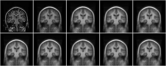
A single subject chosen at random from the mean shift and registration experiment with k = 30. The original subject is shown in the upper left, with iterations 1 through 9 increasing to the right. The remaining iterations are not visibly different.
Figure 13 shows the mean shift algorithm identifies multiple modes in the population. The number of modes being a function of the mean shift bandwidth. For a bandwidth of 30 neighbors, the mean shift algorithm produces 5 clusters containing 33, 39, 43, 47, and 60 subjects. As expected from the kernel density estimation definition in (1), larger bandwidths give fewer modes (as found by MDS).
Figure 14 compares the 5 modes found in the 30 neighborhood bandwidth experiment. The diagonal images are coronal slices of a representative of each mode from Figure 13. Off diagonal entries are difference images of the corresponding modes from the diagonal. Note, the image datasets in this experiment were not skull stripped, nor intensity normalized.
Fig. 14.

Exemplar subjects from modes identified by the mean shift and registration with mutual information metric algorithm (k = 30) are on the diagonal. Difference images are on the off-diagonals.
6.6 Mode Overlap
Given the results of the various experiments, we explore the differences in the modes identified. We compare modes found with mean shift with mean square metric to those found by mean shift with mutual information using Dice similarity coefficients (DSC) [25]. DSC is defined as
where A and B are sets and |A| denotes the cardinality of A. DSC ranges from 0 when sets have a empty intersection to 1 when A == B. The sets used in the DSC calculations are the subject identifiers for the subjects assigned to each mode in each experiment. Several modes in the experiments overlap to some degree as shown in Table 1. Here the columns are the modes identified in the mean shift with mean square metric experiment while rows are modes from mean shift with mutual information metric. The numbers in parenthesis are the size of the mode. The DSC of MS 2 and MI 2, MS 2 and MI 4, and MS 5 and MI 4 indicate a moderate level of overlap in the modes. Exact DSC agreement was not expected due to the different modes found by MS and MI.
Table 1.
Dice Similarity Coefficients for modes identified by Mean Shift with Mean Square Metric (MS) (columns) and Mean Shift with Mutual Information Metric (MI) (rows). The column and row headings indicate the mode from the respective experiment with numbers in parenthesis indicating the mode's cardinality. We consider the sets for DSC to contain the subject identifiers from a mode. The overlap reported is then related to subjects rather than segmentation results as is often reported by DSC.
| Modes | MS 1 (72) | MS 2 (216) | MS 3 (46) | MS 4 (28) | MS 5 (54) |
|---|---|---|---|---|---|
| MI 1 (27) | 0.1818 | 0.1152 | 0.0822 | 0 | 0.0247 |
| MI 2 (153) | 0.2578 | 0.5745 | 0.0704 | 0.0884 | 0.0290 |
| MI 3 (53) | 0.1440 | 0.1041 | 0.2828 | 0.2222 | 0.1308 |
| MI 4 (105) | 0.1808 | 0.0872 | 0.2781 | 0.1654 | 0.5409 |
| MI 5 (78) | 0.1200 | 0.4626 | 0.0161 | 0 | 0 |
Figure 15 visually displays the differences and similarities between modes in the experiments compared in Table 1. The first row displays exemplar subjects from modes found by the mean shift with mean squares metric experiment while the first column displays exemplar subjects from the modes in the mean shift with mutual information experiment. The remaining entries in the figure show the cross-experiment differences in modes.
7 Conclusions
In this paper, we investigate atlas stratification, questioning whether a single atlas is appropriate for a given sample or whether there is evidence from which we can infer multiple atlases, each constructed from a subset of the data. We use the mean shift algorithm to search for modes in the population. If a population has multiple modes, the population should be described by multiple atlases to minimize bias. We have explored only a small portion of the permutations possible with the general atlas stratification framework, considering two different distance metrics, moving and stationary PDFs, and incorporating registration into the framework. Aside from the stationary PDF cases, as the iterations progress, the subjects converge to potential modes of the population. Changes in nearest neighbor measures, stationary vs. non-stationary PDF, update method and bandwidth produce different modes. Further experimentation is required to fully explore the case of stationary PDFs. For practical applications of atlas stratification, the non-stationary approach appears to converge more rapidly than the stationary method.
In the usual course of atlas construction the transformation between a subject and the constructed atlas is preserved. It is possible to maintain the relationship between the original data and the final mode in atlas stratification, however, the purpose of this initial work is to find the modes in the population. As we seek the modes of the distribution, modification of the original samples is necessary. In principle, the outlined approach could be used to identify subjects belonging to each mode for input into arbitrary construction methods. However, we feel the distance metric used for atlas stratification should be linked to the atlas construction method.
While the approach taken here is direct, it is not the only possible construction. For instance, the distance metric does not have to be based on mean squares or mutual information. Overlap metrics or shape similarity metrics on presegmented structures could also be used in this mean shift framework. While our studies were based on an affine transform between subjects, higher order transformations and deformable registrations could be used. Mean shift formulations other than the nearest neighbor variant could also be used.
Aside from the above refinements, we've identified three areas of future research for atlas stratification. The first is a study of the algorithm itself, quantifying the differences between the atlases produced by atlas stratification. The second is a study of the algorithm in context, quantify an improvement in an atlas-based technique when multiple atlases are available. This will require a method to select the most appropriate atlas for a particular subject [26,27]. A final study would involve finding correlations between clinical data and the modes discovered by atlas stratification.
8 Acknowledgments
We would like to note our appreciation for the considerable efforts in collecting and managing the imagery used in this paper. Dr. John Schenck from GE Research and Dr. Earl Zimmerman from the Albany Medical College co-directed the collaboration on High Field MRI Studies of Neurodegenerative Disease as well as recruited volunteers for the study. Dave Henderson from GE Research provided data management and John Cowan from the Albany Medical College performed the subject scans. We are indebted to Dr. Randy Buckner for making the OASIS datasets available and for the gracious support by Dr. Daniel Marcus of Washington University. This work is part of the National Alliance for Medical Image Computing (NAMIC), funded by the National Institutes of Health through the NIH Roadmap for Medical Research, Grant U54 EB005149.
Footnotes
Publisher's Disclaimer: This is a PDF file of an unedited manuscript that has been accepted for publication. As a service to our customers we are providing this early version of the manuscript. The manuscript will undergo copyediting, typesetting, and review of the resulting proof before it is published in its final citable form. Please note that during the production process errors may be discovered which could affect the content, and all legal disclaimers that apply to the journal pertain.
This work is part of the National Alliance for Medical Image Computing (NAMIC), funded by the National Institutes of Health through the NIH Roadmap for Medical Research, Grant U54 EB005149. Information on the National Centers for Biomedical Computing can be obtained from http://nihroadmap.nih.gov/bioinformatics.
References
- 1.Marsland S, Twining C, Taylor C. Groupwise non-rigid registration using polyharmonic clamped-plate splines. MICCAI. 2003:771–779. [Google Scholar]
- 2.Park H, Bland P, Hero A, Meyer C. Least biased target selection in probabilistic atlas construction. MICCAI. 2005:419–426. doi: 10.1007/11566489_52. [DOI] [PubMed] [Google Scholar]
- 3.Studholme C, Cardenas V. A template free approach to volumetric spatial normalization of brain anatomy. Pattern Recogn. Lett. 2004;25(10):1191–1202. [Google Scholar]
- 4.Bhatia K, Hajnal J, Puri B, Edwards A, Rueckert D. Consistent groupwise non-rigid registration for atlas construction. ISBI. 2004:908–911. [Google Scholar]
- 5.Craene MD, du Bois d'Aische A, Macq B, Warfield S. Multi-subject registration for unbiased statistical atlas construction. MICCAI. 2004:655–662. [Google Scholar]
- 6.Lorenzen P, Davis B, Joshi S. Unbiased atlas formation via large deformations metric mapping. MICCAI. 2005:411–418. doi: 10.1007/11566489_51. [DOI] [PubMed] [Google Scholar]
- 7.Zollei L, Learned-Miller E, Grimson E, Wells W. Efficient population registration of 3d data. ICCV. 2005 2005. [Google Scholar]
- 8.Fukunaga K, Hostetler L. The estimation of the gradient of a density function with applications in pattern recognition. T-IT. 1975;21(1):32–40. [Google Scholar]
- 9.Cheng Y. Mean shift, mode seeking and clustering. IEEE Transactions on Pattern Analysis and Machine Intellegence. 1995;17(8):790–799. [Google Scholar]
- 10.Comaniciu D, Meer P. Mean shift: A robust approach toward featue space analysis. IEEE Transactions on Pattern Analysis and Machine Intellegence. 2002;24(5):603–619. [Google Scholar]
- 11.Comaniciu D, Ramesh V, Meer P. Real-time tracking of non-rigid objects using mean shift. CVPR. 2000;2:142–149. 2000. [Google Scholar]
- 12.Silverman B. Density estimation for statistics and data analysis. Chapman and Hill; 1992. [Google Scholar]
- 13.Mattes D, Haynor D, Vesselle H, Lewellen T, Eubank W. PET-CT image registration in the chest using free-form deformations. IEEE Transactions on Medical Imaging. 2003;22(1):120–128. doi: 10.1109/TMI.2003.809072. [DOI] [PubMed] [Google Scholar]
- 14.Wells W, Viola P, Atsumi H, Nakajima S, Kikinis R. Multi-modal volume registration by maximization of mutual information. Medical Image Analysis. 1996;1(1):35–51. doi: 10.1016/s1361-8415(01)80004-9. [DOI] [PubMed] [Google Scholar]
- 15.Collignon A, Maes F, Delaere D, Vandermeulen D, Suetens P, Marchal G. Automated multimodality medical image registration using information theory; Proc. 14th Int. Conf. Information Processing in Medical Imaging; Computational Imaging and Vision 3; 1995. pp. 263–274. [Google Scholar]
- 16.Maes F, Collignon A, Vandermeulen D, Marchal G, Suetens P. Multimodality image registration by maximization of mutual information. IEEE Transactions on Medical Imaging. 1997;16(2):187–198. doi: 10.1109/42.563664. [DOI] [PubMed] [Google Scholar]
- 17.Zöllei L, Jenkinson M, Timoner S, Wells W. A marginalized MAP approach and EM optimization for pair-wise registration; International Conference on Information Processing in Medical Imaging; 2007. [DOI] [PMC free article] [PubMed] [Google Scholar]
- 18.Rueckert D, Frangi AF, Schnabel JA. Automatic construction of 3-D statistical deformation models of the brain using nonrigid registration. IEEE Transactions on Medical Imaging. 2003;22(8):1014–1025. doi: 10.1109/TMI.2003.815865. [DOI] [PubMed] [Google Scholar]
- 19.Marcus D, Wang T, Parker J, Olsen T, Ramaratnam M, Csernansky J, Morris J, Buckner R. Open access structural imaging series (OASIS): Cross-sectional data across the adult lifespan. J. Cog. Neurosci. In Press. [Google Scholar]
- 20.Buckner R, Head D, Parker J, Fotenos A, Marcus D, Morris J, Snyder A. A unified approach for morphometric and functional data analysis in young, old, and demented adults using automated atlas-based head size normalization: reliability and validation against manual measurement of total intracranial volume. Neuroimage. 2004;23:724–738. doi: 10.1016/j.neuroimage.2004.06.018. [DOI] [PubMed] [Google Scholar]
- 21.Everitt B, Landau S, Leese M. Cluster Analysis. Arnold; 2001. [Google Scholar]
- 22.Sammon JW., Jr. A nonlinear mapping for data structure analysis. IEEE Transactions on Computers. 1969;18(5):401–409. [Google Scholar]
- 23.Ibanez L, Schroeder W, Ng L, Cates J. The ITK Software Guide. 2nd Edition. Kitware, Inc.; 2005. (ISBN 1-930934-15-7). http://www.itk.org/ItkSoftwareGuide.pdf. [Google Scholar]
- 24.Cox R, Hyde J. Software tools for analysis and visualization of FMRI data. NMR in Biomedicine. 1997;10:171–178. doi: 10.1002/(sici)1099-1492(199706/08)10:4/5<171::aid-nbm453>3.0.co;2-l. [DOI] [PubMed] [Google Scholar]
- 25.Dice L. Measures of the amount of ecologic association between species. Ecology. 1945;26:297–302. [Google Scholar]
- 26.Koikkalainen J, Lötjönen J. Model library for deformable model-based segmentation of 3-D brain MR-images. MICCAI. 2004:540–547. [Google Scholar]
- 27.Rohlfing T, Brandt R, Menzel R. Evaluation of atlas selection strategies for atlas-based image segmentation with application to confocal microscopy images of bee brains. NeuroImage. 2004;21:1428–1442. doi: 10.1016/j.neuroimage.2003.11.010. C. R. M. Jr. [DOI] [PubMed] [Google Scholar]