A Three Dimensional Model of the Feline Hindlimb

Abstract

This paper describes a three dimensional musculoskeletal model of the feline hindlimb based on digitized musculoskeletal anatomy. The model consists of seven degrees of freedom: three at the hip and two each at the knee and ankle. Lines of action and via points for 32 major muscles of the limb are described. Interspecimen variability of muscle paths was surprisingly low: most via points displayed a scatter of only a few millimeters. Joint axes identified by mechanical techniques as non-coincident and non-orthogonal were further honed to yield moment arms consistent with previous reports. Interspecimen variability in joint axes was greater than that of muscle paths and highlights the importance of joint axes in kinematic models. The contribution of specific muscles to the direction of endpoint force generation is discussed.

The production of coordinated movement requires that the nervous system control muscle forces to generate joint torques required for control of the limb endpoint in Euclidean space. The nervous system must be capable of transformation between Euclidean space and joint space and between joint space and muscle space to determine what set of muscle activations is required to generate a desired motion (Lacquaniti and Maioli, 1994). Knowledge of these transformations is required to understand the basis of locomotion (Prochazka, 1996; Rossignol, 1996; Zernicke and Smith, 1996; Duysens et al., 2000; Stein et al., 2000) and other forms of voluntary movement (Mussa-Ivaldi et al., 1985; Flash, 1987; Feldman and Levin, 1995; Ghez et al., 1995; Gordon et al., 1995; Gottlieb et al., 1997; Kargo and Giszter, 2000; Ting et al., 2000).

These transformations are based on the architecture and mechanics of the musculoskeletal system. Details of this information are available for humans (Delp et al., 2001), non-human primates (Cheng and Scott, 2000) and other animals, (Kargo et al., 2002; Kargo and Rome, 2002). The cat has been an important experimental subject for studies of normal and abnormal motor control (Macpherson, 1988; Pratt and Loeb, 1991; Prochazka, 1996; Rossignol, 1996; Macpherson and Fung, 1999), but detailed architectural information is not available in comprehensive form. The goal of this paper is to report our studies of the musculoskeletal anatomy of the feline hindlimb and a corresponding mathematical model to predict the transformations described above.

Perhaps the first issue that arises in the construction of such a model is interspecimen variability. To generalize from one or a few measurements to a stereotypical or canonical anatomy, the variation between specimens must be small. If interspecimen variation is large, then the description of a sample is less likely to be representative of any individual. Interspecimen variability may also offer a means to understand the observed inter-individual variation in motor control patterns (McCollum et al., 1995).

Another concern is the choice of kinematic constraints to be imposed on the model. These have previously ranged from simple hinges in anatomical planes (Mussa-Ivaldi et al., 1985) to screw-displacement axes (Woltring et al., 1985). The former is computationally straightforward, but practically limited. The latter is most useful in describing a specific observed motion for inverse dynamics, and either may introduce non-physiological constraints on the system. A compromise between these extremes has been suggested (Hollister et al., 1992), in which a joint is approximated as a combination of hinges representing physiological planes defined by joint morphology, rather than anatomical planes defined by body posture. This approach allows the computational simplicity of single degree-of-freedom joints, and extends the range over which that approximation closely represents the actual motion.

The purpose of the work presented in this paper was to construct a three dimensional model of the feline hindlimb. Specific attention is focused on interspecimen variation in muscle paths and the use of joint axes.

MATERIALS AND METHODS

Hindlimbs were harvested from five cats (weight 3.5±0.5kg) sacrificed during the course of experiments not disturbing the limb anatomy. Limbs were collected with pelvis and lumbar vertebrae intact to preserve hip musculature and psoas minor origin. Two 6 mm self-tapping, stainless steel threaded rods were driven through both femur and tibia, and 3 mm rods were driven through the calcaneus and distal tarsals.

Mechanical Axis Identification

Motion of the limb segment is constrained by bone, ligament and other tissues, which reduces the degrees of freedom between adjacent segments. Motion at the knee and ankle was described using two rotational degrees of freedom at each joint, and these axes were determined in four of the five specimens.

A mechanical system or ‘axis finder,’ similar to that described by Hollister et al. (1993), was used to identify the axes of rotation (Fig. 1). One limb segment was fixed to the laboratory bench by threaded pins driven through the bone. To the segment on the other side of the joint was fixed a rail, also by a pair of transcortical pins. A guide holder was mounted on this rail using a clamp that allowed sliding and rotation of the guide holder relative to the rail. A hollow guide tube was mounted at the end of the guide holder by a ball and socket joint. By changing the clamp position, it was possible to place the guide holder at any location relative to the fixed segment, and the ball-and-socket joint allowed the guide tube to be oriented at any direction to the fixed segment. While the joint was manually articulated, the position and orientation of the guide tube were manipulated to minimize the motion of the tube relative to the fixed segment. When the guide tube is not aligned with the axis of rotation, its free end sweeps an arc as the floating segment is moved, and minimization of this motion indicated alignment of the tube with the hinge axis. A hole was then drilled through the fixed segment, using the hollow tube as a guide, and a pin inserted along the joint axis.

Fig. 1.

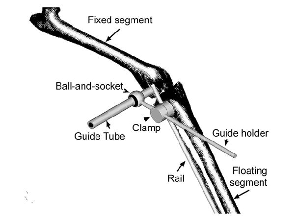
The device used for mechanical identification of joint axes. A rail was fixed to one limb segment by bone screws, and the guide holder could be freely positioned using a sliding, rotating clamp. The guide tube, fixed to the guide holder by a ball-and-socket joint was able to be arbitrarily oriented to the joint. Proper identification of the axis was indicated when the rail attached segment could be freely rotated without moving the guide tube.

This procedure depends strongly on the ability of the experimenter to ‘feel’ the joint motion, which requires some skill and practice. The technique has been used successfully in other, similar joint systems (Hollister et al., 1992, 1993) and was considered a sufficient technique for determining the approximate center of rotation. The intention of this work was less to replicate the exact anatomy and function of a particular specimen than to generate a model that balanced anatomical complexity and computational simplicity.

Digitization of muscle points

Following identification of two axes at the knee and one at the ankle, the limb was immobilized in a stance-like posture using a system of clamps. The hip was held at approximately 90°, the knee at 100° and the ankle at 110° (Fig, 2). The limb was then bathed in 4% paraformaldehyde in phosphate buffered saline (PBS) for 1-2 weeks. After this fixation, the limb was transferred to a PBS bath. The immobilization frame was left in place during muscle point recording.

Fig. 2.

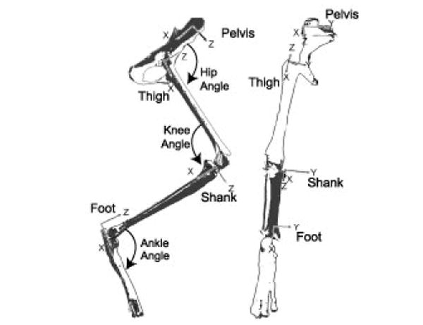
Conventions used for segmental reference frames and joint angle descriptions.

Muscle point recording for each specimen was performed over the course of several weeks, with the limb being stored in PBS at 4°C between measurements. Each point was digitized on at least three separate sessions. Each digitization session followed a similar pattern. The limb would be mounted within the workspace of a Cartesian frame. The custom built frame consisted of 3 mutually perpendicular, graduated bars connected by vernier-scale stereotaxic clamps. The X-axis was mounted to the laboratory bench; the vertical Z axis was held to the X axis using the clamp from a stereotaxic electrode holder (Kopf Instruments, Tujunga, CA), and supported the Y-Axis by a similar clamp. A stylus, fixed to the end of the Y axis, was positioned at each muscle origin, insertion and via point, and its location recorded. The vernier scale clamps were readable to 0.1 mm, and repeated measurements of calibration points indicate that this system has a reproducibility of ±0.2mm. Each muscle follows a unique path between origin and insertion. In many cases, this was a reasonably undistorted, straight line. In those cases, such as soleus, only muscle origin and insertion were recorded. In cases where the path of a muscle makes a distinct change in direction, as tibialis anterior at the crural ligament, or semitendinosus around the belly of the gastrocnemius, and the location of these intermediate via points was also recorded. In addition to muscle points, reference points on the immobilization frame were recorded to permit registration of successive measurements.

Points were digitized in 5-6 layers from 2 faces. The more superficial layers were typically recorded from medial and lateral aspects, while cranial and caudal aspects were more efficient for the deeper layers. After at least 3 recordings of each point on a muscle, the muscle was carefully removed to expose the deeper tissue.

Segment reference frames

Bony landmarks were used to define segmental reference frames (Table 1, Fig. 2). These points were chosen to define the long X axis and X-Y plane. The pelvis was defined by the ipsilateral iliac crest and ischial tuberosity and contralateral iliac crest. The thigh was defined by the femoral greater trochanter, lateral and medial femoral epicondyles. The shank was defined by the medial tibial condyle and the lateral and medial malleoli. The foot was defined by the end of the calcaneus, and the 2nd and 5th metatarsal-phalangeal joints.

Table 1.

Definitions of segmental coordinates

Segment	Origin	X-direction	Y-direction
Pelvis	Ipsilateral iliac crest	Ipsilateral ischial tuberosity	Contralateral iliac crest
Thigh	Greater trochanter	Lateral femoral condyle	Medial femoral condyle
Shank	Medial tibial epicondyle	Medial malleolus	Opposite to lateral malleolus
Foot	Calcaneus	Bisect Medial and Lateral metatarsal-phalangeal joints	Medial metatarsal-phalangeal joint

In each case, the X axis was defined to lie exactly along the digitized points. The Z axis was then defined by the cross product of the X-axis with the Y-directed third reference point. Finally, the Y-axis was determined by crossing the Z-axis with the X-axis. This approach yielded orthogonal axes for each segment with X positive towards the distal end of the segment, Y positive medially, and Z positive cranially. Coordinates for the single left limb were reflected across the X-Z plane.

Coordinate transformation

It was not practical to place the limb in a globally reproducible position and orientation for each of the repeated measurement sequences, so a procedure was developed to transform the data, or record set, generated by each measurement sequence for a particular specimen to a common reference frame. An initial set of measurements was made that contained as many frame-fixed reference points as possible for each specimen. Subsequent record sets contained a subset of these calibration points, and each of the muscle points that was accessible to the measurement stylus in a particular orientation of the specimen at a particular stage of dissection. A typical specimen yielded 70-100 such record sets. Each of these record sets was converted to the coordinate system defined by the initial measurement of reference points (C₀). Reference points common to both record sets were broken into groups of 3 and used to define orthonormal coordinate frames. A translation and rotation that mapped the measured data points (D₁) onto C₀ is then given by

$$D_0=X_0^T{X}_1(D_1-\mathbf{T})$$

where X₀ are the components of the reference frame in C₀, X₁ are the components of the reference frame in the coordinates to be converted, and T the displacement from the origin of X₀ to X₁.

There were typically 6-10 reference points in common between measurement sets, giving 50-200 groups of 3 points and estimates for X₁, X₀ and T. These estimates were averaged and re-normalized to yield the final conversion parameters. This approach was taken to minimize the impact of error associated with measurement of the reference points.

Statistics

All data were normalized to a tibial length of 11.1cm, the mean for these specimens. Unless otherwise noted, numerical values are reported as mean±S.D.

Model definition

The normalized data were used to define a six segment model in DADS 9.5 (LMS/CADSI, Coralville, IA). In addition to the four anatomical segments, an additional phantom segment was required at the knee and ankle to join the sagittal and non-sagittal axes. An ancillary set of coordinate systems (DADS CSYS elements) was defined, aligned with each joint. These CSYSs simplified the process of manipulating the limb by permitting direct reorientation of each joint, in its own coordinates, eliminating the need to recalculate the position and orientation of each segment.

Each specimen was fixed in a slightly different posture, resulting in a slightly different estimate for each joint position in its proximal and distal segments. To mediate these differences, the distal segment was moved to align the origin of the sagittal axis, and the axis was reoriented to the mean of the proximal and distal estimates. The flexion axis was chosen as the alignment point because of the higher reproducibility and confidence in these axes.

Flexion axes were determined by an iterative process. Due to the uncertainties associated with the mechanical axis identification procedure, the identified axes were used as a starting estimate, which was further refined by comparison of the model moment arms with previously reported results (Young et al., 1993). The manual adjustment of axis location allowed the axes to be chosen to represent the greatest range of available data. Results for both the unadjusted average and the finalized axis are reported. Modifications consisted primarily of altering the location of the axis, with minimal manipulation of axis orientation.

The nonsagittal knee axis was derived from the mean of the three most similar estimates. Its origin was the translated, along its axis, to minimize its distance from the sagittal axis. This was a purely cosmetic alteration, as the kinematic constraint is independent of its “point” origin.

The estimates for the nonsagittal ankle axes, derived from rotation of the reference frame, varied widely. Two of these estimates were in similar directions and those two were used to define the axis orientation. Using this axis orientation, the position of the axis was initially estimated from those two measurements and refined by repeated comparison with moment arms reported by Young et al. (1993) and the torque vectors reported by Lawrence and coworkers (1993).

Muscle length changes were defined by the two contact points spanning each joint. Segments were modeled as rigid bodies, so the length of any muscle section entirely contained within a single body segment never changed. Muscle architecture was taken from Roy et al., (1998) and Sacks and Roy (1982), and muscles were assumed to be at 95% optimal length (L₀) in the stance configuration (Burkholder and Lieber, 2001).

Model validation

To evaluate the accuracy of the model, predicted moment arms were compared with those reported by Young and colleagues (1993) and with the torque vectors reported by Lawrence and coworkers (1993). This test is somewhat artificial, as these data were also used to establish the final position and orientation of the axes. Because joint axes were not aligned with anatomical axes, moment arms were evaluated by a regression procedure. The anatomical orientation--flexion, adduction, and inversion -- of the distal segment was calculated over a range of mechanical joint configurations. Muscle lengths were determined over the same range of joint configurations, and fit by linear regression to 3^rd order polynomial functions of the calculated anatomical orientation. Partial derivatives of these polynomials with respect to the anatomical axes are the effective moment arms (An et al., 1984).

As a second validation of the model, endpoint forces produced by individual muscles were estimated. With the cat model in its starting configuration, force was applied through each muscle, while keeping the configuration of the limb constant. The femur was fixed in space for these calculations, so the contribution of effects related to hip torques is suppressed. Endpoint force resultants were normalized to the applied muscle force. The model predictions were compared to the results of analogous experiments (Nichols, et al., 2003). Briefly, the toe of a decerebrate cat was fixed to an ATI 6-degree-of-freedom force transducer (ATI Gamma). A background level of force was established by activation of the crossed-extension reflex, and individual muscles were stimulated for 20 ms at 200 Hz by indwelling fine wire electrodes. The change in force elicited by the intramuscular stimulation was compared with the model predicted change in force.

RESULTS

The mechanical axis identification approach yielded generally consistent orientations and positions for the three axes and four specimens on which it was used. Axes for the final model were chosen based on confidence in particular axis measurements and comparison of muscle moment arms with published values (Young et al., 1993; Lawrence et al., 1993). Both the raw averages and the adjusted, final axes as incorporated in the model are reported in Table 1.

For the knee flexion axis (Fig. 3), three estimates are within 10° of each other in direction and 2.4mm in position of each other. One apparent outlier was found to diverge from the remaining 3 by more than 40° and was excluded from the averages. The ankle flexion axis (Fig. 4) shows similar scatter of 15° and 2.9 mm. The knee rotation axis, which accounts for the abduction-internal rotation motion, shows noticeably more variability (Fig. 4). This variability may be attributed to the technical difficulty of drilling into the tibia at a shallow angle.

Fig. 3.

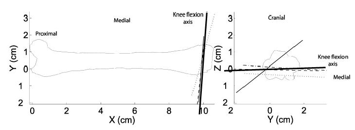
Knee flexion axis estimates for each specimen are presented as thin lines with the axis used in the final model presented as a heavy line. The final axis discards the single wild estimate and is slightly reoriented to match the tibial estimate.

Fig. 4.

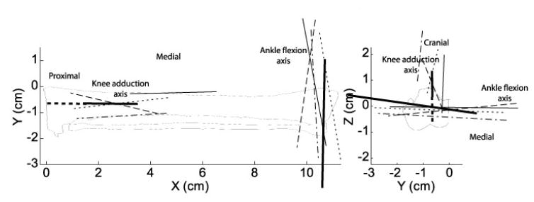
Thin lines represent the axes of rotation of the shank for each specimen, and the axes used in the model are shown as heavy lines. The steep inclination of the proximal axis reflects the strong coupling of abduction and internal rotation at the knee.

The ankle rotation axis was only identified by reference frame rotation and not by the mechanical system used for the other motions. This already coarse technique was further hampered by the limited range of non-sagittal motion at the ankle, giving rise to large between-subjects variation. The measurements of this axis were used only as a guide in choosing the final position and orientation, with previously published reports of muscle moment arms (Young et al., 1993) and joint torques (Lawrence and Nichols, 1999) used as refining guides.

Segmental data showed surprisingly little variation across specimens (Tables 3-6). Those points that did show unusually large variability were generally associated with muscles with broad, distributed insertions, such as the biceps femoris. These distributed connections were digitized as single points, so this variability reflects both the actual anatomical variability and the variability of the experimenter’s estimate of the centroid of the connection. The standard deviations reported here thus reflect the variance in point location, the size of the “point” being measured, and its distance from the coordinate defining points. The volume of these standard deviation ellipsoids ranges from 0.18 cm³ for the tibialis anterior insertion to over 175 cm³ for the gluteus maximus origin. In general, though, the discrete points fell within a volume of less than 1 cm³.

Table 3.

Location of femoral points.

Point	X (cm)	Y (cm)	Z (cm)
Adductor femoris insertion	5.36±2.24	0.39±0.15	0.15±0.37
Adductor longus insertion	4.94±0.49	0.87±0.62	0.17±0.44
Biceps femoris, anterior head insertion	10.52±0.66	0.27±0.42	-1.56±2.24
Biceps femoris, anterior head, via point	9.28±0.98	0.02±0.07	0.37±0.11
Caudofemoralis insertion	8.62±1.14	-0.04±0.28	0.47±0.24
Extensor digitorum longus origin	10.16±0.31	0.16±0.18	0.26±0.62
Femoral head	0.20±0.37	2.16±1.05	0.16±0.28
Gluteus maximus insertion	-0.22±0.49	-0.18±0.37	0.27±1.09
Gluteus medius insertion	0.23±0.87	-0.42±0.25	-0.08±0.30
Gluteus minimus insertion	0.10±0.76	-0.25±0.26	0.76±0.65
Greater trochanter	0.00	0.00	0.00
Iliopsoas insertion	0.81±0.50	1.11±0.88	-0.02±0.67
Lateral femoral condyle	9.62±0.30	0.00	0.00
Lateral gastrocnemius origin	9.11±0.23	-0.05±0.12	0.26±0.51
Medial femoral condyle	9.80±0.81	1.74±0.52	0.00
Medial gastrocnemius origin	9.15±0.36	1.15±0.12	0.06±0.52
Pectineus insertion	3.72±0.40	0.79±1.10	-0.09±0.38
Plantaris origin	9.05±0.22	-0.19±0.43	0.27±0.51
Psoas minor insertion	0.90	1.21	0.69
Pyriformis insertion	0.13±0.60	0.18±0.14	0.08±0.12
Quadratus femoris insertion	0.78±0.21	0.63±0.20	-0.54±0.16
Rectus femoris via point	9.98±0.46	0.80±0.22	1.50±0.37
Semimembranosus insertion	9.97±0.36	1.38±0.34	-0.01±0.79
Vastus intermedius origin	1.93±0.41	0.41±0.43	0.43±0.17
Vastus intermedius via point	9.84±0.60	0.59±0.58	1.33±0.32
Vastus lateralis origin	0.50±0.34	-0.04±0.56	0.20±0.35
Vastus lateralis via point	9.78±0.38	0.39±0.62	1.30±0.26
Vastus medius origin	1.70±0.52	1.10±0.87	0.38±0.47
Vastus medius via point	10.06±0.30	1.15±0.27	1.05±0.53

Table 6.

Knee and ankle moment arms at stance configuration.

Muscle	Knee Extension (cm)	Knee External(cm)	Ankle Flexion (cm)	Ankle Abduction(cm)	Ankle Flexion (Literature)
BFP	-2.78	-1.96
EDL	0.27	0.27	1.09	-.32	1.23
FDL			-.22	-.85	-0.18
FHL			-.23	.083	-0.57
GRAC	-2.82	1.10
LG	-0.88	1.18	-1.50	.095	-1.6
MG	-0.86	-0.06	-1.57	.22	-1.6
PB			-.02	.56	-0.03
PLAN	-0.94	1.33	-1.55	.093	-1.6
PL			.21	.57	0.37
PT			.18	.38	-0.03
RF	1.05	-0.57
SM	-0.67	1.22
SOL			-1.35	.09	-1.6
ST	-3.65	0.82
TA			1.50	-.01	1.20
TP			.05	-.93	-0.04
VI	0.98	-0.83
VL	0.95	-1.05
VM	0.98	-0.11

Literature knee estimates are taken from Young et al. (1993). BFP, biceps femoris posterior; EDL extensor digitorum longus; FDL, flexor digitorum longus; FHL, flexor hallucis longus; GRAC, gracilis; LG, lateral gastrocnemius; MG, medial gastrocnemius; PB, peroneus brevis; PLAN, plantaris; PL, peroneus longus; PT, peroneus tertius; RF, rectus femoris; SM, semimembranosus; SOL, soleus; ST, semitendinosus; TA, tibialis anterior; TP, tibialis posterior; VI, vastus intermedius; VL, vastus lateralis; VM, vastus medialis.

Specimen variability

The reproducibility of measurement of an individual muscle point depended strongly on its identity. Measurements associated with broad or distributed muscle attachments, such as the adductor femoris insertion, which displayed a spatial variability of 2.3 cm, were more variable than points associated with discrete attachments, such as tibialis anterior insertion, which varied by only 0.6 cm or about the area of its tendon. Individual specimens spanned a mass range of 3.0-4.3 kg, and tibia lengths ranged from 9.81 cm to 11.98 cm. Although measurements in individual specimens were normalized to a tibia length of 11.1 cm, it was expected that this large size range would result in substantial inter-specimen variability. Overall, variability was similar within and between specimens. The spatial variance of each point was calculated as the sum, in quadrature, of the standard deviation of each dimension of that point. When this variation was calculated for each point for each specimen, intra-specimen variability was found to be 0.49 cm, as compared with 0.51 cm between specimens. Reproducibility of measurements during measurement calibration was 0.02 cm. This suggests that the greatest source of variation in the measurement process is the ability of an individual experimenter to identify a consistent point.

Moment arms

Moment arms calculated from segmental motion and muscle excursion were similar to those reported in the literature (Table 6). The variation of moment arm with joint angle was also similar to that reported for selected ankle-crossing muscles (Figs. 5 and 6). As noted by Young et al. (1993), many of these muscles display abduction moment arms that cross zero, indicating intrinsic mechanical stability. Notable deviations between the present model and existing data include peroneus tertius (PT), which was found to have a flexor moment in the stance configuration, in comparison with a negligible, but extensor moment reported in the literature, and a similar reversal of tibialis posterior (TP). The major action of these muscles is out of the sagittal plane, and we report a 0.38 cm abduction moment arm for PT and a 0.93 adduction moment arm for TP that compare with 0.41 cm and 0.68 cm, respectively (Young et al., 1993).

Fig. 5.

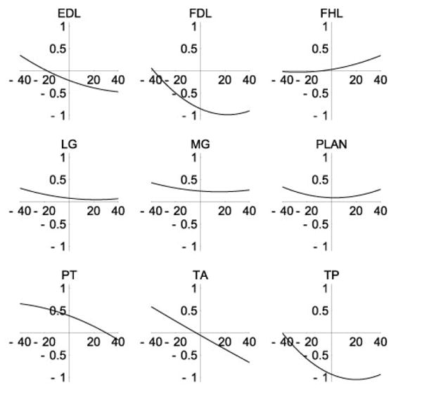
Ankle abduction moment arms (cm). Moment arms and angles(°) are positive in abduction.

Fig. 6.

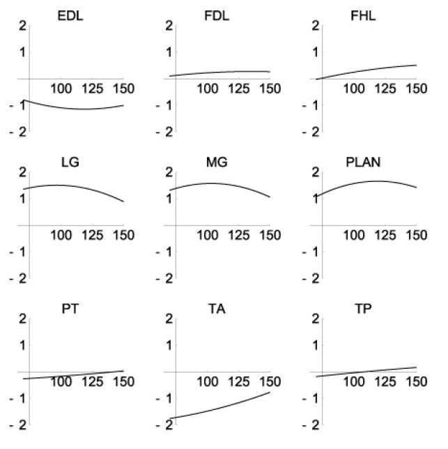
Ankle extension moment arms(cm). Moment arms and angles (°) are positive in extension.

Endpoint forces

Forces generated by individual muscles at the endpoint strongly reflected the kinematic constraints placed on the limb. Resultants were generally clustered along two axes in the horizontal plane: one axis predominantly anterior-posterior (Fig. 7), and the other roughly perpendicular. Muscles generating predominantly lateral forces were flexor digitorum longus(FDL), peroneus brevis (PB), peroneus longus (PL), peroneus tertius (PT) and tibialis posterior (TP), which are typically considered ankle stabilizers. In the parasagittal plane, forces were concentrated along an axis associated with ankle flexion and inclined approximately 60° from horizontal or along an axis associated with knee flexion, declined approximately 70° from horizontal. Muscles with a strong knee extension moment were found to generate forces directed down and cranially, where muscles with a strong ankle extension moment generated forces directed down and caudally. Based on the direction of endpoint force resultant, the muscles of the lower limb could be separated into six groups: extensor digitorum longus (EDL) and tibialis anterior (TA), lifting the foot with an anteriorly directed component, or rotating counterclockwise; biceps femoris (BF), gracilis and semitendinosus (ST), lifting the foot with a posterior component, or retracting the limb; rectus femoris (RF), vastus intermedius (VI), vastus lateralis (VL) and vastus medialis (VM) supporting weight and directed anteriorly, or extending the limb; flexor hallucis longus (FHL), lateral gastrocnemius (LG), medial gastrocnemius (MG), plantaris and soleus supporting weight and directed posteriorly, or rotating counterclockwise; PB and PL generating lateral force; and FDL, PT and TP generating medially directed force.

Fig. 7.

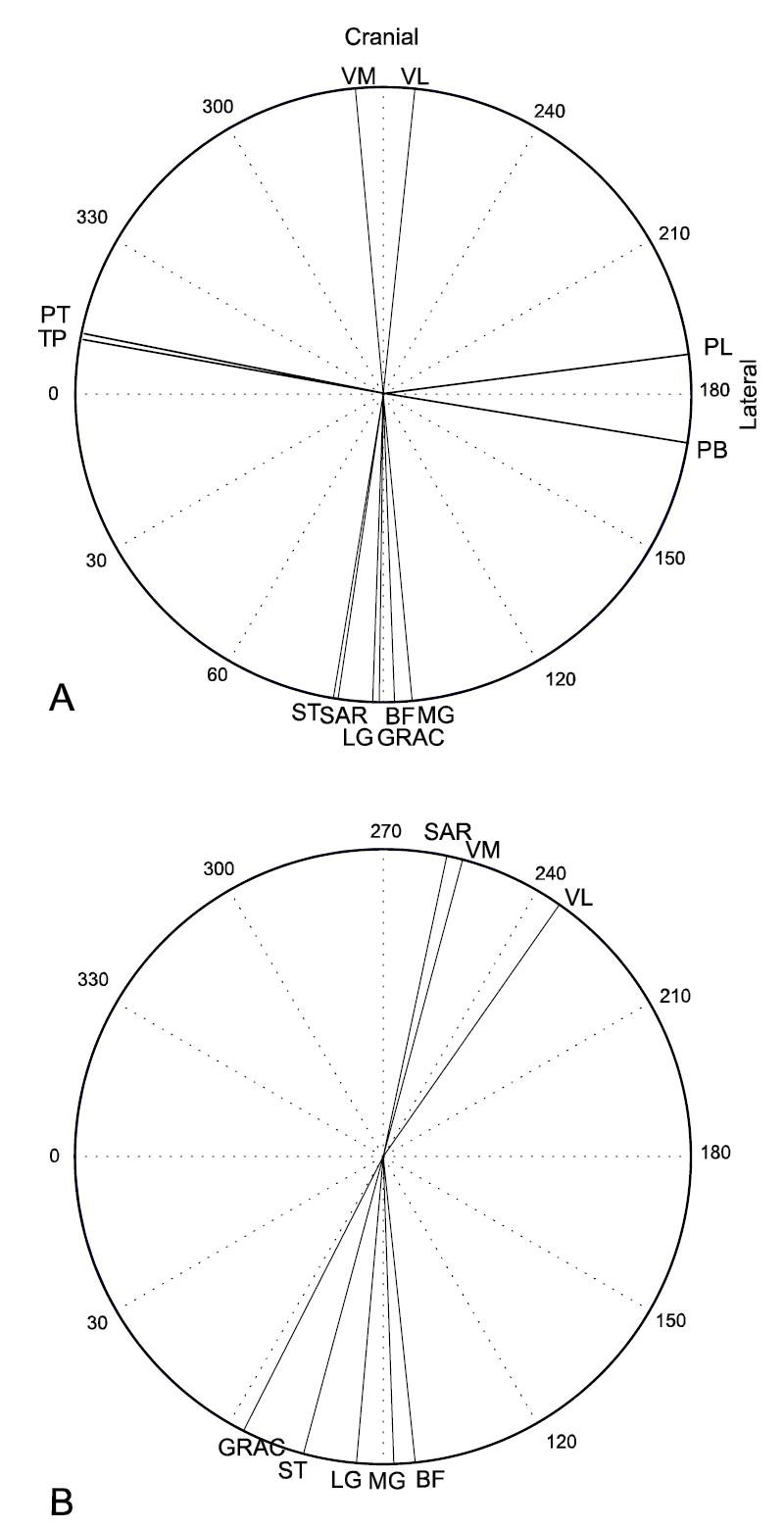
Horizontal plane endpoint forces predicted by the model (A), or generated by intramuscular stimulation of individual muscles (B, Nichols et al., 2003). Although force directions appear to be rotated between the two cases, the relative orientations of most muscles are maintained.

Model predicted endpoint force directions were comparable (Fig. 7) to those measured experimentally (Nichols et al., 2003). Predicted force directions were more closely clustered along the cranial-caudal axis than were experimental results, but the relative orientation of muscle resultants was similar. For example, the model predicted that ST would be more medially directed than is LG, and that LG would be more medially directed than is MG, a relationship that was observed in the experimental results. Notable points of divergence include sartorius, which the model predicts to be a knee flexor, with predominantly caudally directed force generation, was experimentally found to capable of a wide range of force direction, but predominantly falling in the cranial-and-medial quadrant. This divergence is believed to result from the fixation of the femur in the predictions, which eliminates action of the sartorius at the hip, and the reduction of the broad sartorius insertion to a single point attachment.

DISCUSSION

The validity and accuracy of this segmental model depends on a number of factors. It has been assumed that all muscles act at points, which is clearly not the case for large or complex muscles like biceps femoris or gluteus medius. While this is an important limitation, many muscles do seem to act predominantly at very localized and reproducible places. The results presented here are intended to guide rather than replace future experiments, while providing a mechanical framework for analysis.

The choice of joint structure is of critical importance to a mathematical description of a limb. There are six degrees of freedom between any two segments, but that freedom is limited by the elastic connection of ligaments and cartilage. In the context of whole limb kinematics, some of these motions can be considered small enough to neglect. In the extreme, this simplification results in 2-D models with simple hinges between segments (Mussa-Ivaldi et al., 1985, Hoy et al., 1990). For many purposes this is sufficient, but in the case of limb motions with significant non-sagittal components, such as cat gait, more detail is needed.

The use of engineering-style kinematic constraints like hinge joints is an extremely convenient mechanism to simplify the complex biological joints. The mathematics describing these constraints are well developed, and software packages like DADS and ADAM incorporate them as standard tools. They also offer the potential for introducing large unreal forces and moments into the analysis. With this caveat in mind, hinge joints were chosen for this model.

Manipulation of the cat knee reveals a strong coupling between abduction and internal rotation when the limb is flexed to near-stance positions. In this posture, the collateral ligaments strongly resist pure abduction or adduction, but permit relatively free internal-external rotation. The tibial crest is not perpendicular to the long axis of the tibia, and this rotation necessarily forces some degree of adduction-abduction. We were interested to note that, with the limb in a stance-like extension configuration, motion about this apparent axis resulted in little or no displacement of the toes.

It was believed that the restrictions imposed by passive structures justified modeling the knee as a pair of linked, non-orthogonal hinges. Motion at the ankle is similarly restricted and can be similarly treated. With the joint under muscle-induced compression, the tight articulations of the tibio-talar and talo-crural joints restrict flexion-extension to the tibio-talar joint and non-sagittal motion to the talo-crural joint. This general approach has been experimentally validated at the human knee (Hollister et al., 1993), in which a single, out-of-plane rotation was found to replicate the complex kinematics of knee motion within 1% in six specimens. Strikingly, the direction of the axis of rotation was found to be within 2° across all specimens.

The moment arms that result from the joint model compare well with previous reports for ankle musculature (Young et al., 1993; Lawrence et al., 1993). Tibialis anterior (TA) was found to have dramatically varying abduction-adduction moment arm of up to 1 cm at the extremes of motion and to change from abductor to adductor near 0° abduction, as was reported by Young and colleagues (1993). The present study also confirms the observation that the peroneal muscles are strong abductors through most of the range of motion (Young et al., 1993; Lawrence et al., 1993), and that the medial head of the gastrocnemius has a stronger abduction action than does the lateral head (Lawrence et al., 1993). The non-sagittal action of most of the distal hindlimb muscles was found to cross from abduction to adduction at some point, or to at least have negative slope, supporting the hypothesis that the anatomy of these muscles is an intrinsic mechanism contributing to postural stability (Young et al., 1992). In the sagittal plane, flexor hallicus longus was confirmed to have a larger extension moment arm than flexor digitorum longus (Young et al., 1993; Lawrence et al., 1993), but the muscles of the triceps surae, in particular the soleus, were found to have different mechanical advantages, in contrast to the assumption made by Young and colleagues (1993) that these muscles must have identical, purely sagittal actions.

A fundamental assumption behind this work is that all cats are essentially the same. Significant variations do occur in even the most gross anatomy, including the occasional agenesis of muscle (Troha et al., 1990; Ceyhan and Mavt, 1997), bifurcation of tendons (Perez Carro et al., 1999) and absence of sesamoids (Yanklowitz and Jaworek, 1975). Although such gross anomalies are generally rare, they do indicate that variation in musculoskeletal anatomy can be extreme. The specimens in the present study represent a sample from a widely outbred population and provide a fair indication of variability in an ordinary population. The homogeneity of this sample justifies a stereotypical anatomy.

No significant morphological anomalies were observed in the sample of five animals. The variance of specimen averages about the grand average (0.51 cm) was quite similar to the variance of individual measurements about specimen means (0.49 cm). This suggests that the individual specimens are not distinguishable using our measurement technique. An uncertainty of 0.5 cm in moment arms, most of which are in the range of 0.2-1.2 cm, is a substantial source of potential error, but a substantial amount of this uncertainty is unavoidable, as each of the physical structures represented by the idealized points have substantial structure. Tibialis anterior tendon, for example is nearly 0.4 cm wide, and the Achilles tendon is more than 0.6 cm.

The directional clustering of endpoint forces reflects the anatomical constraints. It should be noted, that even with the femur fixed in space, the model contains four degrees of freedom, each of which responds to force generated by any muscle. The endpoint response of the limb to force in any muscle is dominated by the action of the primary joint that muscle crosses. At a gross level, this is in close agreement with the agonist-antagonist framework proposed by Sherrington (1898). Within one directional cluster, the endpoint resultant of individual muscles displays a range of up to 12°, indicating that the nervous system can exert substantial control over the direction of force generation by the selection of muscles within a group. The directions of endpoint forces described in this work do not appear to bear a simple relation to their pattern of response following a postural perturbation (Macpherson, 1988), although this pattern of response is likely to be highly dependent on hip motion. The model does predict that endpoint forces will be clustered along an axis with comparatively little transverse variation. This suggests that the anatomical constraints of the distal hindlimb may allow the hip cuff musculature to define a coarse, global force axis that is then refined by the distal musculature. One can imagine that the hip, with a flexion-extension range of motion of roughly 120° and an ab-adduction range of 45° has much greater capacity to influence endpoint force direction, but that the ability of the distal musculature to modulate that gross orientation by up to 12° may provide a level of fine control that could not be easily achieved with the hip alone.

It seems likely that the compression of endpoint force predictions relative to the experimental results reflects the mathematical rigidity of the joints. Since the motion of anatomical joints is restricted by elastic ligaments and collagen, and the sliding of bones, reducing those elements to an absolutely rigid hinge is an acknowledged approximation. The experimental comparison suggests that even more exaggerated non-sagittal motions might be expected. The wider spread of endpoint force directions in the experimental results may also represent force sharing through intermuscular fascial connections or reflect the distributed attachments of muscles like VM, BF and gracilis.

The immobilization of the hip joint for these simulations makes it impossible to estimate force resultants for purely hip muscles, like the glutei, and is likely to distort the direction of multiarticular muscles that cross the hip. For example, rectus femoris, which both extends the knee and flexes the hip, is reported to have very similar action to the uniarticular vasti. With the hip joint not immobilized, RF would be expected to have a reduced vertical response, as hip flexion would lift the limb, and an enhanced cranial directed component, as hip flexion would tend to move the limb forward. Similar analysis suggests that a free hip joint would decrease the tendency of BF, gracilis and ST to raise the limb while increasing the caudally directed component. This simplification may be the cause of the discrepancy between the predicted sartorius force direction and the experimental result.

This paper has quantitatively described the musculoskeletal anatomy of the feline hindlimb and a mechanical model based on that anatomy. The results indicate that muscle functional groups can be identified by the direction of endpoint force, and that individual muscles within a functional group can express moderately varying force directions. The computer model definition is available from the authors.

Table 2.

Location and orientation of joint axes in segmental coordinates.

Axis	Location X (cm)	Y (cm)	Z(cm)	Orientation X(cm/cm)	Y(cm/cm)	Z(cm/cm)
Pelvis reference frame
Hip Rotation center	3.95±2.64	0.45±0.29	1.01±2.23
Knee reference frame
Hip Rotation	0.15±0.27	1.61±0.41	0.14±0.29
Knee Flexion (measured)	10.66±0.57	0.08±1.16	-0.15±1.83	-0.133±0.10	-0.98±0.10	-0.132±0.33
Knee Flexion (final)	9.91	-0.70	-0.05	-0.073	-0.997	-0.032
Shank reference frame
Knee Rotation (measured)	3.31±1.70	-0.67±0.38	1.23±0.60	0.860±0.03	-0.01±0.13	0.495±0.06
Knee Rotation (final)	0.04	-0.65	-0.65	0.867	-0.006	0.499
Ankle Flexion (measured)	10.67±0.45	0.087±0.52	-0.14±0.30	-0.065±0.15	0.998±0.01	-0.002±0.07
Ankle Flexion (final)	10.67	0.06	-0.14	0.017	0.9903	-0.138
Foot reference frame
Ankle Rotation	3.57±5.50	0.16±6.00	3.88±7.28	0.211±0.72	0.029±0.45	0.977±0.53
Location of pelvic points.
Point	X (cm)	Y (cm)	Z (cm)
Adductor femoris origin	6.72±0.76	0.50±0.66	1.94±1.12
Adductor longus origin	5.47±1.32	0.66±0.52	2.21±0.95
Biceps femoris origin	6.84±0.65	0.31±0.26	-0.16±0.41
Caudofemoralis origin	5.19±0.68	0.88±0.36	-0.73±1.37
Contralateral iliac crest	-0.03±0.86	2.78±1.55	0.00
Femoral head	3.62±2.64	0.20±0.29	1.18±2.23
Gluteus maximus origin	1.70±2.57	2.94±5.12	1.51±3.18
Gluteus medius origin	0.30±0.20	-0.09±0.32	-0.38±0.49
Gluteus minimus origin	0.85±2.18	-0.22±0.29	0.29±0.75
Gacilis origin	6.71±0.98	0.83±0.45	0.84±2.30
Ipsilateral iliac crest	0.00	0.00	0.00
Ipsilateral ischial tuberosity	7.37±0.46	0.00	0.00
Iliopsoas origin	-2.03±1.28	2.05±2.58	1.80±3.37
Pectineus origin	4.77±0.91	0.33±0.48	1.13±2.64
Psoas minor origin	-2.32±5.58	0.64±0.92	2.01±3.88
Pyriformis origin	4.03±1.73	0.64±0.82	-0.35±0.65
Quadratus femoris origin	7.09±0.46	-0.27±0.48	-0.10±0.22
Rectus femoris origin	3.48±0.75	-0.04±0.63	0.65±1.54
Sartorius origin	1.46±3.56	1.52±3.16	1.45±2.95
Semimembranosus origin	7.49±0.35	0.25±0.35	0.22±1.00
Semitendinosus origin	7.37±0.58	-0.06±0.40	-0.01±0.35

Location is the point on each axis closest to all measured axes at a joint; orientation is a unit vector along the mean axis of rotation.

Table 4.

Location of tibial points.

Muscle	X (cm)	Y (cm)	Z (cm)
Biceps femoris posterior head insertion	2.67±2.09	-1.40±0.70	0.89±0.58
Biceps femoris posterior head via point	2.55±0.47	-2.18±0.16	0.17±0.49
Extensor digitorum longus via point 0	0.58±0.34	-1.68±0.27	0.33±0.37
Extensor digitorum longus via point 1	9.58±0.55	-1.14±0.66	1.74±1.94
Flexor digitorum longus origin	2.19±0.59	-0.66±0.22	0.13±0.44
Flexor digitorum longus via point 1	10.80±0.23	-0.20±0.22	-0.24±0.32
Flexor hallucis longus origin	0.81±0.75	-1.63±0.41	-0.53±0.35
Flexor hallucis longus via point	11.11±0.02	-0.51±0.23	-0.45±0.20
Gracilis insertion	2.40±0.52	-0.45±0.31	1.09±0.45
Lateral malleolus	10.50±0.69	-1.79±0.29	0.00
Medial malleolus	10.48±0.38	0.00	0.00
Medial tibial condyle	0.00	0.00	0.00
Peroneus brevis origin	2.56±2.12	-1.33±0.20	-0.34±0.51
Peroneus brevis via point	10.55±0.52	-1.53±0.31	-0.21±0.26
Peroneus longus origin	0.80±0.73	-1.83±0.27	0.02±0.44
Peroneus longus via point	10.02±1.08	-1.59±0.23	-0.19±0.80
Peroneus tertius origin	2.00±0.91	-1.68±0.33	-0.19±0.33
Peroneus tertius via point	10.41±0.81	-1.45±0.19	-0.15±0.56
Quadriceps common insertion	0.13±0.65	-0.78±0.24	1.01±0.15
Sartorius insertion	-0.69±2.51	-0.60±0.08	0.09±1.61
Soleus origin	0.78±0.22	-1.68±0.45	-0.41±0.36
Semitendinosus insertion	2.53±0.87	-0.66±0.39	1.00±0.19
Semitendinosus via point	3.03±0.70	-0.23±0.30	-0.47±1.15
Tibialis anterior origin	0.26±0.47	-1.25±0.39	0.96±0.33
Tibialis anterior via point	8.96±0.84	-0.75±0.29	0.67±0.53
Tibialis posterior origin	1.54±1.32	-0.99±0.64	-0.17±0.49
Tibialis posterior via point	10.50±0.63	-0.04±0.16	-0.20±0.22

Table 5.

Location of foot points.

Point	X (cm)	Y (cm)	Z (cm)
Extensor digitorum longus via point 2	2.43±0.41	0.02±0.11	1.31±0.08
Flexor digitorum longus insertion	6.54±2.51	0.29±0.37	-0.40±0.23
Flexor digitorum longus via point 2	2.67±1.16	0.63±0.16	-0.17±0.44
Flexor hallucis longus via point 2	2.02±1.90	0.34±0.30	-0.01±0.36
Calcaneus	0.00	0.00	0.00
Lateral gastrocnemius insertion	-0.14±0.41	0.17±0.32	0.35±0.11
Lateral metatarsal phalangeal joint	8.03±0.56	-1.06±0.16	0.00
Medial gastrocnemius insertion	-0.17±0.35	0.02±0.31	0.22±0.29
Medial metatarsal phalangeal joint	7.77±0.53	1.06±0.16	0.00
Peroneus brevis insertion	3.19±0.63	-0.73±0.31	0.27±0.14
Peroneus brevis via point 2	1.79±0.86	-0.40±0.28	0.52±0.15
Plantaris via point	-0.11±0.38	0.08±0.19	-0.24±0.12
Peroneus longus insertion	2.22±0.52	-0.68±0.18	0.36±0.17
Peroneus tertius insertion	7.57±0.59	-1.26±0.88	0.34±0.33
Peroneus tertius via point	1.23±0.68	-0.34±0.10	0.98±0.28
Soleus insertion	0.02±0.38	0.17±0.14	0.17±0.14
Tibialis anterior insertion	3.65±0.39	0.65±0.30	0.12±0.32
Tibialis posterior insertion	2.41±0.36	0.82±0.19	-0.09±0.09

LITERATURE CITED

- An KN, Takahashi K, Harrigan TP, Chao EY. Determination of muscle orientations and moment arms. J Biomech Eng. 1984;106:280–282. doi: 10.1115/1.3138494. [DOI] [PubMed] [Google Scholar]
- Bizzi E. Motor control mechanisms. An overview. Neurol Clin. 1987;5:523–528. [PubMed] [Google Scholar]
- Burkholder TJ, Lieber RL. Sarcomere length operating range of vertebrate muscles during movement. J Exp Biol. 2001;204:1529–1536. doi: 10.1242/jeb.204.9.1529. [DOI] [PubMed] [Google Scholar]
- Carro LP, Garcia MS, Gracia CS. Bifurcate popliteus tendon. Arthroscopy. 1999;15:638–9. doi: 10.1053/ar.1999.v15.0150631. [DOI] [PubMed] [Google Scholar]
- Ceyhan O, Mavt A. Distribution of agenesis of palmaris longus muscle in 12 to 18 years old age groups. Indian J Med Sci. 1997;51:156–60. [PubMed] [Google Scholar]
- Cheng EJ, Scott SH. Morphometry of Macaca mulatta forelimb. I. Shoulder and elbow muscles and segment inertial parameters. J Morphol. 2000;245:206–224. doi: 10.1002/1097-4687(200009)245:3<206::AID-JMOR3>3.0.CO;2-U. [DOI] [PubMed] [Google Scholar]
- Delp SL, Suryanarayanan S, Murray WM, Uhlir J, Triolo RJ. Architecture of the rectus abdominis, quadratus lumborum, and erector spinae. J Biomech. 2001;34:371–375. doi: 10.1016/s0021-9290(00)00202-5. [DOI] [PubMed] [Google Scholar]
- Duysens J, Clarac F, Cruse H. Load-regulating mechanisms in gait and posture: comparative aspects. Physiol Rev. 2000;80:83–133. doi: 10.1152/physrev.2000.80.1.83. [DOI] [PubMed] [Google Scholar]
- Eccles RM, Lundberg A. Integrative pattern of Ia synaptic actions on motoneurones of hip and knee muscles. J Physiol. 1958;144:271–298. doi: 10.1113/jphysiol.1958.sp006101. [DOI] [PMC free article] [PubMed] [Google Scholar]
- Feldman AG, Levin MF. The origin and use of positional frames of reference in motor control. Behav Brain Sci. 1995;18:723–806. [Google Scholar]
- Flash T. The control of hand equilibrium trajectories in multi-joint arm movements. Biol Cybern. 1987;57:257–274. doi: 10.1007/BF00338819. [DOI] [PubMed] [Google Scholar]
- Ghez C, Sainburg R. Proprioceptive control of interjoint coordination. Can J Physiol Pharmacol. 1995;73:273–284. doi: 10.1139/y95-038. [DOI] [PMC free article] [PubMed] [Google Scholar]
- Ghez C, Gordon J, Ghilardi MF, Sainburg R. Contributions of vision and proprioception to accuracy in limb movements. Cambridge: MIT Press; 1995. [Google Scholar]
- Gordon J, Ghilardi MF, Ghez C. Impairments of reaching movements in patients without proprioception. I. Spatial errors. J Neurophysiol. 1995;73:347–360. doi: 10.1152/jn.1995.73.1.347. [DOI] [PubMed] [Google Scholar]
- Gottlieb GL. Rejecting the equilibrium-point hypothesis. Motor Control. 1998;2:10–12. doi: 10.1123/mcj.2.1.10. [DOI] [PubMed] [Google Scholar]
- Gottlieb GL, Song Q, Almeida GL, Hong DA, Corcos D. Directional control of planar human arm movement. J Neurophysiol. 1997;78:2985–2998. doi: 10.1152/jn.1997.78.6.2985. [DOI] [PubMed] [Google Scholar]
- Hollister A, Buford WL, Myers LM, Giurintano DJ, Novick A. The axes of rotation of the thumb carpometacarpal joint. J Orthop Res. 1992;10:454–460. doi: 10.1002/jor.1100100319. [DOI] [PubMed] [Google Scholar]
- Hollister AM, Jatana S, Singh AK, Sullivan WW, Lupichuk AG. The axes of rotation of the knee. Clin Orthop. 1993;290:259–268. [PubMed] [Google Scholar]
- Hoy MG, Zajac FE, Gordon ME. A musculoskeletal model of the human lower extremity: the effect of muscle, tendon, and moment arm on the moment-angle relationship of musculotendon actuators at the hip, knee, and ankle. J Biomech. 1990;23:157–169. doi: 10.1016/0021-9290(90)90349-8. [DOI] [PubMed] [Google Scholar]
- Kargo WJ, Giszter SF. Afferent roles in hindlimb wipe-reflex trajectories: free-limb kinematics and motor patterns. J Neurophysiol. 2000;83:1480–1501. doi: 10.1152/jn.2000.83.3.1480. [DOI] [PubMed] [Google Scholar]
- Kargo WJ, Rome LC. Functional morphology of proximal hindlimb muscles in the frog Rana pipiens. J Exp Biol. 2002;205:1987–2004. doi: 10.1242/jeb.205.14.1987. [DOI] [PubMed] [Google Scholar]
- Kargo WJ, Nelson F, Rome LC. Jumping in frogs: assessing the design of the skeletal system by anatomically realistic modeling and forward dynamic simulation. J Exp Biol. 2002;205:1683–1702. doi: 10.1242/jeb.205.12.1683. [DOI] [PubMed] [Google Scholar]
- Lacquaniti F, Maioli C. Coordinate transformations in the control of cat posture. J Neurophysiol. 1994;72:1496–1515. doi: 10.1152/jn.1994.72.4.1496. [DOI] [PubMed] [Google Scholar]
- Lawrence JH, 3rd, Nichols TR. A three-dimensional biomechanical analysis of the cat angle joint complex: I. Active and passive postural mechanics. J Appl Biomech. 1999;15:95–105. [Google Scholar]
- Lawrence JH, 3rd, Nichols TR, English AW. Cat hindlimb muscles exert substantial torques outside the sagittal plane. J Neurophysiol. 1993;69:282–285. doi: 10.1152/jn.1993.69.1.282. [DOI] [PubMed] [Google Scholar]
- Macpherson JM. Strategies that simplify the control of quadrupedal stance II.Electromyographic activity. J Neurophysiol. 1988;60:218–231. doi: 10.1152/jn.1988.60.1.218. [DOI] [PubMed] [Google Scholar]
- Macpherson JM, Fung J. Weight support and balance during perturbed stance in the chronic spinal cat. J Neurophysiol. 1999;82:3066–3081. doi: 10.1152/jn.1999.82.6.3066. [DOI] [PubMed] [Google Scholar]
- McCollum G, Holroyd C, Castelfranco AM. Forms of early walking. J Theor Biol. 1995;176:373–90. doi: 10.1006/jtbi.1995.0206. [DOI] [PubMed] [Google Scholar]
- Mussa-Ivaldi FA, Hogan N, Bizzi E. Neural, mechanical, and geometric factors subserving arm posture in humans. J Neurosci. 1985;5:2732–2743. doi: 10.1523/JNEUROSCI.05-10-02732.1985. [DOI] [PMC free article] [PubMed] [Google Scholar]
- Nichols TR. The organization of heterogenic reflexes among muscles crossing the ankle joint in the decerebrate cat. J Physiol. 1989;410:463–477. doi: 10.1113/jphysiol.1989.sp017544. [DOI] [PMC free article] [PubMed] [Google Scholar]
- Nichols TR, Murinas KI, Huyghues-Despointes CM, Burkholder TJ. Transformation of muscular action into endpoint forces in the hindlimb of the decerebrate cat. EMBC Abstr. 2003:3834–3836. [Google Scholar]
- Pratt CA, Loeb GE. Functionally complex muscles of cat hindlimb I. Patterns of activation across sartorius. Exp Br Res. 1991;85:243–256. doi: 10.1007/BF00229404. [DOI] [PubMed] [Google Scholar]
- Prochazka A. Proprioceptive feedback and movement regulation. In: Rowell LB, Shepherd JT, editors. Handbook of Physiology Section 12: Exercise: Regulation and integration of multiple systems. New York: Oxford; 1996. [Google Scholar]
- Rossignol S. Neural control of stereotypic limb movements. In: Rowell LB, Shepherd JT, editors. Handbook of Physiology Section 12: Exercise: Regulation and integration of multiple systems. New York: Oxford; 1996. [Google Scholar]
- Roy RR, Kim JA, Monti RJ, Zhong H, Edgerton VR. Architectural and histochemical properties of cat hip ‘cuff’ muscles. Acta Anat (Basel) 1998;159:136–46. doi: 10.1159/000147976. [DOI] [PubMed] [Google Scholar]
- Sacks RD, Roy RR. Architecture of the hind limb muscles of cats: functional significance. J Morphol. 1982;173:185–95. doi: 10.1002/jmor.1051730206. [DOI] [PubMed] [Google Scholar]
- Sherrington CS. Experiments in examination of the peripheral distribution of the fibres of the posterior roots of some spinal nerves. Phil Trans. 1898;190:45–186. [Google Scholar]
- Stein RB, Misiaszek JE, Pearson KG. Functional role of muscle reflexes for force generation in the decerebrate walking cat. J Physiol. 2000;525(Pt 3):781–791. doi: 10.1111/j.1469-7793.2000.00781.x. [DOI] [PMC free article] [PubMed] [Google Scholar]
- Ting LH, Kautz SA, Brown DA, Zajac FE. Contralateral movement and extensor force generation alter flexion phase muscle coordination in pedaling. J Neurophysiol. 2000;83:3351–3365. doi: 10.1152/jn.2000.83.6.3351. [DOI] [PubMed] [Google Scholar]
- Troha F, Baibak GJ, Kelleher JC. Frequency of the palmaris longus tendon in North American Caucasians. Ann Plast Surg. 1990;25:477–8. doi: 10.1097/00000637-199012000-00008. [DOI] [PubMed] [Google Scholar]
- Woltring HJ, Huiskes R, de Lange A, Veldpaus FE. Finite centroid and helical axis estimation from noisy landmark measurements in the study of human joint kinematics. J Biomech. 1985;18:379–389. doi: 10.1016/0021-9290(85)90293-3. [DOI] [PubMed] [Google Scholar]
- Yanklowitz BA, Jaworek TA. The frequency of the interphalangeal sesamoid of the hallux. A retrospective roentgenographic study. J Am Podiatry Assoc. 1975;65:1058–63. doi: 10.7547/87507315-65-11-1058. [DOI] [PubMed] [Google Scholar]
- Young RP, Scott SH, Loeb GE. An intrinsic mechanism to stabilize posture—joint-angle-dependent moment arms of the feline ankle muscles. Neurosci Lett. 1992;145:137–140. doi: 10.1016/0304-3940(92)90005-r. [DOI] [PubMed] [Google Scholar]
- Young RP, Scott SH, Loeb GE. The distal hindlimb musculature of the cat: multiaxis moment arms at the ankle joint. Exp Brain Res. 1993;96:141–151. doi: 10.1007/BF00230447. [DOI] [PubMed] [Google Scholar]
- Zernicke RF, Smith JL. Biomechanical insights into neural control of movement. In: Rowell LB, Shepherd JT, editors. Handbook of Physiology. Section 12: Exercise: Regulation and integration of multiple systems. New York: Oxford; 1996. pp. 293–332. [Google Scholar]